Numerical Study of Shock Wave Attenuation in Two-Dimensional Ducts Using Solid Obstacles: How to Utilize Shock Focusing Techniques to Attenuate Shock Waves

Abstract

Research on shock wave mitigation in channels has been a topic of much attention in the shock wave community. One approach to attenuate an incident shock wave is to use obstacles of various geometries arranged in different patterns. This work is inspired by the study from Chaudhuri et al. (2013), in which cylinders, squares and triangles placed in staggered and non-staggered subsequent columns were used to attenuate a planar incident shock wave. Here, we present numerical simulations using a different obstacle pattern. Instead of using a matrix of obstacles, an arrangement of square or cylindrical obstacles placed along a logarithmic spiral curve is investigated, which is motivated by our previous work on shock focusing using logarithmic spirals. Results show that obstacles placed along a logarithmic spiral can delay both the transmitted and the reflected shock wave. For different incident shock Mach numbers, away from the logarithmic spiral design Mach number, this shape is effective to either delay the transmitted or the reflected shock wave. Results also confirm that the degree of attenuation depends on the obstacle shape, effective flow area and obstacle arrangement, much like other obstacle configurations.

1. Introduction

Shock wave interactions with solid obstacles arranged in various geometrical patterns can be used for both shock strength amplification or mitigation purposes. Knowledge of one area can be transferred to the other, since the governing shock dynamics is essentially the same. The shock dynamics community has been interested in amplifying the shock strength using converging shock waves since the 1950s [1]. The main reason for the interest in shock focusing is that it can be used as an efficient tool to create high temperatures and pressures at the focal region. A number of experimental efforts have proven that obstacles placed in the path of the converging shock wave can help to stabilize the shock during the focusing phase [2,3,4,5,6,7]. On the other hand, the opposite of shock focusing, namely shock wave attenuation, is highly relevant to a number of military and civil applications. If an incident shock wave can be deflected or diminished in strength, people and structures can be kept safe. For example, ventilation ducts and tunnels act as wave guides; therefore, it is important to understand how to attenuate shock waves using obstacle barriers. Simply erecting a wall to reflect the shock wave back is not necessarily desirable, since the increase in thermodynamic properties due to the reflection are high. Shock tube experiments and simulations can be used to a great extent to understand wave propagation in tunnels and to find optimal ways to attenuate an incident shock wave.

Effects on shock wave attenuation by obstacles have been investigated by numerous research groups, and among the first to publish results was Donsanjh [8]. Dosanjh performed shock tube experiments with grids inserted in the path of the shock wave to study the reflected and transmitted shock waves, using both shadowgraph visualizations and hot-wire anemometry. Various grids were used for a range of Mach numbers, and choking effects by obstacles in supersonic flow were explained.

More recently, Shi and Yamamura [9] studied shock attenuation for a planar shock wave heading into an array of multiple solid spherical obstacles. Results showed that attenuation depended on a number of parameters, such as sphere diameter, number of spherical obstacles and the incident shock Mach number. For small 10 mm diameter spheres, the shock velocity did not change as the shock wave propagated through the obstacle area, whereas it did for larger 20 mm diameter spheres. In these experiments, the diameter of the shock tube was 80 mm. Therefore, the ratio of the obstacle size to the shock tube size was 0.13–0.25.

Shock tube experiments and numerical simulations using the Navier–Stokes equations, accounting for heat transfer and viscous interactions, were performed for constant porosity plates with varying orifice geometry by Britan et al. [10]. The results show that most of the shock attenuation takes place in the highly unsteady region just behind the plate, with supersonic jets being the dominant feature. The presented Navier–Stokes simulations agreed well with experimental results. Later, Britan et al. [11] used a quasi-1D inviscid model to investigate the relation between shock attenuation, barrier geometry and incident shock strength. Results for incident shock Mach numbers $1.35<M_s<1.7$ with screen porosity ranging from 0.15–0.7 were presented.

Naiman and Knight [12] used two-dimensional Navier–Stokes equations to investigate porosity effects on shock attenuation from barriers consisting of an array of cylindrical obstacles for Reynolds numbers in the 500–2000 range. The authors concluded that no optimal combination of Reynolds number and porosity exists that minimizes the pressure behind the barrier; however, a solution for pressure maximization should exist.

Shock tube experiments with two consecutive individual porous plates with directional properties were performed by Seeraj and Skews [13]. Results show that the combined porosity of the two individual plates was the main influence of the obtained shock attenuation, while a variation in the distance between the two plates resulted in insignificant effects.

Shock attenuation using large obstacles with no choking effects were experimentally investigated by Berger et al. [14]. The obstacle consisted of two plates erected at an angle from both the top and bottom wall of the shock tube. Three obstacle angles, one to five obstacles and two different separation distances were studied. Divergent nozzle-like geometries proved to be efficient to attenuate the shock wave. First, the obstacle prevents a large portion of the incident shock from entering the region behind the obstacles. Second, after reflection off the end wall of the shock tube, the remainder of the reflected shock easily passes through the obstacle backwards, thus minimizing the pressure increase at the end wall of the shock tube due to minimal shock wave reflections.

Chaudhuri et al. [15,16] provided a detailed numerical study of shock wave propagation through different arrays of solid obstacles and its degree of attenuation. Obstacles of cylindrical, square and triangular shape were placed inside a shock tube using array-matrix arrangements in both non-staggered and staggered columns. After the shock propagates through the obstacle arrays, time-averaged pressures and velocities behind a wide range of array combinations were compared with each other. The results showed that backward-facing triangular obstacles placed in a staggered array pattern were the most efficient method among the ones investigated to attenuate the incident shock.

In this study, a compressible Navier–Stokes solver is used to simulate shock wave behavior in a two-dimensional shock tube. Solutions from the full Navier–Stokes equations are compared to those of the inviscid Euler equations. First, the scenarios presented by Chaudhuri et al. [15] are reproduced. Then, a new arrangement is proposed by locating square obstacles along the outline of a curve given by a logarithmic spiral. Here, the height of the shock tube is set to 46.7 mm, and the characteristic lengths (diameter or side) of the obstacles are varied from 6.4 m–8.8 mm. Thus, the ratio of the obstacle size and shock tube size is around 0.14–0.19, which is similar to that used by Shi and Yamamura [9]. Results show that a logarithmic spiral is an efficient method to attenuate both the shock wave transmitted through the obstacle barrier, as well as the reflected shock. The paper is organized in the following way: In Section 2, the numerical approach is introduced, and a brief overview of the solver and numerical scheme used follow in Section 2.1. The properties of the logarithmic spiral and how this particular shape is incorporated into the presented simulations is outlined in Section 2.2 and Section 2.3. Then, results and conclusions are presented in Section 3 and Section 4.

2. Numerical Approach

A two-dimensional duct flow scenario is considered, where obstacles are placed in varying geometric configurations to attenuate a normal shock wave impacting the obstacle configuration from the left. The top and bottom walls of the duct are parallel to each other, simulating part of a shock tube. One set of simulations is run using the two-dimensional Navier–Stokes equations, conservation of mass and energy, with no body forces,

$$\begin{array}{c}\frac{\partial Q}{\partial t}+\frac{\partial E}{\partial x}+\frac{\partial F}{\partial y}=0\end{array}$$

(1)

where t is the time x and y are the coordinates. The vector of conserved variables Q is:

$$\begin{array}{c}Q=\left[\begin{array}{c}\rho \\ \rho u\\ \rho v\\ e\end{array}\right]\end{array}$$

(2)

where ρ is the fluid density, u and v denote the flow velocity in the x and y directions and e is the total energy per unit volume. The flux vectors, E and F, are expressed as follows:

$$\begin{array}{c}\left[\begin{array}{c}E\\ F\end{array}\right]=\left[\begin{array}{c}{E}^C\\ F^C\end{array}\right]-\left[\begin{array}{c}{E}^V\\ F^V\end{array}\right]\end{array}$$

(3)

where ${\left[\begin{array}{c}{E}^C,F^C\end{array}\right]}^T$ and ${\left[\begin{array}{c}{E}^V,F^V\end{array}\right]}^T$ are convective fluxes and viscous fluxes, respectively. The convective fluxes are given by:

$$\begin{array}{c}{E}^C=\left[\begin{array}{c}\rho u\\ \rho u^2+p\\ \rho uv\\ (e+p)u\end{array}\right],F^C=\left[\begin{array}{c}\rho v\\ \rho vu\\ \rho v^2+p\\ (e+p)v\end{array}\right]\end{array}$$

(4)

and the viscous fluxes are:

$$\begin{array}{c}{E}^V=\left[\begin{array}{c}0\\ {\tau }_{11}\\ {\tau }_{12}\\ u{\tau }_{11}+v{\tau }_{12}-q_1\end{array}\right],F^V=\left[\begin{array}{c}0\\ {\tau }_{21}\\ {\tau }_{22}\\ u{\tau }_{21}+v{\tau }_{22}-q_2\end{array}\right]\end{array}$$

(5)

where p is the pressure, ${\tau }_{mn}$ denotes the viscous stress and $q_n$ denotes the heat flux. Subscripts m and n correspond to the x and y direction, respectively. The rest of the presented results are simulated with the inviscid unsteady Euler equations,

$$\begin{array}{c}\frac{\partial Q}{\partial t}+\frac{\partial E^C}{\partial x}+\frac{\partial F^C}{\partial y}=0\end{array}$$

(6)

2.1. Overture

In this work, Overture, an open-source object-oriented code framework to solve partial differential equations using finite differences on composite grids, is used. More information regarding the solver and the approach can be found at http://www.overtureframework.org/.

2.1.1. Solvers in Overture

Overture includes many different solvers depending on the type of equations to be solved. Here, we employ the composite grid compressible Navier–Stokes (CGCNS) solver that can be used for solving either the compressible Navier–Stokes or the inviscid Euler equations. Most of the work presented here is governed by the two-dimensional inviscid Euler equations, solved using a second-order extension of Godunov’s scheme [17].

2.1.2. Adaptive Mesh Refinement

Adaptive mesh refinement (AMR) is used to refine the grids near shock waves or other complex flow regions where flow properties abruptly change, with more details presented in [17,18]. AMR helps to speed up the simulation time, since for the area that is not affected by discontinuities, the grid size can be left coarser than the grid near the discontinuity.

In the presented simulations, the grid cell size of the background grid is set to Δ$x\approx 0.24$ mm. The AMR refinement ratio is set to a ratio of four with two levels of refinement. Therefore, after AMR is taken into consideration, the smallest grid cell cell size will be Δ$x\approx$ 60$\mu$m.

2.2. Logarithmic Spiral Shape

It has been shown in previous work that a logarithmic spiral has the ability to minimize shock wave reflections off the surrounding boundary and to efficiently focus an incident shock wave on its focal point in air [19,20] and water [21,22]. A logarithmic spiral for an incident shock with shock Mach number $M_s=1.4$ is depicted in Figure 1. In this figure, $AB$ represents the incident shock wave moving from left to right, $CO$ is the centerline, L is the first characteristic length of the spiral and χ is the characteristic angle. The size of the logarithmic spiral can be controlled by the characteristic length L. $AO=R$, where $R=L/cos\chi$, r is the distance between the point on the logarithmic spiral curve and the origin and θ is the angle formed by r and the centerline.

Figure 1. Logarithmic spiral for an $M_s=1.4$ shock.

Figure 1. Logarithmic spiral for an $M_s=1.4$ shock.

Using polar coordinates, an equation representing a logarithmic spiral can be expressed in the following form [23]:

$$\begin{array}{c}r=\frac{L}{cos\chi }{e}^{\frac{\chi -\theta }{tan\chi }}\end{array}$$

(7)

The characteristic angle χ can be uniquely determined by the following relations [24]:

$$\begin{array}{c}tan\chi ={\left(\frac{M_s^2-1}{\lambda \left(M_s\right)M_s^2}\right)}^{\frac{1}{2}}\end{array}$$

(8)

where:

$${\mu }^2=\frac{(\gamma -1)M_s^2+2}{2\gamma M_s^2-(\gamma -1)}$$

(9)

$$\lambda \left(M_s\right)=\left(1+\frac{2}{\gamma +1}\frac{1-{\mu }^2}{\mu }\right)\left(1+2\mu +\frac{1}{M_s}\right)$$

(10)

$M_s$ is the shock Mach number and γ is the ratio of specific heats. For all results presented here, a shock Mach number of $M_s=1.4$ and a constant ratio of specific heats, $\gamma =1.4$, is used. Based on these two properties, the characteristic angle χ is obtained through Equations (8)–(10).

2.3. Simulation Setup

The goal of this research is to find a pattern that efficiently mitigates a planar incident shock wave. Therefore, a logarithmic spiral is utilized due to its known shock focusing abilities. Square-shaped obstacles were placed such that one edge of the obstacle is tangential to the logarithmic spiral curve. Depending on the size of the open gaps between each of the subsequent squares, more or less of the incident shock will get transmitted through the obstacle barrier or reflected back.

The following describes the procedure to place 15 obstacles along logarithmic spiral, also shown in Figure 2; (i) Choose the characteristic length L of the logarithmic spiral. Here, the characteristic length is set to $L=48.09$ mm to ensure that the obstacle barrier spans from the top to the bottom of the simulated shock tube setup; (ii) Draw the upper half of the logarithmic spiral. To place the first obstacle, start from the point where the tangential direction of the curve is horizontal and mark this point as the starting point. In Figure 2a, $S_1$ is the starting point; (iii) Mark a new point $S_i$ on the curve every $\Delta l$ until $(n-1)/2$ points are placed along the top half of the curve (red circles in Figure 2a). Here, $\Delta l=7.7$ mm and the total number of obstacles is $n=15$; (iv) The points $S_i$ serve as the midpoints of the bottom edge of the obstacles with a side $d=7.45$ mm; (v) Repeat the procedure for the lower portion of the curve; (vi) Place an obstacle of the same size at the focal point. As shown in Figure 2b, the distance between corners A and B is equivalent to the distance between corners C and D, $L_{AB}\approx L_{CD}\approx 0.25$ mm. Adding the constraint that sides $DG$ and $EF$ are horizontal, the placement of the center obstacle can be determined. The final arrangement is shown in Figure 2c. The corners of the square obstacles were slightly rounded with a corner radius $r_s\approx 0.128$ mm.

The procedure of placing 17 squares along the logarithmic spiral is similar to the procedure above. The characteristic length of the configuration is then changed to $L=51.87$ mm. The size of the squares is set to $d=6.4$ mm, which is $1.05$ mm smaller than that the case with 15 squares, and the gaps are adjusted to about $0.75$ mm. When locating 15 cylinders instead of squares along the logarithmic spiral, simply position a cylinder at the center of each square obstacle.

Figure 2. Procedure to place 15 square-shaped obstacles along a logarithmic spiral. (a) Mark points along the logarithmic spiral curve; (b) Place a square obstacle at the focal region; (c) Complete obstacle arrangement.

Figure 2. Procedure to place 15 square-shaped obstacles along a logarithmic spiral. (a) Mark points along the logarithmic spiral curve; (b) Place a square obstacle at the focal region; (c) Complete obstacle arrangement.

All simulations and their respective obstacle placements are presented in Table 1, with more details on Cases 1–6 in the original paper by Chaudhuri et al. [15]. All obstacles are placed in a rectangular channel to represent a shock tube in the same manner as [15]; Figure 3. The size of the shock tube is $400\times 46.7$ mm. The distance between the left end of the shock tube and the initial location of the shock wave is $140.6$ mm ($x=-20$ mm), while the leading edge of the obstacles are is at $x=0$. Pressure is recorded at each time step using two probes set at the centerline: one probe is located 50 mm upstream of the leading edge of the obstacles ($x=-50$ mm), and the second probe is 70 mm from the right edge ($x=169.4$ mm) of the shock tube end.

Table 1. Summary of simulated cases with details on obstacle size and total area covered by the obstacles.

Case	Name	Remark	Obstacle Size	Obstacle Area	Normalized
			(mm)	(mm${}^2$)	Obstacle Area (–)
1	NC	Non-staggered cylinder	8.8	973.14	1
2	NS	Non-staggered squares	8.8	1239.04	1.27
3	NBT	Non-staggered backward triangles	8.8	536.52	0.55
4	NFT	Non-staggered forward triangles	8.8	536.52	0.55
5	SC	Staggered cylinders	8.8	973.14	1
6	SS	Staggered squares	8.8	1239.04	1.27
7	LSS	Logarithmic spiral squares	7.45	832.54	0.86
8	SLS	Logarithmic spiral squares	6.40	696.32	0.72
9	LCS	Logarithmic spiral cylinders	7.45	653.87	0.67

Table 1. Summary of simulated cases with details on obstacle size and total area covered by the obstacles.

Case	Name	Remark	Obstacle Size	Obstacle Area	Normalized
			(mm)	(mm${}^2$)	Obstacle Area (–)
1	NC	Non-staggered cylinder	8.8	973.14	1
2	NS	Non-staggered squares	8.8	1239.04	1.27
3	NBT	Non-staggered backward triangles	8.8	536.52	0.55
4	NFT	Non-staggered forward triangles	8.8	536.52	0.55
5	SC	Staggered cylinders	8.8	973.14	1
6	SS	Staggered squares	8.8	1239.04	1.27
7	LSS	Logarithmic spiral squares	7.45	832.54	0.86
8	SLS	Logarithmic spiral squares	6.40	696.32	0.72
9	LCS	Logarithmic spiral cylinders	7.45	653.87	0.67

Figure 3. Simulation setup. Distances in mm. Not to scale.

Figure 3. Simulation setup. Distances in mm. Not to scale.

3. Results and Analysis

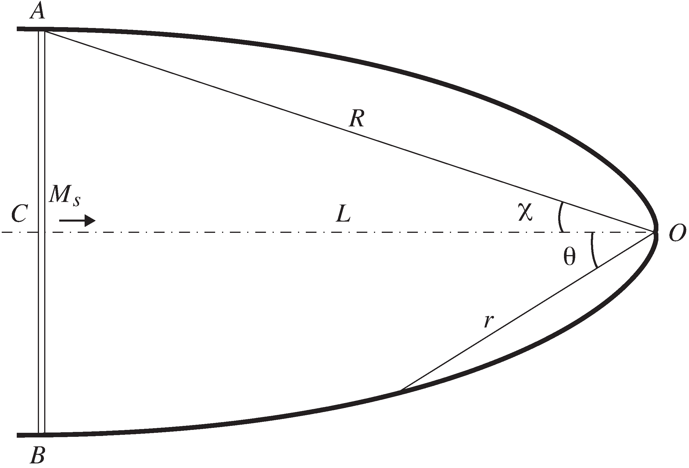
To begin with, the cases presented in [15] are repeated here using Overture so that a direct comparison of results with the new obstacle configuration is possible. First, two cases were simulated using the full Navier–Stokes equations. In the first case, the obstacles were cylinders with diameter $d=8.8$ mm placed in a non-staggered matrix (NS) based on four rows, each containing four obstacles; Figure 4. The second case is a logarithmic spiral case with square obstacles. The Reynolds number for these cases is approximately $Re=21,900$, which is calculated as $Re=\rho UL/\mu$. Here, $\rho =1.2$ kg/m${}^3$, $U=343.8$ m/s, $L=0.001$ m and dynamic viscosity $\mu =1.864\times {10}^{-5}$ kg/(ms). The Prandtl number is set to be $Pr=0.72$, and the thermal conductivity is $\kappa =\mu /Pr\approx 0.000064$. Pressure $p_1$ is defined as the initial pressure set in the low pressure part of the shock tube, $p_1=13,330$Pa, and $p_2$ is the initial high pressure behind the incident shock wave, $p_2=28,260$Pa. Then, the simulations were repeated using the inviscid Euler equations, and the results were compared.

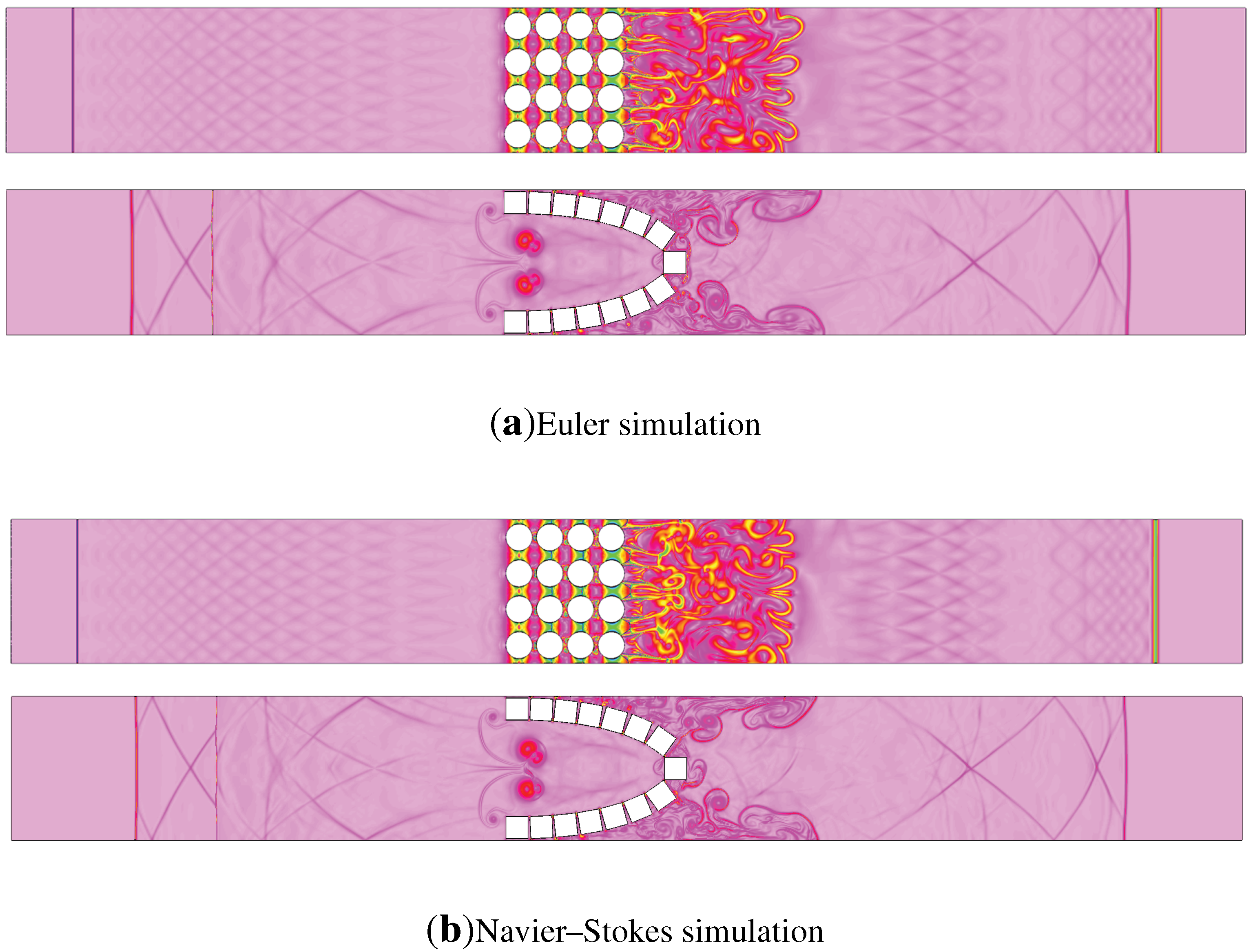
Figure 4 shows schlieren contours of the results from Euler and Navier–Stokes simulations for the two cases. The primary difference in the graphs is in the turbulent region occurring behind the matrix of obstacles. The addition of viscosity does not affect the simulation results in terms of reflected and transmitted shock locations.

Figure 4. Schlieren contour for shock wave propagation past non-staggered cylindermatrix and squares along a logarithmic spiral under (a) inviscid Euler equations and (b) full Navier–Stokes equations.

Figure 4. Schlieren contour for shock wave propagation past non-staggered cylindermatrix and squares along a logarithmic spiral under (a) inviscid Euler equations and (b) full Navier–Stokes equations.

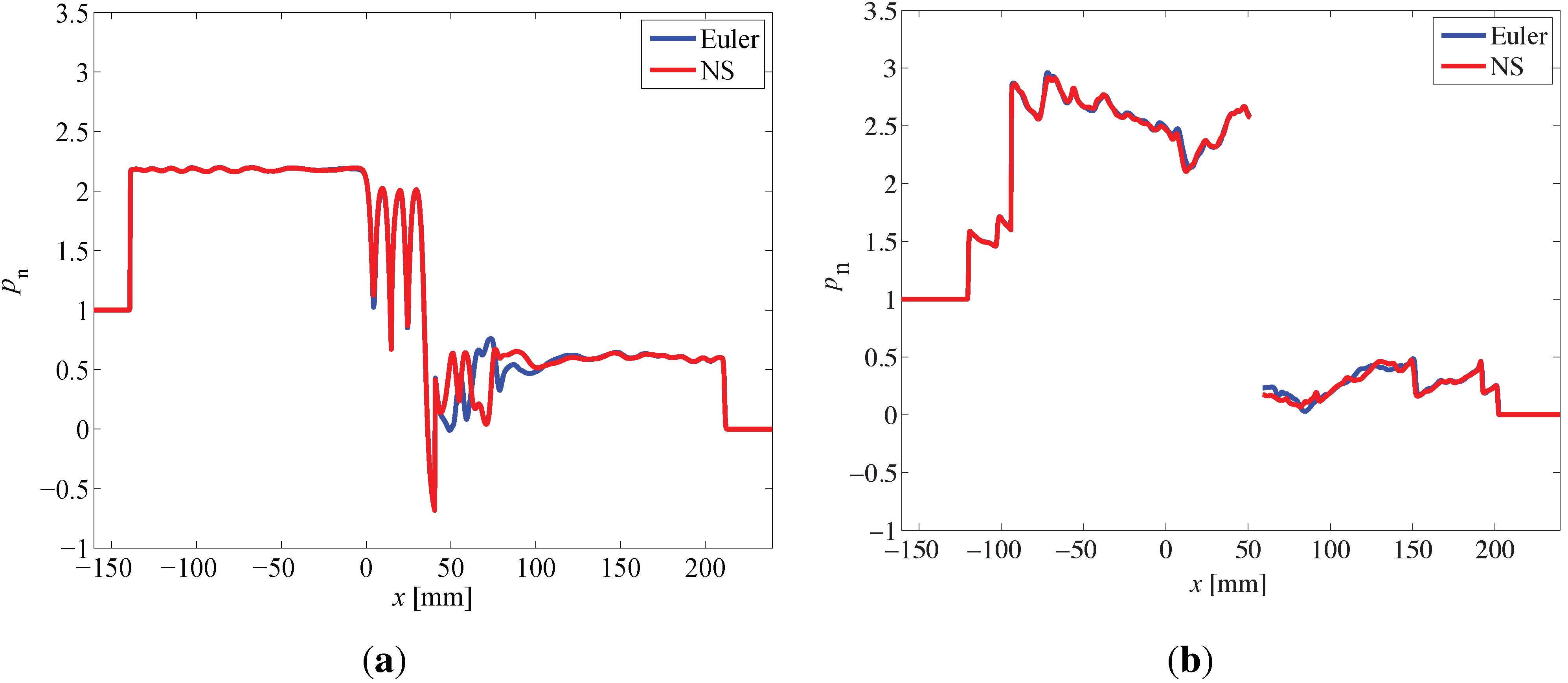
The corresponding non-dimensional pressure ($p_n$) for these two cases is plotted in Figure 5 at $t=500\mu$s. The curves in Figure 5b are discontinuous due to the obstacle placed at the centerline. The non-dimensional pressure is defined as $p_n=(p-p_1)/(p_2-p_1)$, where p is dimensional pressure measured by the probe. As shown in the figure, the reflected and transmitted shock waves are at the same location for the two simulations, and the amplitudes of the peak pressures are the same for both cases. The only difference of the two cases is the area with the turbulence right behind the obstacles. From the collected pressure data at the downstream probe for the non-staggered cylinder (NC) and logarithmic spiral square (LSS) cases (for a grid resolution $\Delta x\approx 0.24$ mm for the background grid and the smallest grid size $\Delta x\approx 60\mu$m, including AMR), the difference is only 2.6% for NC and 2.7% for LSS between time-averaged non-dimensional pressures for full Navier–Stokes and inviscid Euler simulation.

Figure 5. Dimensionless pressure, $p_n$, along the centerline for Navier–Stokes and Euler simulations at time instant $t=500$ μs for non-staggered cylinders (NC) and logarithmic spiral squares (LSS). (a) NC; (b) LSS.

Figure 5. Dimensionless pressure, $p_n$, along the centerline for Navier–Stokes and Euler simulations at time instant $t=500$ μs for non-staggered cylinders (NC) and logarithmic spiral squares (LSS). (a) NC; (b) LSS.

Moreover, to quantify the effect of viscosity, the standard deviation between the Euler and theNavier–Stokes results shown in Figure 5 was calculated. Pressure data was collected at 2000 points along the centerline of the shock tube for both cases at a time instant of $t=500$ μs. Then, the pressure difference between the two sets of simulation data for each point in space was calculated. Thus, a dataset containing pressure differences was obtained, for which every element should be close to zero. The standard deviation, ${\sigma }_p$, of this dataset was calculated using Equation (11).

$$\begin{array}{c}{\sigma }_p=\sqrt{\frac{1}{N}\sum _{i=1}^N{(d{p}_i-d{p}_{av})}^2}\end{array}$$

(11)

where N is the total number of the data points, $N=2000$, $d{p}_i$ is the pressure difference at each point between the Euler and Navier–Stokes simulations and $d{p}_{av}$ is the average pressure difference along the centerline. The standard deviation for pressure difference of the LSS case is $522$Pa along the centerline, which is only 2.5% of the initial constant inlet high pressure, $p_2=28,260$Pa. The standard deviation for pressure difference of the NC case is $1839$Pa, which is about 6.5% of the initial constant inlet high pressure. Therefore, because these differences were small and the choice of equations does not influence the shock positions, the rest of the cases were run using the Euler equations.

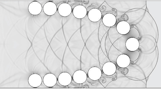
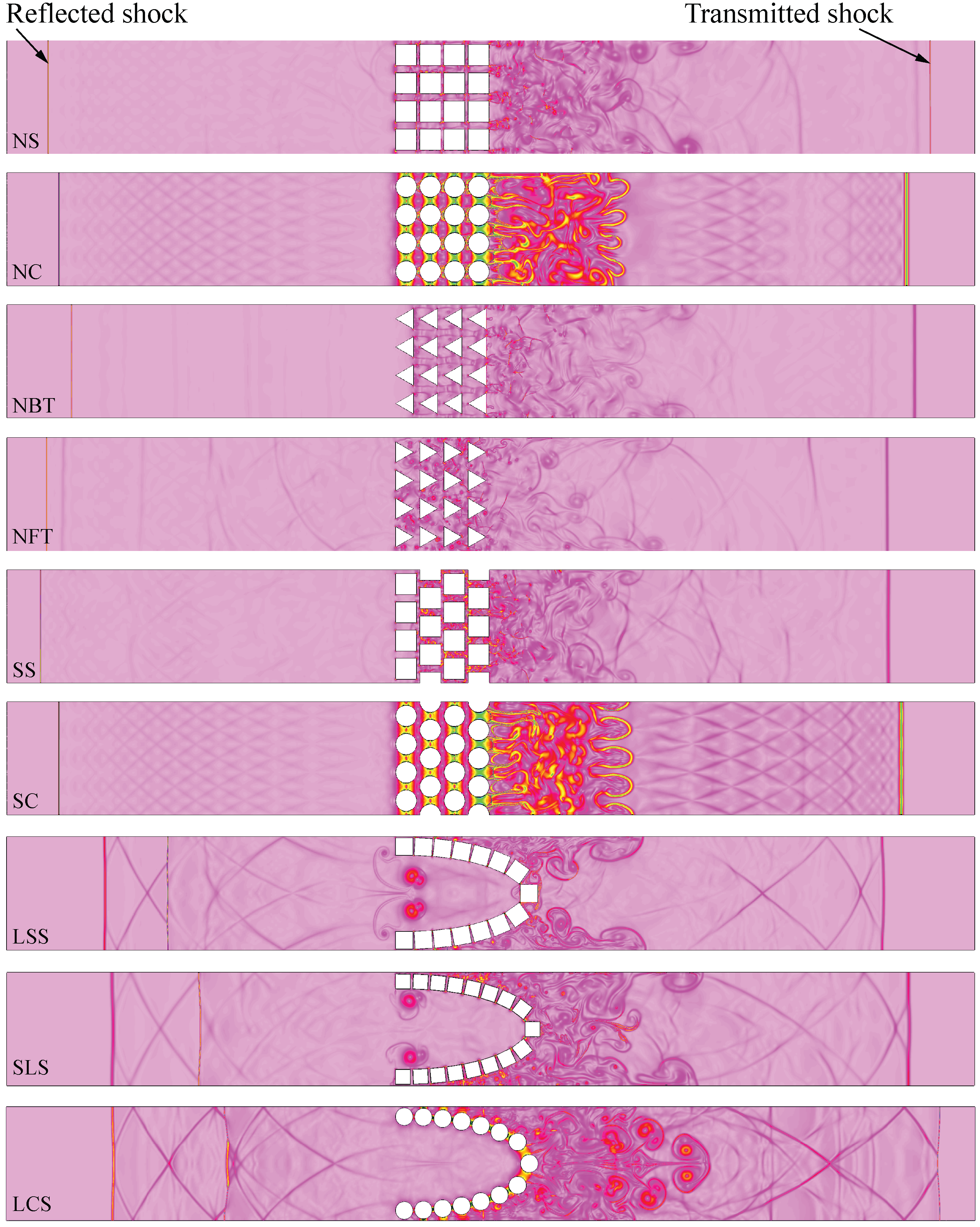
3.1. Numerical Results for Obstacle Arrays

Collection of data starts when the shock wave first impacts the leading edge of the obstacles, and the simulation then lasts for about 500 μs. Numerical schlieren plots for nine different obstacle configurations at time instant $t=500$ μs are shown in Figure 6. The first four cases, from top to bottom, are arranged in non-staggered columns (NS, NC, non-staggered forward triangle (NFT), non-staggered backward triangle (NBT)). The fifth and sixth cases (staggered square (SS) and staggered cylinder (SC)) are arranged in staggered patterns. The obstacles in the seventh, eighth and ninth cases are placed along a logarithmic spiral (LSS, SLS, logarithmic spiral cylinder (LCS)). The reflected and transmitted shocks and vortices behind the obstacles are clearly visualized in the schlieren plots. Of the first six cases, the NFT case most efficiently minimizes the transmitted shock, and NBT most efficiently reduces the reflected shock wave. The fluid velocities downstream of the obstacle arrays are smaller for staggered cases than non-staggered cases.

Figure 6. Top to bottom: NS, NC, NBT, NFT, SS, SC, LSS, SLS and LCS schlieren contours taken at $t=500$ μs after the shock first impacts the obstacle array. The locations of the incident shock wave and the reflected shock wave are marked with arrows. Note: the first six cases, from top to bottom, are reproduced from [15].

Figure 6. Top to bottom: NS, NC, NBT, NFT, SS, SC, LSS, SLS and LCS schlieren contours taken at $t=500$ μs after the shock first impacts the obstacle array. The locations of the incident shock wave and the reflected shock wave are marked with arrows. Note: the first six cases, from top to bottom, are reproduced from [15].

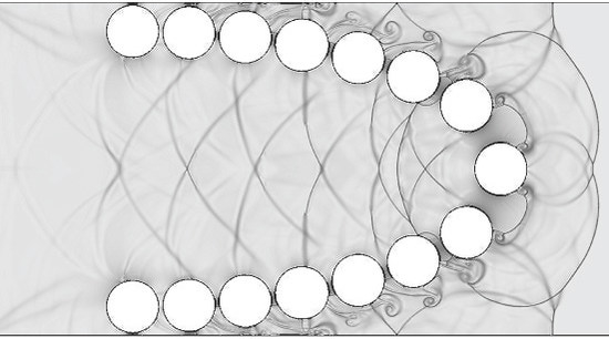
In the LSS case, not only is the transmitted shock delayed more than for the previous cases, but the reflected shock wave is also delayed. Part of the shock propagates through the barrier, while the rest is reflected. The gaps between the square obstacles change the direction of portions of the incident shock, deflecting it towards the walls of the shock tube. Therefore, some of the energy is lost through dissipation near the walls as vortices are formed. During shock wave propagation through the obstacles, part of the initial horizontal kinetic energy is converted to kinetic energy in the vertical direction, especially in regions around the slits between adjacent square obstacles. In these areas, more than 80%–90% of the kinetic energy has been directed in the vertical direction after 250 μs.

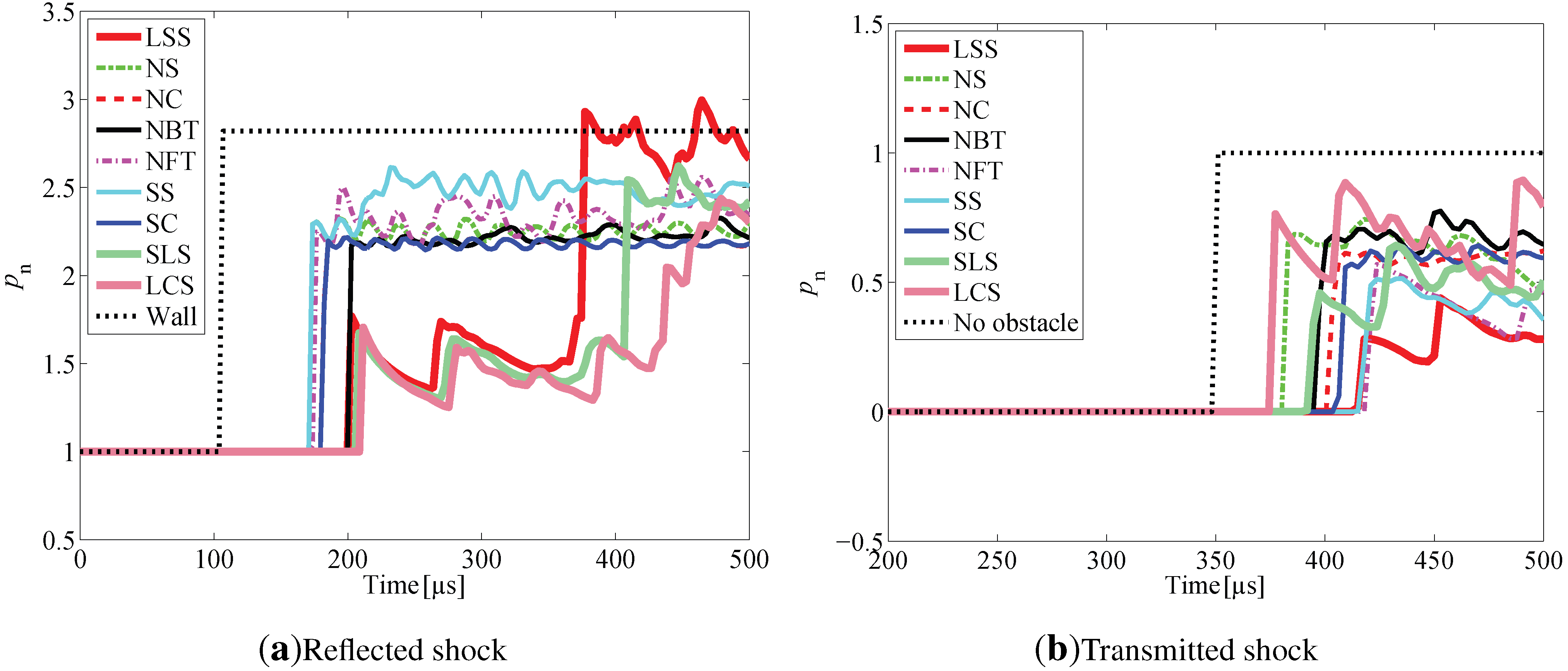
Non-dimensional pressures as functions of time recorded at both probe locations for all cases are shown in Figure 7. In addition to the cases described earlier, reflection from a solid wall located at the leading edge, $x=0$, and incident shock propagation without encountering any type of obstacles are also taken into consideration for comparison purposes. For all cases, there is a pressure jump when the shock wave initially reaches the probe. For most cases, the pressure oscillates around a particular high pressure. As seen in Figure 7b, the pressure for the LSS case is smaller than the rest of the cases. However, as seen in Figure 7a, the pressure amplitude of the reflected shock for the LSS case is lower than other cases, but for later times, the peak pressure is the highest. Note that in the LSS case shown in Figure 6, there are two reflected shocks traveling leftward. The first shock is the reflection from the leading edge of the obstacles, while the second shock following behind the first reflected shock is the reflection from the deep end of the logarithmic spiral curve. For other matrix cases, only one reflected shock is generated. Comparing with other cases, the first reflected shock is weaker than that in other cases, because the pressure amplitude of the first reflected shock is lower than other cases. The pressure jump across the second shock is higher, so the second reflected shock is stronger than the first.

Figure 7. Plot of dimensionless pressure, $p_n$, at (a) upstream probe $(x,y)=(-50,0)$ and (b) downstream probe $(x,y)=(169.4,0)$, as functions of time for all cases.

Figure 7. Plot of dimensionless pressure, $p_n$, at (a) upstream probe $(x,y)=(-50,0)$ and (b) downstream probe $(x,y)=(169.4,0)$, as functions of time for all cases.

The time-averaged overpressure after the shock reaches the probes and the time when the shock wave arrives at the probes are two indicators that measure the effectiveness of the obstacle barriers. The time-averaged overpressure is defined as $\overline{\mathcal{P}}=(\overline{p}-p_1)/(p_2-p_1)$. The time-averaged pressure, $\overline{p}$, is defined as $\overline{p}=\frac{1}{\Delta \mathcal{T}}{\int }_{t_0}^{t_f}p\mathrm{d}t$, $\Delta \mathcal{T}=t_f-t_0$, where $t_f$ and $t_0$ are the final and start time when pressure data are collected. Using subscript r to denote the overpressure for the reflected shock and subscript t to denote the overpressure for the transmitted shock, the time-averaged overpressure data, ${\overline{\mathcal{P}}}_r$ and ${\overline{\mathcal{P}}}_t$, collected at the probes from time $t_0$ to $t_f$ are presented in Table 2, along with the times, $t_{pr}$ and $t_{pt}$, when the shock reaches the probes. Larger $t_{pr}$ and $t_{pt}$ and smaller ${\overline{\mathcal{P}}}_r$ and ${\overline{\mathcal{P}}}_t$ mean that the obstacles more efficiently attenuate the incident shock wave. Results show that the LSS case produces the smallest time-averaged pressure in the region downstream of the obstacle area, for all cases, and in the upstream region, it is smaller than the matrix arrangements, but larger than the SLS and LCS cases.

Table 2. Comparison of time-averaged overpressure ${\overline{\mathcal{P}}}_r$, ${\overline{\mathcal{P}}}_t$, shock arrival time at the upstream probe, $t_{pr}$, and downstream probe, $t_{pt}$, and the difference $E_{\overline{\mathcal{P}}}$. ${}^{★}$ Results reported in [15].

Case	${\overline{\mathcal{P}}}_r$	${\overline{\mathcal{P}}}_t$	$t_{\mathrm{pr}}$ (μs)	$t_{\mathrm{pt}}$ (μs)	$E_{\overline{\mathcal{P}}}$ (%)
NS	2.25	0.61 (0.58 ${}^{★}$)	174	377	5.2
NC	2.18	0.54 (0.56 ${}^{★}$)	182	395	−3.6
NBT	2.22	0.62 (0.55 ${}^{★}$)	203	389	12.7
NFT	2.33	0.38 (0.37 ${}^{★}$)	174	412	2.7
SS	2.47	0.38 (0.24 ${}^{★}$)	174	406	58.3
SC	2.18	0.54 (0.55 ${}^{★}$)	182	398	−1.8
LSS	2.06	0.27 (−)	203	409	–
SLS	1.79	0.43 (−)	209	383	–
LCS	1.62	0.66 (−)	211	374	–

Table 2. Comparison of time-averaged overpressure ${\overline{\mathcal{P}}}_r$, ${\overline{\mathcal{P}}}_t$, shock arrival time at the upstream probe, $t_{pr}$, and downstream probe, $t_{pt}$, and the difference $E_{\overline{\mathcal{P}}}$. ${}^{★}$ Results reported in [15].

Case	${\overline{\mathcal{P}}}_r$	${\overline{\mathcal{P}}}_t$	$t_{\mathrm{pr}}$ (μs)	$t_{\mathrm{pt}}$ (μs)	$E_{\overline{\mathcal{P}}}$ (%)
NS	2.25	0.61 (0.58 ${}^{★}$)	174	377	5.2
NC	2.18	0.54 (0.56 ${}^{★}$)	182	395	−3.6
NBT	2.22	0.62 (0.55 ${}^{★}$)	203	389	12.7
NFT	2.33	0.38 (0.37 ${}^{★}$)	174	412	2.7
SS	2.47	0.38 (0.24 ${}^{★}$)	174	406	58.3
SC	2.18	0.54 (0.55 ${}^{★}$)	182	398	−1.8
LSS	2.06	0.27 (−)	203	409	–
SLS	1.79	0.43 (−)	209	383	–
LCS	1.62	0.66 (−)	211	374	–

A direct comparison between the pressure values reported in [15] (all obtained from the full Navier–Stokes equations) and the ones presented here (using the inviscid Euler equations) shows somewhat different results, with comparable results for NS, NC, NFT and SC cases (<$6\%$ difference), somewhat comparable to the NBT case (<$13\%$ difference), but a large discrepancy for the SS case (<$60\%$ difference); see Table 2. One likely reason that the SS cases are different is the way the obstacles are represented. Here, the squares have slightly rounded corners, and this will influence the flow around them. A comparison among the logarithmic spiral cases shows that the transmitted shock for both the LCS and the SLS case reach the probe earlier than the LSS case. This is due to a combination of obstacle shape and gap size between obstacles; more details on effective flow area are in Section 3.3.

Then, the impulse for both reflected and transmitted shocks is computed for three different time intervals; see Table 3. The impulses are calculated from the time when the reflected shock reaches the probe, and only the pressure that is higher than the initial pressure before the shock arrives contributes to the impulse. The reflected shocks reach the probe relatively early in the simulation, so the impulses were calculated for 100-, 200- and 300-μs time intervals. The transmitted shocks reach the probe at a later time, so the impulses were calculated for shorter time spans of 30, 60 and 90 μs. For the transmitted shock, the LSS case results in the lowest impulse, and for the reflected shock, the LSS case is lower than any of the matrix-arranged obstacles, but higher than the other two logarithmic spiral shapes.

Table 3. Impulse, I, recorded by the upstream (reflected shock) and downstream (transmitted shock) probes for three time intervals. Units in Pa·s.

Case	Reflected Shock				Transmitted shock
	$I_{100}$	$I_{200}$	$I_{300}$		$I_{30}$	$I_{60}$	$I_{90}$
NS	1.87	3.74	5.61		0.24	0.55	1.24
NC	1.75	3.51	5.27		0.18	0.45	1.11
NBT	1.77	3.61	5.46		0.20	0.50	1.22
NFT	1.88	3.88	5.94		0.16	0.35	0.92
SS	2.12	4.36	6.55		0.13	0.32	0.91
SC	1.75	3.51	5.27		0.23	0.50	1.17
LSS	0.84	2.13	4.75		0.08	0.23	0.76
SLS	0.72	1.44	3.60		0.11	0.32	0.96
LCS	0.67	1.31	2.88		0.25	0.60	1.29

Table 3. Impulse, I, recorded by the upstream (reflected shock) and downstream (transmitted shock) probes for three time intervals. Units in Pa·s.

Case	Reflected Shock				Transmitted shock
	$I_{100}$	$I_{200}$	$I_{300}$		$I_{30}$	$I_{60}$	$I_{90}$
NS	1.87	3.74	5.61		0.24	0.55	1.24
NC	1.75	3.51	5.27		0.18	0.45	1.11
NBT	1.77	3.61	5.46		0.20	0.50	1.22
NFT	1.88	3.88	5.94		0.16	0.35	0.92
SS	2.12	4.36	6.55		0.13	0.32	0.91
SC	1.75	3.51	5.27		0.23	0.50	1.17
LSS	0.84	2.13	4.75		0.08	0.23	0.76
SLS	0.72	1.44	3.60		0.11	0.32	0.96
LCS	0.67	1.31	2.88		0.25	0.60	1.29

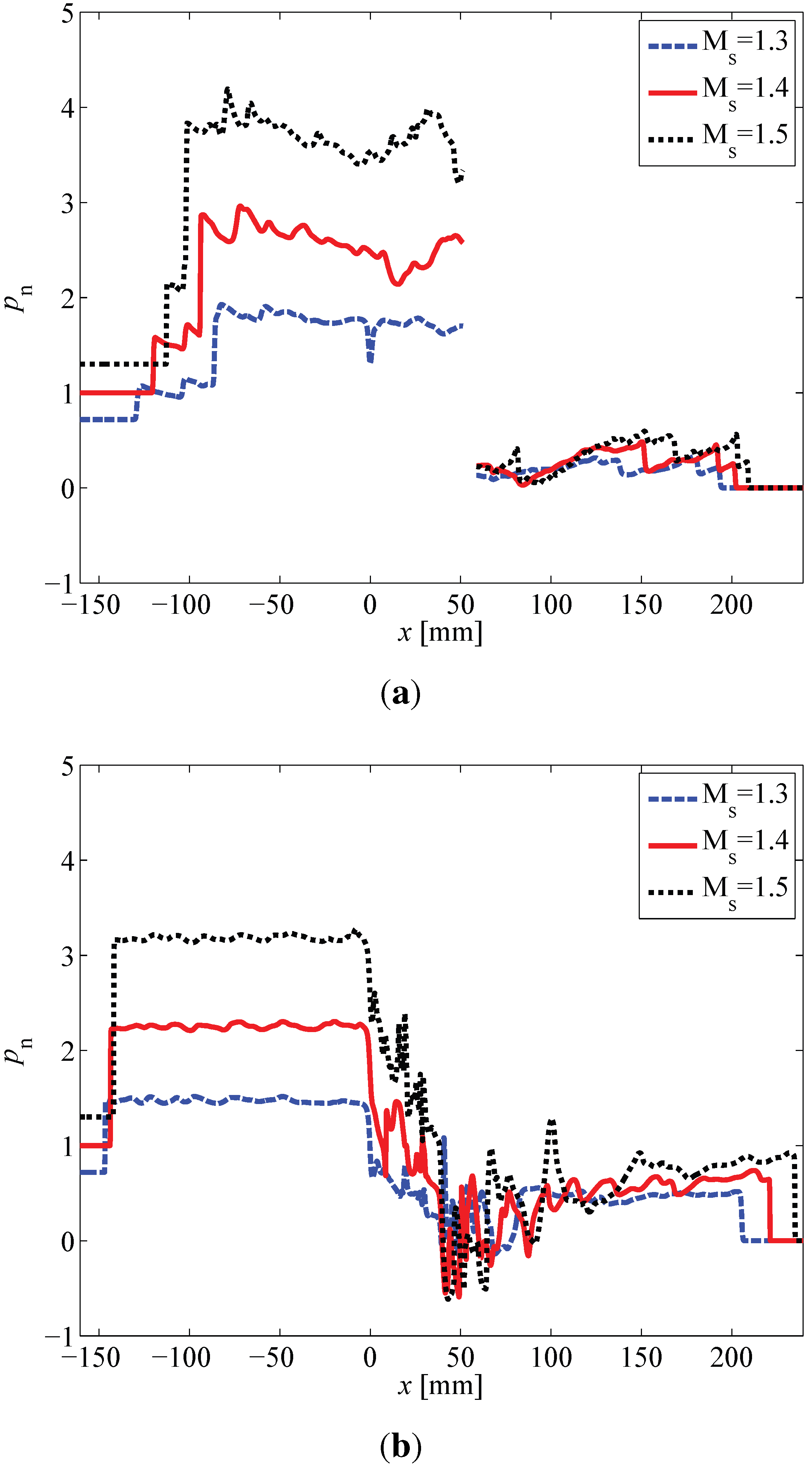
3.2. Effects of Incident Shock Mach Number

Because the logarithmic spiral shape used here is designed for a specific incident shock Mach number, $M_s=1.4$, two additional cases, $M_s=1.3$ and $M_s=1.5$, were simulated to understand how well this particular shape works for off-design Mach numbers. Figure 8 shows the pressure distribution along the centerline for $M_s$ = 1.3, 1.4 and 1.5 for the LSS and NS cases at $t=500$ μs. The discontinuity in Figure 8a is due to the square obstacle placed at the centerline at the tip of the spiral. It can be seen that for a higher incoming Mach number, the stronger the transmitted and reflected shocks are, which is due to more energy contained in the shock wave. Especially, the pressure behind the reflected shocks increases when $M_s$ is increased from 1.3 to 1.5.

To compare the degree of shock attenuation for the reflected and transmitted shocks of the LSS and NS cases, we defined the pressure ratio of the pressure behind the shock and the initial high pressure in Table 4. Results show that for both the LSS and NS cases, the pressure ratio for $M_s=1.4$ is smaller than that for $M_s=1.3$, which means that the current logarithmic spiral shape is more effective for $M_s=1.4$ than $M_s=1.3$ to mitigate the transmitted shock and similarly for the NS case. However, for $M_s=1.5$ in the LSS case, this pressure ratio is even lower than the $M_s=1.4$ case, which means that the transmitted shock is more attenuated for higher shock Mach numbers. However, for the NS case at $M_s=1.5$, the pressure ratio is higher than the ratio for $M_s=1.4$. Comparing upstream pressure ratios for the NS with the LSS case, it is found that the pressure ratios behind the reflected shock for the NS cases are all lower than the LSS cases, with 16% lower on average.

Figure 8. Dimensionless pressure, $p_n$, along the centerline of (a) LSS and (b) NS for $M_s=1.3,1.4$ and $1.5$ at time instant $t=500$ μs.

Figure 8. Dimensionless pressure, $p_n$, along the centerline of (a) LSS and (b) NS for $M_s=1.3,1.4$ and $1.5$ at time instant $t=500$ μs.

Table 4. The ratio of the peak pressure measured behind the transmitted and reflected shocks along the centerline of the shock tube at time $t=500$ μs to the initial high pressure behind the incident shock, $q_{pt}$ and $q_{pr}$, where the subscript t denotes transmitted shock and r denotes reflected shock.

Case	LSS				NS
	$M_s=1.3$	$M_s=1.4$	$M_s=1.5$		$M_s=1.3$	$M_s=1.4$	$M_s=1.5$
$q_{pt}$	0.757	0.728	0.678		1.23	0.861	0.985
$q_{pr}$	1.75	2.04	2.32		1.50	1.69	1.90

Table 4. The ratio of the peak pressure measured behind the transmitted and reflected shocks along the centerline of the shock tube at time $t=500$ μs to the initial high pressure behind the incident shock, $q_{pt}$ and $q_{pr}$, where the subscript t denotes transmitted shock and r denotes reflected shock.

Case	LSS				NS
	$M_s=1.3$	$M_s=1.4$	$M_s=1.5$		$M_s=1.3$	$M_s=1.4$	$M_s=1.5$
$q_{pt}$	0.757	0.728	0.678		1.23	0.861	0.985
$q_{pr}$	1.75	2.04	2.32		1.50	1.69	1.90

Doing the same comparison for the reflected shock yields a different result. As shown in Table 4, the reflected shock has been most effectively attenuated for the lower Mach number cases and least for the higher Mach number case. Comparing NS with LSS regarding the pressure ratios at the downstream position shows that the pressure ratios behind the transmitted shock for the LSS cases are all lower than the NS cases, about 28% lower on average. To sum up, this logarithmic spiral shape, initially designed for $M_s=1.4$, has a higher ability of decreasing the pressure of transmitted shocks for incident Mach numbers that are larger or equal to the design Mach number, than Mach numbers that are lower than the design Mach number. On the other hand, this shape reduces the pressure of the reflected shock more when the incident Mach number is less than or equal to the design Mach number compared to the higher Mach number cases.

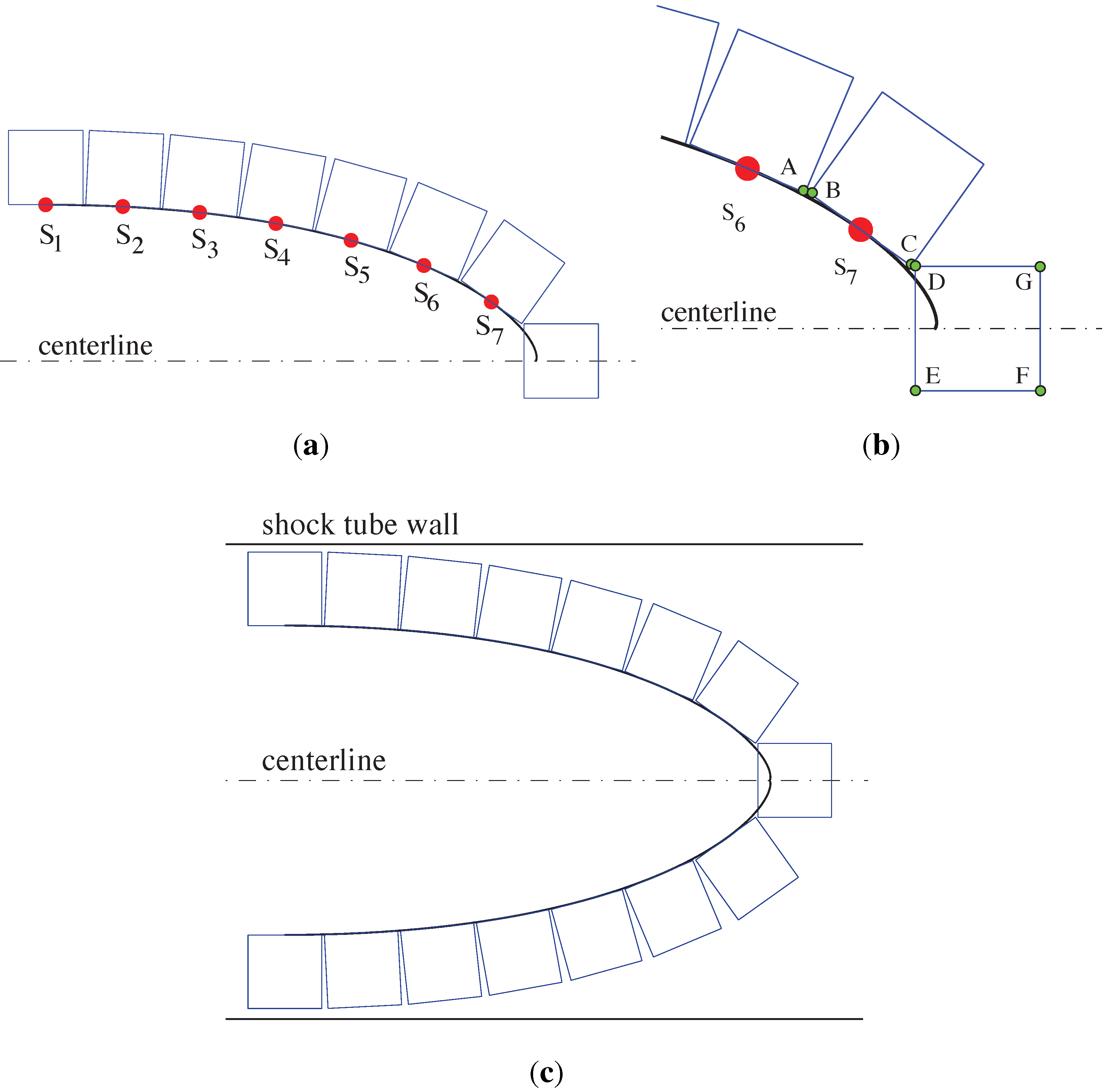
3.3. Effective Flow Area and Sensitivity of Obstacle Size

To be able to compare the result from one case to another, one way is to define an effective flow area. The effective flow area with regard to the gaps along the columns in [15] is defined as follows,

$$\begin{array}{c}{ϵ}_1=1-\sum _{i=1}^{N_c}(D_i/H)\end{array}$$

(12)

where $N_c$ is the number of obstacles in a column, $D_i$ is the diameter of the i-th obstacle and H is the height of the shock tube. For the logarithmic spiral cases, the obstacles are not placed in subsequent columns, so the effective flow area is calculated with the following formula,

$$\begin{array}{c}{ϵ}_2=\sum _{i=1}^{N_s}{S}_{yi}/H\end{array}$$

(13)

where $N_s$ is the number of gaps and $S_{yi}$ is the gap size projection in the y-direction perpendicular to the shock propagation direction). Table 5 summarizes the effective flow area for all cases. If, instead, the gap projection area in the x-direction is used,

$$\begin{array}{c}{ϵ}_3=\sum _{i=1}^{N_s}{S}_{xi}/H\end{array}$$

(14)

where $S_{xi}$ is the gap size projection in the x-direction (shock propagation direction).

By comparing the previous results from Table 2 and Table 5, with an ${ϵ}_2$ for SLS $295.6\%$ larger than that for the LSS case and with an ${ϵ}_3$$187.5\%$ larger than that for the LSS case, the overpressure for the transmitted shock, ${\overline{\mathcal{P}}}_t$, has a $59\%$ increase, while the overpressure for the reflected shock, ${\overline{\mathcal{P}}}_r$, has a $13\%$ decrease. Thus, the overpressure downstream is increasing rapidly, and overpressure upstream is decreasing relatively slow as ${ϵ}_2$ and ${ϵ}_3$ increase for the logarithmic spiral cases. The geometric pattern of placing the square obstacles is similar in both the SLS and LSS case. However, the effective flow area is different. It is likely that the transmitted shock travels faster in the SLS case than in LSS case due to the increase of the gap size between the obstacles.

Table 5. The effective flow area. For matrix arrangements, case NC–SS, Equation (12) is used to calculate ${ϵ}_1$, and for logarithmic spiral cases, LSS–SLS, Equation (13) is used to calculate ${ϵ}_2$.

Case	${ϵ}_1$ or ${ϵ}_2$	${ϵ}_3$
NC	0.25	–
NS	0.25	–
SC	0.25	–
NBT	0.25	–
NFT	0.25	–
SC	0.25	–
SS	0.25	–
LSS	0.0091	0.080
LCS	0.14	0.21
SLS	0.036	0.23

Table 5. The effective flow area. For matrix arrangements, case NC–SS, Equation (12) is used to calculate ${ϵ}_1$, and for logarithmic spiral cases, LSS–SLS, Equation (13) is used to calculate ${ϵ}_2$.

Case	${ϵ}_1$ or ${ϵ}_2$	${ϵ}_3$
NC	0.25	–
NS	0.25	–
SC	0.25	–
NBT	0.25	–
NFT	0.25	–
SC	0.25	–
SS	0.25	–
LSS	0.0091	0.080
LCS	0.14	0.21
SLS	0.036	0.23

4. Conclusions

In this paper, the behavior of a planar shock wave propagating in a shock tube, passing through obstacles of various geometries, placed in non-staggered, staggered or logarithmic spiral patterns is simulated. The results presented here show that a logarithmic spiral can be used to attenuate a planar incident shock wave. The results indicate that the logarithmic spiral decreases the pressure and delays the shock velocity downstream of the obstacles for certain ranges of Mach numbers. Additionally, the reflected shock is effectively delayed, but the pressure ratio remains relatively high. Therefore, when the reflected shock is fully developed, much later than the time span shown in the presented simulations, it may catch up with the reflected shocks in the other simulated cases. In reality, it might still be a viable solution to use a logarithmic spiral compared to matrix arrangements, since viscosity will act on the flow, and the longer the shock wave is delayed, the more it will dissipate.

When comparing different logarithmic spiral cases, SLS and LSS, the strength of the transmitted and reflected shock is determined both by the size of the gaps and the size of the obstacles. The effect of the gap size is particularly obvious for the logarithmic spiral cases LSS and LCS. To explore how a logarithmic spiral designed for one particular shock Mach number mitigates shock waves with off-design Mach numbers, two cases were simulated. By comparing the results of a higher ($M_s=1.5$) and a lower Mach number ($M_s=1.3$) case than the intended design Mach number ($M_s=1.4$), two trends are confirmed: (1) the pressure ratio of the transmitted shock to that of the high pressure behind the shock, $p_2$, is reduced to a greater extent for higher Mach numbers; and (2) the pressure ratio of the reflected shock to that of the initial high pressure is reduced for lower Mach numbers. Therefore, as expected, the attenuation of the LSS also depends on the Mach number of the incident shock wave.

Future directions of this research will be to investigate the same scenario using an obstacle material that can help to further attenuate the shock wave. In this paper, only rigid obstacles were considered, which results in a significant shock attenuation. By choosing the obstacle material wisely, larger shock attenuation should be possible.

References

1. Perry, R.W.; Kantrowitz, A. The production and stability of converging shock waves. J. Appl. Phys. 1951, 22, 878–886. [Google Scholar] [CrossRef]
2. Balasubramanian, K.; Eliasson, V. Numerical investigations of the porosity effect on the shock focusing process. Shock Waves 2013, 23, 583–594. [Google Scholar] [CrossRef]
3. Eliasson, V.; Apazidis, N.; Tillmark, N. Controlling the form of strong converging shocks by means of disturbances. Shock Waves 2007, 17, 29–42. [Google Scholar] [CrossRef]
4. Kjellander, M.; Tillmark, N.; Apazidis, N. Experimental determination of self-similarity constant for converging cylindrical shocks. Phys. Fluids 2011, 23, 116103. [Google Scholar] [CrossRef]
5. Takayama, K.; Kleine, H.; Grönig, H. An experimental investigation of the stability of converging cylindrical shock waves in air. Exp. Fluids 1987, 5, 315–322. [Google Scholar] [CrossRef]
6. Takayama, K.; Onodera, O.; Hoshizawa, Y. Experiments on the stability of converging cylindrical shock waves. Theor. Appl. Mech. 1984, 32, 117–127. [Google Scholar]
7. Watanabe, M.; Onodera, O.; Takayama, K. Shock wave focusing in a vertical annular shock tube. In Shock Waves @ Marseille IV; Springer: Berlin, Germany, 1995; pp. 99–104. [Google Scholar]
8. Dosanjh, D.S. Interaction of Grids with Traveling Shock Waves; NACA Technical Note 3680; Johns Hopkins University: Washington, DC, USA, 1956. [Google Scholar]
9. Shi, H.; Yamamura, K. The interaction between shock waves and solid spheres arrays in a shock tube. Acta Mech. Sin. 2004, 20, 219–227. [Google Scholar]
10. Britan, A.; Karpov, A.V.; Vasilev, E.I.; Igra, O.; Ben-Dor, G.; Shapiro, E. Experimental and Numerical Study of Shock Wave Interaction with Perforated Plates. J. Fluids Eng. 2004, 126, 399. [Google Scholar] [CrossRef]
11. Britan, A.; Igra, O.; Ben-Dor, G.; Shapiro, H. Shock wave attenuation by grids and orifice plates. Shock Waves 2006, 16, 1–15. [Google Scholar] [CrossRef]
12. Naiman, H.; Knight, D. The effect of porosity on shock interaction with a rigid, porous barrier. Shock Waves 2007, 16, 321–337. [Google Scholar] [CrossRef]
13. Seeraj, S.; Skews, B.W. Dual-element directional shock wave attenuators. Exp. Therm. Fluid Sci. 2009, 33, 503–516. [Google Scholar] [CrossRef]
14. Berger, S.; Sadot, O.; Ben-Dor, G. Experimental investigation on the shock-wave load attenuation by geometrical means. Shock Waves 2009, 20, 29–40. [Google Scholar] [CrossRef]
15. Chaudhuri, A.; Hadjadj, A.; Sadot, O.; Ben-Dor, G. Numerical study of shock-wave mitigation through matrices of solid obstacles. Shock Waves 2013, 23, 91–101. [Google Scholar] [CrossRef]
16. Chaudhuri, A.; Hadjadj, A.; Sadot, O.; Glazer, E. Computational study of shock-wave interaction with solid obstacles using immersed boundary methods. Int. J. Numer. Meth. Eng. 2012, 89, 975–990. [Google Scholar] [CrossRef]
17. Henshaw, W.D.; Schwendeman, D.W. An adaptive numerical scheme for high-speed reactive flow on overlapping grids. J. Comput. Phys. 2003, 191, 420–447. [Google Scholar] [CrossRef]
18. Henshaw, W.D.; Schwendeman, D.W. Moving overlapping grids with adaptive mesh refinement for high-speed reactive and non-reactive flow. J. Comput. Phys. 2006, 216, 744–779. [Google Scholar] [CrossRef]
19. Inoue, O.; Takahashi, N.; Takayama, K. Shock wave focusing in a log-spiral duct. AIAA J. 1993, 31, 1150–1152. [Google Scholar] [CrossRef]
20. Inoue, O.; Imuta, S.; Milton, B.; Takayama, K. Computational study of shock wave focusing in a log-spiral duct. Shock Waves 1995, 5, 183–188. [Google Scholar] [CrossRef]
21. Wang, C.; Eliasson, V. Shock wave focusing in water inside convergent structures. Int. J. Multiphys. 2012, 6, 267–282. [Google Scholar] [CrossRef]
22. Wang, C.; Qiu, S.; Eliasson, V. Quantitative pressure measurement of shock waves in water using a schlieren-based visualization technique. Exp. Techn. 2013. [Google Scholar] [CrossRef]
23. Milton, B.; Archer, R. Generation of implosions by area change in a shock tube. AIAA J. 1969, 7, 779–780. [Google Scholar]
24. Whitham, G. Linear and Nonlinear Waves; Wiley-Interscience: New York, NY, USA, 1974. [Google Scholar]