Deconstructing Global Temperature Anomalies: An Hypothesis

540 First Avenue West, Qualicum Beach, BC V9K 1J8, Canada
Climate 2017, 5(4), 83; https://doi.org/10.3390/cli5040083
Submission received: 23 July 2017
/
Revised: 27 October 2017
/
Accepted: 31 October 2017
/
Published: 6 November 2017
Abstract
:This paper evaluates contributions to global temperature anomalies from greenhouse gas concentrations and from a source of natural variability. There is no accepted causation for the apparent interrelationships between multidecadal oscillations and regime changes in atmospheric circulation, upwelling, and the slowdowns in global surface temperatures associated with a ~60-year oscillation. Exogenous tidal forcing is hypothesized as a major causal agent for these elements, with orthogonal components in tidal forcing generating zonal and meridional regime-dependent processes in the climate system. Climate oscillations are simulated at quasi-biennial to multidecadal timescales by tidal periodicities determined by close approaches of new or full moon to the earth. Subtracting a tidal analog of the ~60-year oscillation from global mean surface temperatures reveals an exponential component comparable with greenhouse gas emission scenarios, and which is responsible for almost 90% or contemporary global temperature increases. Residual subdecadal temperature anomalies correlate with the subdecadal variability of evolved carbon dioxide (CO2), ENSO activity and tidal components, and indicate a causal sequence from tidal forcing to greenhouse gas (GHG) release to temperature increase. Tidal periodicities can all be expressed in terms of four fundamental frequencies. Because of the potential importance of this formulation, tests are urged using general circulation models.
1. Introduction
1.1. Background
Global temperatures and sea surface temperatures (SSTs) vary over ranges that include multidecadal to quasi-biennial. A current controversy concerns the presence and nature of decadal-scale slowdowns in global temperature anomalies, particularly the recent slowdown from about 1998 to the present [1,2]. This slowdown “has provided the scientific community with a valuable opportunity to advance understanding of internal variability and external forcing…” [3]. This paper will suggest a unifying and parsimonious physical (tidal) hypothesis to drive ocean/atmosphere variability and simulate the temporal variability of global temperature anomalies on timescales ranging from multidecadal to quasi-biennial. It is hoped that documenting the hypothesis would enable subsequent comparisons with other treatments.
Global temperature and its slowdowns have temporal patterns shared in other fields, for example the following: The Atmospheric Circulation Index (ACI) is a measure of winter wind-flow regimes from the Atlantic to West Siberia. Based on earlier work, Klyashtorin [4] classified the state of the ACI at a chosen time in terms of the accumulated difference between its zonal and meridional properties (herein referred to as Z-M). Using this formulation, the ACI exhibits a ~60-year oscillation, and regime change is signaled by a reversal in the accumulated ACI curve at a maximum or minimum. The temporal variation of detrended global temperature (and length of day, LOD) curves resemble the ACI Z-M parameter [4], although with differences of a few years in lead or lag times. The LOD varies over decades by milliseconds and is strongly correlated [5] with atmospheric angular momentum (AAM). In zonal wind regimes, the LOD increases when the earth’s rotation is slowed by a change in the earth’s mass distribution and an exchange of angular momentum between the earth’s surface and its atmosphere [6], a process promoted by precipitation or by evaporation over the oceans [7].
Dickey et al. [8] noted the common decadal variability of the LOD, and the angular momentum of the earth’s core and surface air temperatures, and found significant correlations with LOD leading model-corrected temperatures by eight years. They concluded that either oscillations in the core’s magnetic field modulated atmospheric factors, or that some other indirect effect of another fundamental process affected climate, or that there was another process that affects both.
In this journal, Oviatt et al. [9] reviewed some of these decadal patterns, drawing attention to zonal and meridional regimes that affect global temperatures, and described the effects on temperature of ocean upwelling. Global temperatures rise during zonal ACI regimes, and “pause” during meridional regimes. Following discussions at a recent workshop on decadal variability [10], the word “slowdown” will be used herein instead of the words “pause” or “hiatus” that have often been used to describe the arrested temperature rises in meridional regimes.
Oviatt et al. [9] listed three hypotheses to explain decadal shifts: (1) atmospheric–ocean interaction dynamics; (2) the rate of Atlantic meridional overturning circulation (AMOC); and (3) a statistical combination of climate indices and Arctic sea ice variability. They concluded there was no accepted causation to explain the decadal changes.
The first hypothesis includes the suggestion that the hiatus is associated with the negative phase of the Interdecadal Pacific Oscillation (IPO), and the accompanying cooling and strong easterly winds over the equatorial Pacific. The second hypothesis includes the idea that the warming hiatus is a result of large heat uptake by the deep ocean. From large ensemble simulations, Liu et al. [11] showed that, in hiatus decades, the Indian Ocean shows anomalous warming and accelerated ocean heat content increase below 50 m. This is associated with a La Niña-like climate shift and enhanced heat transport of the Indonesian Throughflow, and the warming occurs concurrently with Pacific cooling. Meridional overturning and wind-driven decadal variability in ocean basins were possible proximate causes. For further discussion of ocean heat uptake and global temperatures, see Whitmarsh et al. [12].
Several authors have noted the apparent relationship between the successive rises and pauses in global temperatures on the one hand and the temperatures and phases in Pacific-basin oscillations on the other (e.g., [1,2,13]). However, just ten of 262 model simulations with the Coupled Model Intercomparison Project Phase 5 (CMIP5) produced the early-2000s slowdown in global surface temperature rise from the decadal modulation associated with an IPO negative phase [14]).
Such empirical or computer-modeled relationships beg the question: What is the ultimate driver for ocean and climate variability? The seemingly close relationships between such oceanic, geophysical and climatic parameters may derive either from internally-generated and teleconnected terrestrial endogenous processes or through an external forcing mechanism. The possible sources of influences external to the climate system have generally focused on aerosols, volcanoes and solar irradiance, but such natural sources of variability seem to be inadequately represented in models; see for instance Trenberth [1] and Santer et al. [3].
This paper presents the hypothesis that exogenous tidal forcing from the sun and moon is a major cause of climate variability. The tidal hypothesis leads to the following propositions:
- (1)
- tidal forces from the sun and moon vary predictably;
- (2)
- these external tidal forces exist in alternately dominating meridional (approximately north–south) and zonal west–east) directions;
- (3)
- these tidal forces provide an exogenous driver of global ocean and atmospheric variability, on timescales from subdecadal to multidecadal, in a manner to some degree deterministic, predictable and testable; and
- (4)
- this exogenous forcing engenders decadal-scale slowdowns in global mean surface temperatures.
Relationships between tidal forces and climate variability may useful in long-term risk assessment for natural resource management, including fisheries applications described by Klyashtorin [4] and Oviatt et al. [9]. However, here, the hypothesis will be related only oscillations present in global mean surface temperatures and in some major climate systems on timescales from quasi-biennial to multidecadal.
1.2. The Tidal Hypothesis
The understanding of tidal effects from the sun and moon has progressed as a result of seminal studies [15,16,17], in the course of which the parameterization has become complex as more spectral components and terms have been added to the tidal potential; see for instance Kantha and Clayson [18].
Doodson [15] derived six fundamental astronomical frequencies governing the tides, with corresponding periods covering the range from a lunar day to almost 21,000 years. The three that seem most likely candidates to assist in explaining annual-to-multidecadal climate processes had periods of 1, 8.847 and 18.613 years, corresponding to intervals involving the sun’s mean longitude, the longitude of the moon’s perigee and the longitude of the moon’s ascending node. Doodson expanded the number of tidal frequencies f by adding or subtracting these frequencies or their harmonics, such as with f1 + 2f2 − f3 and so on. Adding and subtracting two frequencies (reciprocals of periods) generates two more frequencies. This process of frequency combination (sometimes called frequency demultiplication, e.g., [19]) has been invoked (for example) by Keeling and Whorf [20] and by two studies of the quasi-biennial oscillation to be described later. Such frequency combinations are a common feature of systems with interacting oscillators, as with intermodulation in electrical systems and vibration-rotation bands in spectroscopy. Treloar [21] chose an approach that has become accessible in recent decades. As the tidal potential depends on the distances and directions of the sun and moon in relation to the earth, the latter parameters can be computed from astronomical polynomial algorithms [22], which are reasonably accurate over several centuries. Using this source, and with a simple physical model reflecting the combined mass/distance3 contributions from sun and moon, three-dimensional tidal forces varying over time were partitioned into components parallel and perpendicular to the plane of the moon’s orbit, approximately equivalent to zonal and meridional (or east–west and north–south) earth-based directions respectively. There is therefore a distinction between zonal and meridional tidal regimes in the understanding of the climate oscillations discussed here. Previous tidal approaches to the climate system have often focused on meridional forcing associated with the 18.6-year lunar nodal cycle. As developed, the formulation [21] identified the same, but found more prominent meridional components, and even more prominent zonal components. This study will suggest that the tidal components found in the earlier study, and others added in the present one, unlock many puzzles surrounding oscillations in the climate system. However, given the complexity of the topic and the simplicity of the physical model used, the hypothesis developed here is inevitably exploratory.
From time series analysis, high-frequency components in both directional senses were derived, showing that tidal maxima corresponded to events of close perigee coinciding with new moon. Some high-frequency components had nearly coincident maxima (“beats”) at decadal or multidecadal intervals. This beating method follows a procedure by Keeling and Whorf [20], which it must be said has been the subject of critiques by Munk et al. [23] and Ray [24], and has previously shown limited success in correlating with oscillations in the climate system. Tidal components derived from the present formulation show more success. The beating defined periods, phase angles (peak-and-valley timing) and amplitudes of multidecadal and decadal oscillations of “parent” and “daughter” tidal components (see for example [21], Figure 1), some of which seem not to have been previously identified or examined in relation to oscillations in atmospheric and oceanic components of the climate system. The defining feature of the approach is that the climate parameters discussed apparently respond to the coincidence of close perigee with new (or sometimes full) moon, which can be described generally as “close syzygy”.
The Appendix summarizes important features of the prior study [21] and the way they are extended to the present study. For example, it:
- describes the zonal or meridional characteristics of the components;
- explains the assumption that tidal periods are expected to be time-averaged;
- distinguishes between the treatment of the 18.60-year lunar nodal cycle in this and some previous studies of tidal forcing
It was suggested [21] that the 18.60-year oscillation could be represented as the 18.02-year saros cycle averaged over the 186.0-year “parent” cycle. The relationship is shown in the Appendix A to the present paper, and resembles a pattern (Keeling and Whorf, [20]) in which 18.02-year cycles fall within 186-year arcs. It should be noted that Ray [24] has expressed reservations about this and other features of the Keeling and Whorf paper.
1.3. Upwelling and Ocean Temperatures
Upwelling appears mainly off the west coasts of the continents (see [8]) or in the middle of the equatorial area of the oceans. Upwelling is induced by strong winds blowing over the ocean surface [26] and by tidal forcing of vertical mixing. Munk and Wunsch [27] concluded that the meridional overturning circulation may be mainly determined by the relatively small power of vertical mixing available to return the fluid to the surface layers. They considered four sources of the power needed to sustain abyssal mixing, and found that surface buoyancy forcing and geothermal heating were relatively unimportant, but that winds and tides accounted for most of the mixing: The sun and moon provide a total of 3.7 terawatts of tidal power, more than half the power needed for vertical mixing in the ocean. Keeling and Whorf [20,28] suggested that tidal periodicities produced climate effects through upwelling of cold water and consequent SST variability, and it is a focus of this paper to assess the degree of concordance between tidal periodicities and the temporal variability of ocean and global temperatures.
If tidal forcing drives zonal or meridional upwelling, then we expect that tidal forcing would be correlated with ocean temperatures. One might anticipate that the deduced pattern of tidal periods, phase angles and amplitudes would be most manifest in globally-averaged temperature data, but that individual ocean oscillations would experience different degrees of zonal or meridional forcing, and respond differently to the tidal components listed.
2. Materials and Methods
The only results carried forward from the Appendix A summary are the period and timing of the tidal components, the “beating amplitude” of the three multidecadal components (see below), and the assumption that tidal components and the climate oscillations responding to them vary in cosine form with the latter oscillation amplitudes being tidal-regime-dependent but constant during a regime. The number (seven) of periodicities generating tidal maxima at configurations of close perigee at new moon [21] is expanded in this paper. Although tidal component amplitudes are adjusted empirically to match the climate data, the periods and phases (timing of peaks and valleys) of the tidal components are essentially fixed by the prior analysis.
This paper denotes tidal frequencies by ν, and treats components derived by the close syzygy approach in a similar manner to the above: as fundamental frequencies, their harmonics and combinations. This approach leads to four fundamental frequencies which are apparently able, with their harmonics and frequency combinations, to simulate much of the quasi-biennial to multidecadal variability in temperature and ocean data. The four fundamental frequencies, denoted by ν1, ν2, ν3 and ν4, correspond to the 59.75-, 86.81-, 186.0- and 5.778-year periodicities derived [21]; findings from this source are summarized and slightly updated in the Appendix A.
Testing the tidal hypothesis depends crucially on the timing of extrema (maxima and minima) in the cycles, which is in their various phase angles or, as characterized here, in their “reference times”. Working within this limit, tidal components derived from analysis generally have a significant statistical presence (p ≤ 0.05) in at least some of the oscillations to be described.
A causal relationship is possible if the period and phase (the timing of peaks and valleys) of a tidal oscillation coincides with the period and phase of an oscillation in temperature or another parameter. However, in cases with small differences in phase, one oscillation will lead and the other lag in time. If a temperature or other variable closely resembling a tidal analog, lags the analog by a small amount, then it is possible that the tidal oscillation causes the other oscillation. It is commonly found in research of this type that the lag time is small in relation to the period of the oscillation (such as a lag time of two months between two oscillations having a period of ten years). In such cases, the two oscillations are in virtual synchrony, allowing the possibility of a causal relationship between the two. This circumstance arises in this paper. A relatively small lag time may represent a reasonable interval for a stimulus to have its response. In an early part of this paper, a lag time of several years is proposed for a ~60-year oscillation, this lag reflecting the time taken for a proposed process of migration of released ocean gases to the upper atmosphere. The process will the explained below.
Climate-related oscillation data at decimal year time t can be compared with the tidal oscillations as captured by cosine relationships, in which the amplitude of a tidal oscillation at time t in decimal years is proportional to tlag 0]/P) or tlag 0]), where P is the component period in years, ν is the component frequency in reciprocal years, t0 (as described in the Appendix A) is the component reference time or “date-stamp” (1918.20 or 2039.96), and tlag the time in decimal years that the climate response lags the tidal stimulus. For example, the correlation of SST data can be tested against the 18.60-year oscillation for an SST time lag of 0.1 years when SST data are expressed in the form: , where t represents the decimal year corresponding to an SST data point, and so on for other pairs of tidal and climate oscillations.
Groups of tidal components are introduced progressively in three sections covering multidecadal to quasi-biennial periods to simulate climate oscillations operating on corresponding timescales. These sections begin with components derived by the above beating process, and progress to harmonics and frequency combinations, all components related to close syzygy events. Prior to later discussion, a fourth section summarizes the relationships found between tidal components and the other climate oscillations considered.
The first three sections are discussed in the following terms:
(i) Multidecadal scale (Section 3.1):
The aim is to examine the degree to which a combination of multidecadal tidal components can simulate the ~60-year oscillation implicated as a cause of multidecadal fluctuations and slowdowns in global temperature [4]. The temperature data employed are HadCRUT4 (gridded monthly mean near-surface air temperatures from the Hadley Climate Research Unit, version 4) annual global mean surface temperature (GMST) anomalies, decadally smoothed with a 21-point binomial filter [29].
(ii) Intermediate-period scale (Section 3.2):
Following the multidecadal-scale simulation of smoothed anomaly data, this section examines the degree to which, after removing the ~60-year oscillation, tidal components having periods between the multidecadal set and a period of about 5 years can simulate the residual decadally smoothed GMST anomalies.
(iii) Short-period scale (Section 3.3):
This section examines the degree to which adding short-period tidal components can simulate unsmoothed climate datasets. The short-period tidal set is compared with: (a) HADCRUT4 unsmoothed annual GMST residual anomalies [29] from 1959 to 2016; (b) the University of Alabama in Huntsville (UAH) lower tropospheric (LT) temperatures generated from composite satellite data for the period 1979 to 2016 [30] and converted to annual data; and (c) the January to December annual increments in ppm carbon dioxide levels measured at Mauna Loa [31] for the period 1959 to 2016. Inter-correlations between these datasets are also examined. Datasets involving differences between sites may attenuate evidence for the ~60-year oscillation or effects from greenhouse gases, but they would also attenuate the response from climate drivers (tidal or otherwise) common to those sites. Such attenuation may be expected with the Southern Oscillation Index (SOI) and North Atlantic Oscillation (NAO), with Indian Ocean Dipole datasets, and with tree-ring, coral or other datasets involving multiple widely separated monitoring sites, and these are excluded from this study. Newman et al. [32] suggested that the Pacific Decadal Oscillation (PDO) is a combination of three geographically-separated eigenmodes (in the North, Central and East Pacific; for similar reasons, the PDO has also been excluded.
However, further simulations with short-period tidal components are analyzed between locations that may reflect single or uniform responses to forcing. The data sources are respectively 69 years (1948 to 2016) of monthly Quasi-Biennial Oscillation (QBO) data from the NOAA/ESRL (Earth System Research Laboratory) [33], 67 years (1950 to 2016) of monthly Oceanic Niño Index (ONI) data representing the three-month running mean of ERSST.v4 SST anomalies (Extended Reconstructed SST anomalies, version 4) in the Niño 3.4 region from National Oceanic and Atmospheric Administration (NOAA) Physical Sciences Division [34], and 161 years (1856 to 2016) of monthly Atlantic Multidecadal Oscillation (AMO) data based on the Kaplan SST dataset and using United States rainfall and Mississippi River outflow [35].
The QBO is an oscillation of equatorial zonal winds in the stratosphere, and is measured by the 30mb zonal wind at the equator in m/s. It is characterized by downward propagating easterly and westerly wind regimes in the equatorial stratosphere, but which affects pole-to-pole stratospheric flow. It is the major pattern of variability in the equatorial stratosphere, and “although several GCMs [general circulation models] have produced simulations of the QBO, there is no simple set of criteria that guarantees a successful simulation” [36]. Only four of 30 models submitted to the Coupled Model Intercomparison Project 5 (CMIP5) [37], and only five out of 15 submitted to the Chemistry-Climate Model Validation Activity [38], have a QBO signal.
NOAA uses the ONI operationally to classify the presence of a full-fledged El Niño or La Niña, according as the three-month Niño 3.4 mean is greater than +0.5 or less than −0.5 °C. [39]. The three-monthly smoothed data are compiled monthly but, in this case, some smoothing is present.
As compiled [35], the AMO data were defined and detrended by subtracting the global mean SST anomalies from the North Atlantic SST anomalies but retain the ~60-year oscillation as well as decadal and subdecadal contributions. The AMO has exhibited the ~60-year variability over the last 8000 years, and this oscillation is not likely attributable to forcing via the Gleissberg solar cycle; however, coupling from the AMO to regional climate conditions appears to be modulated by orbitally induced shifts in large-scale ocean-atmosphere circulation [40]. There is evidence that the AMO is driven by the Atlantic Meridional Overturning Circulation (AMOC) [41,42], which invites a comparison of its possible meridional nature with meridional character derived from the tidal formulation in contrast to the zonal character of the QBO and ONI.
(iv) Summary and comparison of the degree to which tidal components contribute to, and may ultimately explain, the climate oscillations mentioned.
It is important to note here the variation in results that may stem from the choice of HadCRUT4 data in relation to other data sources. Although there is often little to choose between the various standard sources, Karl et al. [43] have amended GMST data from the National Oceanic and Atmospheric Administration (NOAA) in the light of past biases especially with SST data from ships and buoys. Their corrections had their greatest effect over recent years and do not support the presence of a perceived slowdown since 1998 when decadal temperature changes over the slowdown are compared to those over the last half of the 20th century. Yan et al. [44] say that the presence or absence of the recent slowdown depends on the year chosen as its start when the slowdown is judged more in the light of yearly temperature data, so that decadal change may be a more appropriate criterion. Prior to this slowdown, trends in the new annual NOAA data are robust with other datasets. Respecting the HadCRUT4 data used in this paper, Cowtan and Way [45] found biases in the HadCRUT4 data from unobserved regions particularly over the poles and in Africa, and corrected the biases by two methods: kriging and a hybrid method. This reconstruction slightly raised global temperatures over the recent slowdown, but a comparison showed [46] HadCRUT4, Cowtan and Way and several other sources of global temperature data with temperatures leveling off (but not declining) since around 1998 or 2000.
Importantly, Yan et al. suggest that the slowdown phenomenon does not represent a change in climate warming but rather a manifestation of the way that the ocean redistributes heat, that ocean heat content is a better measure of our warming planet, and that the term “global warming hiatus” should be replaced with “global surface warming slowdown”.
3. Results
3.1. Multidecadal Scale
The three previously derived [21] multidecadal tidal components, with periods 59.75, 86.81 and 186.0 years, are used for simulations described in this section, and Table 1 lists their properties relevant to the simulations. The derived reference time t0 of tidal extrema (maxima or minima) can be used to generate other corresponding times of extrema by adding or subtracting integer multiples of the cycle periods. For example, another maximum for the 86.81-year cycle occurs in 2039.96-86.81, and so on. The 59.75- and 86.795-year events listed in Tables I and II [21] can be generated by integer-multiple differences of the 59.75- and (now amended) 86.81-year periods from 2039.96. The t0 parameter represents an effective “time-stamp” for each cyclic component, and the tidal hypothesis stands or falls if this timing is found to be incompatible with patterns in climate or ocean oscillations. This table also lists the “beating amplitudes” described in the Appendix A.
Following the procedure of Klyashtorin [4] with the ACI, the difference is accumulated between the cosinusoidal amplitudes of multidecadal zonal and meridional components over time. A simple zonal-minus-meridional (Z-M) curve would serve to indicate a regime according as the curve is above or below a central horizontal axis. However, the Z-M parameter is framed [4] in terms of the accumulated or integrated difference between zonal and meridional components. This formulation produces a ~60-year oscillation that resembles that seen in detrended global temperatures [4].
As a test of sensitivity and robustness, the accumulated Z-M differences over time were derived from the tidal hypothesis and compared with the ACI in three different ways. For the 59.75-, 86.81- and 186.0-year tidal components, the respective cosine amplitudes were taken to be proportional to the Table 1 beating, and the zonal-meridional differences were defined using the amplitudes A of:
- (1)
- the 59.75-year zonal cycle minus the meridional 86.81-year cycle only, i.e., A59.75-A86.81;
- (2)
- 59.75-year cycle minus the sum of the meridional 86.81- and 186.0-year cycles, i.e., A59.75- (A86.81 + A186.0); and
- (3)
- the 59.75-year cycle minus the difference between the 86.81- and 186.0-year cycles, i.e., A59.75- (A86.81 − A186.0).
Regressions of the three Z-M differences against ACI data over time gave similar results, the analogs accounting for 83–86% of the variance of the ACI, allowing small lead or lag times. The chief reason for this similarity is that the 186.0-year cycle makes a relatively small contribution. While the theoretically most appropriate analog is currently unclear, the regression result suggests that the subsequent tidal simulation of global temperatures will not differ crucially if a different zonal-meridional difference formulation is chosen among these three.
The scaled accumulated Z-M difference generates a rather irregular ~60-year tidal oscillation. Of the above three tidal analogs, the first formulation, accounting for the greatest fraction (86%) of the ACI variance, is compared with the ACI in Figure 1. The amplitude at time t (in decimal years) is given in the first instance by:
In Figure 1, the tidal Z-M calculation begins in 1841.5; the timing of annual data is placed at mid-year. The Z-M difference is then accumulated over the following years and the successive differences scaled to the ACI as . Although the two parameters are virtually synchronous over this range, 87% of the ACI variance is captured when the ACI lags the tidal Z-M component by one year.
The exogenous tidal mechanism should be essentially unchanged over centuries. The cosine components enable the analog to be projected into the past and future, as shown. The tidal turning points in Figure 1 occur in the mid-years of 1845, 1872, 1902, 1934, 1966, 1997 and 2026. The rising and falling segments of the two curves define zonal and meridional regimes respectively. The zonal-minus-meridional difference appears to be important, and implies an opposition between forces in the two orthogonal directions.
The accumulated Z-M difference in Equation (1) (unscaled to the ACI) is testable against long-term climate reconstructions and datasets. Over the last century or so, the interval between successive maxima or minima has varied between 62 and 64 years, but the oscillation is slightly irregular, with a mean period of 59.75 years, since it is produced by the 59.75-year cycle in combination with the lower amplitude 86.81-year cycle.
A zero to one-year lag time will be shown to apply to near-surface global and ocean oscillation data at subdecadal to multidecadal periods and relatively small amplitude, and define the zonal or meridional character of the responses by the tidal components. However, an eight-year lag applies to the large-amplitude ~60-year multidecadal oscillation in global temperatures, as deduced in the following. Ocean temperatures will be shown to respond to a combination of these two factors. The accumulated Z-M difference between 1500 and 2100 is shown in Figure 2, incorporating this eight-year lag to link tidal forcing to correspond to the temperature response. From 1500 to 2100, successive extrema occur around the middle of years of 1521, 1553, 1585, 1617, 1646, 1672, 1701, 1731, 1763, 1795, 1826, 1853, 1880, 1910, 1942, 1974, 2005 and 2034. While the Figure 1 results are taken to apply to surface phenomena in near-real-time, the eight-year lagged results will be suggested to reflect processes occurring higher in the atmosphere.
Figure 2 shows that the curve of accumulated differences is amplitude-modulated by a long-period oscillation. Analysis shows this latter oscillation to have a maximum at 1944.1 and a period of 191.7 years. This period is attributable to the frequency combination process described earlier, viz. .
The maximum and period of the oscillation means that a minimum coincides with the 2039.96 reference time for the other two oscillations. Shown in Figure 2, the ~60-year oscillation over 600 years can be approximated in the form , where and
F(t) = {cos(2π[t-1943.1]/59.75)} {cos(2π[t-1952.1]/191.7) + 2.35}
F(t) is a convenient approximation that avoids the annual accumulation process, and allows the multidecadal tidal formulation to be tested against long-term climate data containing the ~60-year oscillation, whether data are annual or monthly. Comparing the accumulated Z-M difference with the F(t) approximation between 1500 and 2050, the mean difference in the times of corresponding extrema is 2.8 years. The F(t) approximation will be applied in Section 3.3 in relation to the ~60-year oscillation present in measured monthly and reconstructed annual Atlantic Multidecadal Oscillation data.
Tidal forcing parallel and perpendicular to the plane of the moon’s orbit were labeled [21] as “zonal” and “meridional”, respectively, but the terms are directionally different from their east–west and north–south sense on our planet, because of the tilt of the Earth in relation to the lunar orbit. The rotational axis of the earth is tilted by about 23.5° to the plane of the ecliptic, and the plane of the lunar orbit is tilted a further 5° to the ecliptic, suggesting that meridional tidal forcing should be aligned in a direction 28.5° west of north, perhaps fortuitously resembling the anti-phase pattern in equatorial and North Pacific temperatures (see for example Mantua et al. [47]).
Figure 1 shows that the ACI has additional decadal-scale elements, and a similar pattern appears [4] in detrended global temperatures. The decadally smoothed HadCRUT4 annual GMST anomalies [29] were simulated by a procedure by incorporating the sum of:
- (1)
- the ~60-year tidal oscillation, iterating its vertical scaling and displacement, and its lead time with respect to the GMST anomalies’ and
- (2)
- an exponential rise in background temperatures, iterating its asymptotic starting year, a multiplier for the exponential, and the exponent itself.
The least-squares errors (LSEs) between the sum of these factors and the GMST anomalies were found for each of the Z-M options examined above for the ACI case. The LSEs were approximately 0.28 °C for the smoothed dataset and 1.6 °C for the unsmoothed set.
In all cases, the Z-M analogs produced matches to the GMST anomalies with the ~60-year tidal oscillation leading the ~60-year surface temperature oscillation by eight years. Thus, recent maxima in the tidal ~60-year oscillation are during the years 1880, 1942 and 2005, although the last is indistinct in the temperature record because of rising background temperatures. Recent minima occurred during 1853, 1910 and 1974. In relation to detrended global temperatures, Klyashtorin [4] states that the LOD leads by six years, and the ACI leads by four years. The result of the tidal analog leading global temperatures by eight years and the ACI by one year (in Figure 1) is not consistent with Klyashtorin’s statement, but the general progression is that the tidal Z-M oscillation leads, and the ACI, LOD and detrended global temperatures follow, so that tidal forcing is prior in time and perhaps drives the other processes.
The sum of the exponential and tidal factors accounted for 91–98% of the variance in the smoothed GMST anomalies, the higher number from the Z-M analog chosen for Figure 1 and Figure 2 with the unsmoothed set, the three Z-M analogs all account for about 88% of the variance. Figure 3 shows the iterated result with the Z-M analog for the unsmoothed GMST data: the exponential, the multidecadal tidal ~60-year oscillation with an eight-year lead time, the sum of the two, and the unsmoothed GMST anomalies. The ~60-year oscillation has a mean valley-to-peak height of about 0.2 °C, or a mean cosine amplitude of about 0.1 °C.
Annual data were assigned a mid-year timing, in keeping with the decimal year timing of tidal extrema. The generating factors to determine GMST anomalies at decimal year t from 1850.5 to 2016.5 by the iteration process were:
(1) The tidal ~60-year oscillation for the unsmoothed case, incorporating Equation (1) above:
where a = 5.48 × 10⁻⁶; b = −0.37 °C; and with this Z-M difference accumulated after 1841.5. The series of accumulated tidal values from 1842.5 onward are reassigned such that values at decimal year t become values at t + 8, to co-vary with the eight-year lag in ~60-year global temperature oscillations;
(2) The exponential had the asymptote 1851.5, so that the exponential was assigned a value of zero for both 1850.5 (at the first GMST datum) and 1851.5; the iterated function had the form
c (t − 1851.5)d where c = 5.2 × 10⁻⁷ and d = 2.80
(3) These two factors are then summed for each decimal year t.
The same procedure was adopted for the decadally smoothed data from 1850.5 to 2016.5. The results for the asymptote, a, b, c and d, were quite similar: 1851.5, 5.36 × 10⁻⁶, -0.37 °C, 5.2 × 10⁻⁷ and 2.80, respectively.
The beating Z and M amplitudes in Table 1, obtained by applying Lorentzian envelopes as described in the Appendix A, are accumulated as shown in Figure 2 and have a mean peak to valley accumulated amplitude nearly 40,000 units. The 5.48 or 5.36 × 10⁻⁶ factors are multiples of the accumulated Z-M differences, producing the mean peak to valley ~60-year oscillation temperature range in Figure 3 of about 0.2 °C.
The exponential removed from 1850 to 2016 HadCRUT4 GMST data is not expected to be greatly affected by small corrections over the recent slowdown (see Section 2)—noting that the slowdown itself is simulated by the current tidal meridional regime.
The mean valley-to-peak mid-heights for the three ~60-year peaks can be compared to the contribution of the exponential component to GMST anomalies over the same three intervals. If the formulation for the ~60-year oscillation is valid, then it defines an additional exponential or quasi-exponential component with an asymptote in the region of 1850 like that shown in Figure 3, whatever GMST contributions there may be from other sources affecting radiative forcing from atmospheric greenhouse gases, such as solar irradiance, volcanic eruptions or sulfate aerosols. With the two components shown in Figure 3, the percent contribution of the exponential component for unsmoothed or decadally smoothed GMST anomalies, averaged over successive ~60-year oscillations (from valley to valley for the tidal component), is shown in Figure 4.
Extrapolating the exponential to 2050.5 and 2100.5 produces an anomaly for the unsmoothed and smoothed cases of 1.4 and 2.7 °C, respectively. While such an extrapolation should be treated with caution, the projection is of the same order as 2100 “best estimates” for A1T and B2 [48] and RCP6.0 [49] greenhouse gas emission scenarios, with temperature change relative to 1980–1999 and 1886–2005, respectively. Figure 4 implies that, in this formulation, the percent contribution of atmospheric greenhouse gas concentrations to GMST anomalies has risen markedly since 1850, and that the contemporary contribution of GHGs to global temperature rise is almost 90% of the sum of GHG and ~60-year tidal component contributions.
When the accumulated Z-M difference rises, the zonal component dominates; when the difference falls, the meridional component dominates. Temperatures tend to rise in zonal regimes, and exhibit a slowdown in meridional regimes. The implication is that the directional tidal property (zonal or meridional) influences global temperatures through physical effects on oceanic and atmospheric circulation.
On the parameterization in Figure 3, increased radiative forcing from rising greenhouse gas concentrations in the atmosphere during ~30-year-long zonal regimes is later reversed in the following ~30-year-long meridional regimes. Thus, tidal forcing is hypothesized to modulate the radiative effects of GHGs on global temperature. The slowdown in unsmoothed temperature data after 1998 may reflect the timing of near-real-time (Figure 1) and lagged (Figure 2) meridional regimes beginning in 1997 and 2005 respectively and the significant 1998 El Niño. The slowdown is absent in the decadally smoothed HadCRUT4 anomalies, and the simulated anomaly curve in Figure 3 suggests that no more slowdowns will be seen in the smooth “Sum” curve in future, because of the overriding influence of the exponential radiative forcing component.
The multidecadal pattern similarity indicates an interdependence between core and atmospheric angular momenta, length of day, surface temperature, zonal or meridional circulation regimes and tidal forcing. Since multidecadal tidal components lead global temperatures by eight years—greater than lead times for the other processes mentioned by Klyashtorin [4] and Dickey et al. [8]—exogenous tidal forcing from the sun and moon may be a prima facie proximate cause for those processes. If so, then the inevitable question is whether there are feasible physical associations to explain that causality.
There are indicators of interactions between some of these physical components. For example:
- (1)
- Oceanic processes can affect angular momenta and LOD. During El Niños, easterly winds along the equatorial Pacific decrease, which increases atmospheric angular momentum. However, the earth’s total angular momentum must stay constant, so the speed of rotation of the solid earth slows down, and LOD increases [50]. In addition, when evaporation or precipitation occurs over the oceans, mass is redistributed, producing changes in the earth’s atmospheric angular moment [51].
- (2)
- Atmospheric processes can affect angular momenta and LOD. The characteristic time for vertical transport of gases from the surface to the stratosphere is 5–10 years [52], and water vapor and carbon dioxide are present in atmospheric layers up to the stratosphere. Conceivably, evaporation and migration of these greenhouse gases from oceans to stratosphere occurs during the eight years’ lead time deduced above, during which the LOD and AAM change due to mass re-distribution, and global temperatures increase from the evolved greenhouse gases.
- (3)
- The evaporation process may be initiated by directional properties of tidal forcing. For example, a coupled model [53] simulated a significant increase in global AAM, the increase contributed by an acceleration of zonal mean zonal wind in the tropical-subtropical upper troposphere. Consistent with this, global temperatures increase most in zonal circulation regimes after 1844, 1903 and 1966 (Figure 3), in response to zonal tidal regimes that lead global mean surface temperatures by eight years.
- (4)
- The quasi-biennial oscillation (QBO) modulates the zonal mean wind and the mean meridional circulation, and induces in the tropics large-scale transport of chemical species into the stratosphere [40]. The relationship of tidal components to the QBO and the connection with tropical processes will be discussed in Section 3.3.
3.2. Intermediate-Period Scale
This section deals with the residuals obtained after subtracting the ~60-year and exponential components from the decadally smoothed GMST anomalies, using the Z-M choice to simulate the ~60-year oscillation as above. The residual simulation occurs in two stages: first, using the “daughters” (harmonics) of the preceding multidecadal components to simulate residual (bi-) decadal-scale anomalies; and, second, using higher frequency components to simulate the residuals more closely. The daughter components are listed in Table 2, with periods, frequencies and reference extrema t0 following their formulation in the Appendix A.
The decadally smoothed residual anomalies oscillate along a horizontal axis over a range generally less than about 0.1 °C. as displayed in Figure 5. The smoothed residuals were simulated by regression against the two most prominent “daughters”, the 21.70-year meridional and 14.94-year zonal tidal components; the 18.60-year component made no discernible contribution.
The sum of component cosine functions for the two cycles at time t in decimal years is:
The possibility of a lag time between tidal stimulus and GMST response is evaluated statistically by comparing system data at each time t in decimal years with a formulation for each tidal component cos (2π[t tlag t0]/P). For example, testing a three-month lag time for GMST (or residual) data points at decimal years t in relation to the 14.94-year tidal cycle means testing the GMST data against the cosine relationship
The best-fit residual anomaly lag time was 0.45 years after omitting from the regression the first and final seven years of the residuals to avoid end effects in the smoothing [54] that may have been responsible for the high anomalies at the beginning and end of the series. The small corrections proposed to HadCRUT4 data over the last slowdown (Section 2) fall shortly before or during the latter time with end effects, so that any late-year biases in the HadCRUT4 data should have little effect on these results.
On multiple linear regression, the cosine amplitude multipliers for the 21.70- and 14.94-year harmonic components were −0.034 °C and −0.013 °C; the probability t statistics were −10.6 and −3.8, and the p statistics were 5.5 × 10⁻² and 1.3 × 10⁻⁴ respectively; the multiple R was 0.68. The negative multipliers and t statistics imply that tidal maxima from the two components were accompanied by lower GMSTs, consistent with tidal forcing promoting ocean upwelling. The 18.60-year harmonic component made no significant contribution (p = 0.58).
The residual curve shows lower temperatures than the tidal curve for minima around 1890, 1910 and the late 20th century. Volcanic eruptions in 1883 (Krakatau), 1902 (Santa Maria and Mt. Pelée), 1912 (Novarupta) and 1982 (El Chichón) may account for some of the difference by reduction in solar insolation; however, an effect from the 1991 eruption of Mount Pinatubo is not evident. Figure 5 indicates that higher frequency components are needed to improve agreement with these anomalies.
Volcanic eruptions eject dust particles and gases. Some of these gases, such as water vapor and carbon dioxide, are greenhouse gases that cause warming, while the emitted particulates block the sun and cause cooling. The cooling effect is usually most noticeable in temperature curves like the above, because the effect is relatively large and occurs over a short period. Ejected greenhouse gases disperse in the atmosphere and their warming effect is longer-lasting and can be less noticeable. The cooling effect from volcanic particulates is the feature most closely evaluated in climate studies. Greenhouse gas contributions from volcanoes are almost negligible compared to those from human sources.
The second stage in simulating the decadally smoothed anomalies is to apply more intermediate-period components to address the subdecadal “fine structure”; the added tidal components are listed in Table 3. The original formulation [21] found an irregular meridional component with a mean period of 5.775 years, later amended to 5.778 as described in the Appendix A. The additional components are identified here as frequency combinations. Thus, frequencies corresponding to components with periods 8.848 and 47.96 years are generated from ν5 + ν6 and ν5 − ν6, therefore equivalently from ν1 and ν2. Since the generating components had reference times t0 at 2039.96, the new components are assumed to have the same t0. The period results were slightly corrected to means of 8.850 and 47.92 years by finding intervals from 2039.96 with frequent occurrences of close syzygy. In the case of the slightly irregular 8.850-year component, Fourmilab shows that every third interval occurs near alternately close new and moon events, but these close syzygy events are displaced from the 2039.96 reference time t0 by half a cycle. Over many three-fold cycle intervals, the mean cycle period is 8.850 years. Despite the half-cycle displacements, when climate oscillations are compared with functions cos (2π[t + tlag − 2039.96]/P), the same tlag is found to apply to the 8.850-year component. It was unexpected to find the period (8.850 years) of the moon’s apsidal precession numerically generated by a combination of ν5 and ν6, and equivalently of ν1 and ν2, components. Other new components generated are 3.495- and 16.69-year components from ν4 and ν8, so ultimately from ν1, ν2 and ν4. Often, 3.5-, 5.8-, or ~17-year ocean cycles have been reported (e.g., [55,56,57]). As may be expected, higher frequency tidal components tend to show more significance in monthly than in annual datasets.
With these added components, the curve for “most reliable residual anomalies” can be empirically simulated more closely than in Figure 5. Figure 6 shows one result, assigning regime-dependent amplitudes according to Table 4. Discontinuities in Figure 6 occur as regimes change. Reaching statistical significance (p ≤ 0.05) in component correlations is affected by the small sample size [N(zonal) = 80; N(meridional) = 75]. All six components reach statistical significance in at least one regime type except the 5.778-year component, although it is the 8.850- and 5.778-year components that simulate the subdecadal features. The 18.60-year component had a less significant contribution to the simulation than the other six components, and has been omitted from Table 4 and from the simulation. The best-fit lag time for the residuals is 0.40 years.
As mentioned above, the sum of the tidal ~60-year cycle and the exponential rise (Figure 3) accounts for 98% of the variance in the decadally-smoothed HadCRUT4 anomalies. For the residual decadal-scale anomaly in Figure 5, the accompanying two-component tidal curve captures 41% of the remaining variance, while the six-component and regime-dependent approach associated with Figure 6 and Table 4 account for 53.5%. The results suggest that tidal forcing modulates the approximately bidecadal variation in GMST anomalies.
The improved agreement shown in Figure 6 is derived empirically. However, at face value these results are consistent with the earlier rise-and-slowdown multidecadal results, that global mean surface temperatures are regime-modulated. Since global temperatures are responsive to ocean surface temperatures, this then suggests that including regime changes may improve the way that (for example) ocean oscillations could be characterized.
Table 5 displays values of correlation coefficient (R) and root mean square error (RMSE) as progressively more components have been added to simulate HadCRUT4 decadally smoothed GMST anomalies. Model 1, a single exponential, was not reported earlier in this text, but is included as a baseline reference. The least-squares exponential has the form:
(1) −0.34 + 4.8 × 10⁻⁷ (Year − 1850.5)2.83 for the unsmoothed case; and
(2) 0.34 + 5.2 × 10⁻⁷ (Year − 1850.5)2.81 for the decadally smoothed case.
Model 2 consists of the exponential plus the tidal ~60-year oscillation. For the smoothed dataset, Model 3 consists of Model 2 components plus the 21.70- and 14.94-year tidal cycles. For the smoothed dataset, Model 4 consists of Model 2 components plus six regime-dependent tidal cycles. Figure 7 shows the improvement in simulating these anomalies, as measured by RMSE values.
The remaining unassigned errors in Figure 6 may be attributable to factors such as the averaging of unsmoothed contributions and an absence of components operating on the decadal scale. Tidal components will be compared with unsmoothed data in the rest of this paper.
To summarize the hypothesis at this stage, decadally smoothed global mean surface temperatures have the following contributing sources:
- (1)
- an exponential component that resembles models for the effects of greenhouse gas concentrations;
- (2)
- a ~60-year oscillation caused by an eight-year lagged response to exogenous multidecadal tidal forcing, possibly through the delayed temperature response from vertical transport to the atmosphere of greenhouse gases during zonal regimes;
- (3)
- intermediate-period temperature variability caused by decadal-scale tidal forcing, with different contributions during zonal and meridional regimes, and with temperature response lagging the tidal stimuli by 0.4 or 0.45 years (about five months); and
- (4)
- other contributions, not quantified in this paper, that may include those from episodic volcanic emissions and man-made emissions of pollutant aerosols.
3.3. Short-Period Scale
To simulate unsmoothed oscillations in this section, two components are added (Table 6) with approximately bidecadal periods derived from Fourmilab data on syzygy events.
3.3.1. Unsmoothed Residual Anomalies, Lower Tropospheric Temperatures and CO2 Levels
Both the UAH LT temperature data (1979 to 2016) [30] calculated as an annual mean and the annual Mauna Loa carbon dioxide increases (1959 to 2016) [31] show linear increases over time. These increases are detrended with the transformations:
0.5[UAH datum − 0.01232(Year) + 24.59] and 0.175[CO2 datum − 0.02865(Year) + 55.408].
The unsmoothed GMST residuals are effectively detrended by removal of the exponential and ~60-year tidal components, and are not rescaled. Amplitudes were empirically adjusted for the shortest-period tidal components as displayed in Table 7.
The oscillating components in the detrended parameters are compared in Figure 8. The size of the unsmoothed GMST residual oscillations over the period of the recent slowdown appear to be too large to show evidence of needing the small HadCRUT4 corrections described in Section 2. The CO2 data and the two temperature datasets vary in near-synchrony. A causal relationship between evolved CO2 and temperature might be argued either way, but the inter-connection seems undeniable.
For periods where these data coincide (from 1959 to 2016, or 1979 to 2016), regression p statistics are given in Table 8 and Table 9.
For both the unsmoothed anomalies and the UAH tropospheric temperatures, the highest significance is found with a lag of 0.15 years with respect to the tidal composite. However, the highest significance for the CO2 annual increments is obtained with a lag of 0.24 years. Whether the lag time differences are meaningful is a topic for further study.
These results show significant correlations between detrended UAH lower tropospheric temperatures, detrended CO2 annual increments, unsmoothed GMST anomalies using a simulation with only three components. The results support a causal connection between the simultaneous increase of CO2 and temperature on subdecadal timescales. The unsmoothed GMST anomalies and a three-component simulation derive from the present formulation of exogenous tidal forcing, this forcing appearing from Figure 8 to generate the simultaneous evolution of CO2 and increase in temperature. The regression of unsmoothed residuals vs. the three tidal-component combination is not quite significant (p = 0.052), but the correlation is much higher in the zonal regime (p = 0.0065).
The oscillations in this figure closely resemble ENSO events, and relationships between the parameters in the figure may be worth exploring further in work on deep ocean heat content and the redistribution of heat, along the lines discussed by Yan et al. [44]. The association of oscillations of CO2 increments with those reflecting ENSO activity will be discussed in Section 4.1.
3.3.2. The Quasi-Biennial Oscillation (QBO)
Gruzdev and Bezverkhny [58] deduced the presence of two regimes in QBO data, with periods of 2 and 2.5 years; the latter period was dominant from 1974 to 1993, the closest tidal equivalent being the zonal interval from 1966.5 to 1997.5. To compare with the suggestion [48] of 2- and 2.5-year components in the two regimes, the most significant components in meridional and zonal regimes (with periods of 2.213 and 2.396 years respectively) are displayed in Figure 9; their respective p values in the respective regimes are 1.6 × 10−38 and 3.3 × 10−59. Again, we find a strongly regime-dependent oscillation. The highest correlation with the combination of two tidal components is with a QBO lag time of 0.15 years (p = 9.0 × 10−88). A smaller but statistically important contributor to the meridional regime is the 3.495-year component (p = 9.7 × 10⁻⁹), whose contribution is omitted from Figure 9. In the Figure, maxima in the 2.213-year oscillation and QBO coincide around 1956; taken with the coincidences in the later meridional regime, this suggests a phase match over more than 25 cycles of the 2.213-year component, and consistent with a maximum near its 2039.96 reference time.
The QBO was mentioned in Section 3.2 concerning the transport of greenhouse gases to the upper atmosphere over a mean duration of eight years during ~30-year zonal regimes. The QBO modulates the zonal-mean wind and is associated with global circulation patterns, including the upward transport and distribution of chemical species from the tropics [35].
Baldwin and Tung [59] noted that the QBO includes not only the ~28-month period but that using the annual frequency in applying the process of frequency combination mentioned earlier produces two other periods (about 20 and 8.6 months). See also Ruzmaikin et al. [60]; their QBO study invokes the same modulation process.
3.3.3. The Oceanic Niño Index (ONI)
The ONI illustrates the effect of regime differences with subdecadal tidal components (see Figure 10). Correspondence is most marked in the zonal regime from 1966 to 1997. The highest significance is found with the ONI lagging the tidal components by 0.22 years, and Table 10 and Table 11 show amplitudes (°C) in a simulation and correlation results for subdecadal tidal components in the ONI; the multiple R is 0.34.
The ONI is closely related to the SOI and other Pacific equatorial oscillations, and the peaks and valleys in this Figure, as in Figure 8, generally correspond to important ENSO events. The SOI is also an important global climate predictor [61]. The preceding analysis suggests that, to the degree that tidal forcing simulates the ONI, and that it is exogenous and deterministic, the tidal approach may eventually have merit as a climate predictor.
3.3.4. The Atlantic Multidecadal Oscillation
The AMO has exhibited a ~60-year oscillation over the last 8000 years, as mentioned in Section 2, and shorter-term components are better seen by removing that component. The ~60-year oscillation is represented by the eight-year-lagged function F(t) described in Section 3.1. Regression results to note are:
- (1)
- a regression of F(t) against the AMO produces a p statistic of 2 × 10−139; and
- (2)
- the amplitude of the F(t) function in the AMO is 0.047 °C, compared to the 0.02 °C amplitude for the ~60-year oscillation in GMST anomalies (Figure 3).
After removing the ~60-year components in the AMO, a multiple linear regression of the residual against higher-frequency tidal components led to the regime-dependent correlation results shown in Table 12. Regressions with lag times indicated a lag time of only 0.04 years; whether this is meaningfully different from lag times found with other oscillations discussed in this section is uncertain. The greater significance found for the components in meridional regimes is consistent with the mid-latitude nature of the AMO, while the significance found above for the QBO and ONI in zonal regimes is consistent with the equatorial domain of the latter oscillations.
Based on the regression results after removing the ~60-year component, a simulation of the AMO is given by tidal component amplitudes A in Table 13 and the simulation is shown in Figure 11.
The overall correlation of the simulation is rather poor (R ~ 0.3), and the use of multiple tidal variables renders the AMO simulation tentative at best. However, these attempts suggest that some aspects are becoming clearer, that:
- (1)
- while analyses above for equatorial or global oscillations showed no statistical evidence of the 18.60-year tidal component, it is a significant contributor to the AMO;
- (2)
- the 180-year component correlation is significant during zonal and meridional regimes; and
- (3)
- these aspects may be consistent with the mid-latitude and meridional (in geographic terms) nature of the AMO.
The Z-M curve in Figure 2 somewhat resembles AMO proxies derived from annual Puerto Rican δ18O coral data (1751–2004) [62], Labrador algae (1365–2007) [63] and Nordic Sea ice (about 1600–1990, curve inverted) [64]. A comparison [62] showed some differences between the Puerto Rican δ18O coral proxy and more land-based AMO reconstructions by Gray et al. [65] and Mann et al. [66]. In relation to a marine oscillation (the AMO), a proxy from tidal forcing might correspond more closely with marine AMO proxies from coral, algae or sea ice. The tidal formulation may be a starting point for understanding these reconstructions, including the amplitude modulation noted [64] in longer-term AMO data.
3.4. Summary and Comparison of the Degree to Which Tidal Components Contribute to, and May Ultimately Explain, Climate Oscillations.
Figure 3 and accompanying text show that the presence of slowdowns in global mean surface temperature anomalies can be simulated and explained by an exponential component mirroring atmospheric greenhouse concentration with the addition of a combination of three multidecadal tidal components producing a slightly variable ~60-year tidal oscillation. The process is an atmospheric consequence of tidally-driven regime changes that are suggested to modulate the release of greenhouse gases from the oceans. Zonal regimes provide the greater amount released, modulating the global radiative forcing and generating slowdowns as a result.
The two different tidally-generated regimes impose different temperature and CO2 oscillations on the bidecadal to subdecadal scale, presumably influencing both surface and sub-surface ocean circulation in different ways. Decadally smoothed GMST anomalies, LT temperatures and atmospheric concentrations of greenhouse gases (using CO2 as an indicator) can be simulated by two to six intermediate-scale tidal components (Figure 5 and Figure 6). Subdecadal tidal components simulate GMST residual anomalies, detrended UAH LT temperatures and detrended annual CO2. The subdecadal Figure 8 shows minima and maxima similar to the timing of major ENSO events, suggesting that ENSO modulates greenhouse gas release from the oceans. In Figure 10, the ONI is moderately well simulated by the five subdecadal tidal components; the ONI is a standard for identifying major ENSO events. In Figure 9, a combination of the two shortest period tidal components closely simulate QBO 30mb zonal winds. In Figure 11, after removing a simulation of the ~60-year oscillation, the AMO is less well simulated by intermediate and short period components, but the 18,60-year component appears to contribute to the AMO, presumably because of its meridional and mid-latitude character.
4. Discussion
4.1. General Comments
The tidal hypothesis requires the conditional adoption of a perspective and a vocabulary involving exogenous tidal forcing, phase-defined cycles, zonal and meridional regimes, and combinations from a limited number of fundamental frequencies. The tidal components given in this paper are summarized in Table 14, as combinations of four fundamental frequencies, and in a form suggested by the classical Doodson numbering system.
The tidal periods listed in Table 14 are supported by Fourmilab intervals between syzygy events and by empirical comparison with climate oscillations. The contributions to the climate oscillations discussed have come from four fundamental frequency components or their combinations, for which most have the same reference time t0 (2039.96). The multiples for ν12 may be somewhat at odds with the others, but selection rules governing the choice of frequency multiples for this system are not known to this author. Apart from the eight-year lag time postulated with reference to slowdowns in global temperature anomalies, the decadally smoothed GMST residuals lag the tidal stimuli by about five months and the unsmoothed residuals and other unsmoothed oscillations examined lag the tidal stimuli in times ranging from less than three months down to about two weeks.
In attributing solar and lunar components to the spectrum of the NAO, Berger [67] observes that “... for the cycles to be both well-defined and anything other than whole numbers (that is, not tied to seasons), they have to rely on outside forcing.” This paper suggests an emerging structure and exogenous explanation for zonal and meridional modes of variability in the global ocean and atmosphere, as an alternative to the view that these modes of variability are internally generated in the oceans.
The hypothesis leads to an interpretation: of oscillations in zonal and meridional senses; of ocean variability in turn affecting global temperatures; of slowdowns in meridional regimes; and of the global temperature baseline rising in an exponential manner consistent with the increase over time of greenhouse gas emissions. Lower-frequency tidal components simulate the alternate rises and slowdowns in global temperatures; intermediate-frequency components simulate the detrended oscillation of decadally smoothed global temperatures; and higher-frequency components simulate the detrended oscillation of unsmoothed global temperatures, lower troposphere temperatures and annual carbon dioxide increments.
This study suggests the possibility of a ~60-year cyclic process in the oceans involving the dissolution and evolution of greenhouse gases this being promoted by zonal and meridional regimes created by tidal forcing and the regime-dependent differences in amounts of greenhouse gases released from the oceans. The ~60-year cycle in regime-dependent upwelling is a possible causal agent for the corresponding cycle in the transport of nutrients to the upper ocean layer and for corresponding cycles in fish catch; see Klyashtorin [4]. The lags in AAM, LOD and global temperature may conceivably be responses to evolved gases rising in the atmosphere; their similar temporal profiles [4] are understandable in relation to the profile of multidecadal components in tidal forcing (Figure 1). Because the temporal pattern of multidecadal tidal forcing is prior to the corresponding patterns for ACI, LOD and AAM, and is also exogenous, tidal forcing is construed to be a prior cause of those phenomena.
The ~60-year ACI oscillation, mirrored in (lagged) global temperatures, is formulated as an accumulated excess of zonal over meridional circulation, implying that the two circulation patterns are in some way opposed. Global temperatures have tended to rise more in zonal than in meridional regimes, the latter producing temperature slowdowns. The slowdowns, the consistent rise and oscillations in HadCRUT4 global temperature anomalies can be largely represented as a composite of the eight-year lagged accumulated difference of multidecadal tidal cycles, the near-real-time effect of higher-frequency tidal cycles, and an exponential rise in temperature. The global temperature composite projection to 2100 is comparable to published anthropogenic greenhouse gas emission scenarios.
Following a recent workshop on decadal climate variability [10], the question was posed: How long will the current slowdown last? Tom Knutson of NOAA estimated the upper bound to be 2030, while John Fyfe of the Canadian Centre for Climate Modeling and Analysis (CCCma) concluded that the slowdown is near its end if not already ended. The tidal approach presented here suggests that, in a sense, both may be right. Figure 1 shows the present meridional phase ending in 2025, agreeing with Knutson, while Figure 3 indicates that rising greenhouse gas levels would eliminate slowdowns in the future, agreeing with Fyfe.
There is a clear contrast between the response of atmospheric and oceanic oscillations to the tidal formulation: The atmospheric oscillations discussed—the ACI, smoothed and unsmoothed GMST residuals, detrended lower tropospheric temperatures, detrended atmospheric carbon dioxide levels, the QBO—all closely follow temporal patterns encompassed by the tidal formulation. However, the arguably simple ocean oscillations—the ONI and AMO—show a much poorer relationship to the tidal formulation, which suggests there is at least one more driver acting on the oceans.
White et al. [68] found that variability in Australian three- to five-year drought episodes were associated with the spatio-temporal evolution of global standing modes and travelling waves in co-varying sea surface temperature and sea-level pressure anomalies. A physical understanding of the non-stationarity of global SST/SLP (sea level pressure) modes and waves, and the thermodynamics of ocean-atmosphere coupling and teleconnections, required a global physical model.
The recent global temperature slowdown has been associated with cool eastern Pacific SSTs, which in turn stem from strengthening Pacific trade winds and a resulting increase in equatorial upwelling in the region [9]. McGregor et al. [69] linked the strengthening trade winds and Walker circulation, and decreased SSTs in the eastern Pacific to a warming trend in Atlantic SSTs and trans-basin coupled atmosphere/ocean variability. They noted previous modeling studies revealing a physical linkage between Atlantic and Pacific climate variability on decadal timescales, and found statistical evidence that Atlantic sea surface temperature anomalies play the dominant role in controlling Atlantic-Pacific trans-basin variability. They conclude that ocean basin coupling resulted in tropical Pacific cooling which in turn contributed to a decadal slowdown in global temperatures, but that the low correlation between trans-basin variability and detrended global temperatures meant that such coupling “is clearly not the main driver for the multidecadal [changes] in global warming”.
Tidal forcing is a candidate to explain the multidecadal changes referred to, along with some higher frequency changes in the ocean oscillations described in the text. However, the rather moderate results obtained with ocean oscillations show that the tidal formulation is insufficient to explain all temporal variability in these oscillations, and that factors such as teleconnections and travelling waves linking ocean basins are also required. The tidal formulation may disclose the portion of ocean variability needing more study—for example, during zonal regimes for oscillations with meridional character such as the AMO and during meridional regimes for oscillations with zonal character such as the ONI.
The role of pollutant aerosols and solar irradiance on temperature has not been evaluated here, since the close simulation of temperature data by components already proposed limit the ability to define contributions from additional sources. McGregor et al. [70] examined the notion that radiative forcing from solar irradiance and volcanic emissions modulate the variance of the El Niño Southern Oscillation (ENSO). They were unable to reject the null hypothesis that solar variability has no influence, but could reject the null hypothesis that volcanic forcing had no effect.
Volcanic activity of a body requires internal heating. Interestingly, volcanism on Jupiter’s moon Io is provided by the internal heat from tidal dissipation caused by Jupiter’s large mass and the varying pull on Io due to Io’s orbital eccentricity [71]. For volcanic activity on earth, this internal heating is provided by radioactivity [72]. The possible contribution of volcanoes was mentioned relating to Figure 5, but the results show little evidence of a residual pattern consistent with solar irradiance. Notwithstanding the potential effects of non-tidal forces on climate, this study suggests that cyclic patterns in climate, including those with periodicities 80–90 and 22 years that are often ascribed to Gleissberg and Hale variations in solar irradiance, are attributable predominantly and parsimoniously to tidal forcing.
The above coupling of radiative forcing with ENSO was taken up by Spencer and Braswell [73], who attributed multidecadal temperature variations to ENSO. Using ten adjustable parameters, they developed three models: the first involved a forcing pair, namely radiative forcing from anthropogenic GHGs and volcanic eruptions; the second model added to the first pair a non-radiative internal forcing proportional to an ENSO-related dataset; and the third model added to the first pair a radiative forcing proportional to the ENSO-related dataset. They found that the agreement of the models with monthly upper-level ocean temperature variations improved through the succession of models, to give rather good agreement. Their interpretation was that stronger El Niño activity caused internal radiative forcing of the climate system. The paper has attracted criticism on various grounds (e.g., [74]), but the association of ENSO, radiative forcing and global temperatures is a fruitful avenue to explore, and their paper provokes the question: What drives variations in ENSO activity?
Here, tidal forcing is hypothesized to drive global temperature variables on timescales from multidecadal to subdecadal by modulating the ocean release of CO2 and other GHGs, the resulting pattern of radiative forcing, and the variations observed in ENSO activity. A recent paper [75] found nonlinear linkage between radiative forcing and global temperature anomalies, supporting a view that global warming may affect oscillations such as ENSO through feedback effects.
Overall, it is proposed that multidecadal timescale GMST anomalies are a combination of an exponential increase reflecting atmospheric greenhouse concentrations added to tidally-generated regime changes that modulate atmospheric GHG concentrations and their resulting radiative effect, and one result is the formation of temperature slowdowns. The multidecadal regimes determine the nature of climate oscillations on the bidecadal to subdecadal timescale. On that scale, and with the exception of likely contributions by episodes of volcanic eruptions that reduce insolation and radiative forcing by GHGs, tidal forces modulate atmospheric and presumably both surface and subsurface ocean movement that in turn affect GMST anomalies, ENSO activity and atmospheric concentrations of, and radiative forcing by, greenhouse gases.
Figure 12 is a schematic diagram of major steps in hypothesized chains of causality operating on the two timescales. It is hoped that this outline will stimulate and assist future tests of mechanisms and climate consequences of this hypothesis.
4.2. Future Examination of the Tidal Hypothesis
In view of the potential that the tidal hypothesis offers to resolve questions on the pressing issue of anthropogenic climate change, it is urged that the hypothesis be examined through appropriate multidisciplinary studies. The original study [21] was based on a physical approach to orthogonal components in exogenous tidal forcing from the sun and moon. Many elements of the formulation were effectively fixed by the prior study, such as component reference times, the four fundamental tidal frequencies, and the nature and timing of zonal and meridional regimes. As such, the original formulation is inherently deterministic, predictive and substantially inflexible, and the developments in this paper are open to testing and falsifying in ways that include the following:
(i) The formulation, from time-averaged intervals of close syzygy determined from astronomical algorithms, varies from classical methods, and generates tidal components that are novel in terms of their periodicities, phases, and zonal or meridional regime-dependence. These qualitative features of the formulation need theoretical scrutiny. Tests could also be made for the presence and zonal or meridional nature of derived cycles over an extended timescale such as that shown in Figure 2, and for any proxy or other evidence of additional multidecadal changes in atmospheric or oceanic data over several centuries that coincide in timing with tidal regime changes.
(ii) Amplitudes for tidal contributions are specified in °C. Such quantitative features require examination by physical and GCM modeling and by empirical tests against other oscillations in the climate system.
(iii) It is speculated that greenhouse gases are released from the oceans by exogenous tidal forcing during zonal regimes, and generate a ~60-year oscillation in global temperatures with an average delay of eight years. The physical basis should be examined for this, in conjunction with assessing the physical likelihood that the tidal process causes lagged ~60-year oscillations in the ACI and LOD.
(iv) Without major mitigation of the increase in greenhouse gas concentrations, the implication that there should be no more decadal-scale slowdowns in global temperatures would become testable over the longer term.
In his book “Consilience”, E.O. Wilson writes [76]: “The greatest challenge today … in all of science … is the accurate and complete description of complex systems. …. They think they know most of the elements and forces. The next task is to reassemble them, at least in mathematical models that capture the key properties of the entire ensembles.” The climate system may require novel elements and methods to explore its complexity, and this paper suggests an element that may reward closer scrutiny. The empirical results look promising, and much may be gained by including tidal forcing in mathematical models intended to capture key properties of the climate system.
5. Conclusions
This paper may resolve some complexities surrounding the most pressing climate issue of our time: anthropogenic global warming. Following the original tidal hypothesis for exogenous climate forcing based on a simple three-dimensional physical analysis of the tidal influence on the earth by the sun and moon with all three bodies considered as rigid masses [21], this paper develops the hypothesis to derive tidal components that empirically but parsimoniously simulate several features related to the global climate system. These features include:
(i) a proximate cause for a regime-driven ~60-year oscillation in atmospheric circulation, the LOD and AAM;
(ii) the alternating rise and slowdown in global mean surface temperatures resulting from regime modulation and the ~60-year oscillation;
(iii) an exponential component in background global temperatures consistent with existing greenhouse gas emission scenarios; and
(iv) changes in atmospheric carbon dioxide concentrations, ENSO activity and global temperatures in response to subdecadal tidal components.
The tidal formulation represents a forcing that is exogenous, deterministic and therefore predictable. If the tidal parameterization can be physically validated and appropriately parameterized in GCMs, it would contribute to a greater and more comprehensive understanding of the past, present and future nature of temperature slowdowns and other features of the global climate system.
Appendix A
The original study [21] was not directly concerned with, nor did it address, fluid dynamics or tidal heights in the ocean surface. There is no disputing that high ocean tides are associated with full as well as new moon, but the study approached the tidal three-body problem involving the earth, moon and sun very simply as three interacting rigid spheres, with their separations defined in terms of their centers. (While gravitational force is proportional to the inverse square of distance to the perturbing body, tidal force is proportional to the inverse cube.)
The general three-body problem cannot be solved analytically, at least by practicable methods, so astronomical algorithms [22] were used to define the positions and directions over time of both moon and sun relative to the earth. With the known masses of moon and sun, the resultant three-dimensional combined forcing from the two bodies was resolved along orthogonal axes, parallel and perpendicular to the moon’s orbit, analogous to zonal and meridional directions on earth. After the analysis was complete, it was found, as might be expected, that the greatest tidal force on the earth (considered as a vector) occurs close to new moon and a lunar eclipse—so that the forces of sun and moon on the earth act in the same direction—and when the lunar distance is close to perigee, where “close” means “less than or in the region of 357,000 km”.
Treloar identified an irregular tidal component with mean period of 5.775 years, having meridional character. In addition, parent and daughter tidal pairs were identified with periods 86.795 and 20.295, 186 and 18.02, and 59.75 and 13.53 years. The first two pairs were directionally meridional, and the latter pair zonal, a characterization that allows comparison with circulation patterns as in the ACI. Daughters within a parent “envelope” were amplitude-modulated by the parent and phase-shifted from daughters around a neighboring parent. Figure 1 in Treloar [18] shows an overlapping pattern in the 59.75/13.53 pair, and similar features are shown in figures in Keeling and Whorf [28].
Wood [77] listed periods virtually identical to the above parent components, viz. at 86.834, several around 186 years, and 59.75 years. He also listed periods almost identical to those of the above daughter components, viz. at 20.294, 18.03 and 13.502 years, respectively; interestingly, the 13.502- and 20.294-year periods are in the ratio 2:3. The ~20.3-year tidal component may have been noted only by Wood and Treloar.
The daughter periods (e.g., ~20.3 years) do not exactly subdivide the parent periods (e.g., 86.795 years) so that there is an intervening phase shift (see figures in Treloar [21]). It is anticipated that a systemic response to such “interrupted” forcing would be as a time-averaged cycle, in the example just quoted as a cycle period of or 21.70 years. The results in this paper support the idea that daughter components are manifested as time-averaged periodicities of about 21.70 (), 18.60 and 14.94 years, respectively.
Using Fourmilab online software [25], the timing of tidal events involving close perigee at syzygy (new or full moon) were examined over multiple centuries, where “close” indicates “less than or in the region of 357,000 km”. The tidal components in Treloar [21] had extrema (maxima or minima) at a reference time or “date-stamp” t0 of 1918.20 for the pair and 2039.96 for the other components. Close syzygy events apparently occur frequently enough in the sequence of cycles to establish a significant response by the ocean/atmosphere system. Stepping back intervals from the reference extrema times over several centuries led to virtually insignificant amendments to the seven periods mentioned: 5.778, 86.81, 21.70, 186.0, 18.60, 59.75 and 14.94 years, respectively. The agreement of Fourmilab results with cycle periods in Treloar [18] supports the accuracy of the algorithm and beating procedures. While small differences exist between the derived tidal components and those established from other sources, the resulting components have the advantage of being calibrated from a single, independent source. The amended tidal periods are listed in Table 1, Table 2 and Table 3. In the present paper, these derived early tidal components are expanded in number by harmonic and frequency combination methods described in the text.
Low frequency climate data can have Lorentzian band shapes [78] and sources therein), and envelopes for the beating envelopes are well described by overlapping Lorentzian functions, as the Equations for L below as a function of time t, where L0 (the central amplitude) and H (the half band width at half maximum) are determined empirically from the fit to the beating events:
L(t)= L0 (1/π) H/((t − T + zP)2 + H2)
The amplitudes of parent and daughter cycles can be contained within Lorentzian envelopes, summed over integer values of z, as:
where (for example, for the 20.295-year cycle), P′ is the daughter period (20.295 years), T is a parent cycle maximum such as 2039.96, P is the parent period (86.81 years), and z is an integer. The values empirically determined for L0 and H were: For the 86.81-year cycle, 10,000 and 13; for the 186.0-year cycle, 4000 and 16; and for the 59.75-year cycle, 12,000 and 4.5.
Figure A1 displays Lorentzian envelopes for beats generated for the three pairs of tidal cycles. The Lorentzian L0 and H parameters for the successive pairs are 10,000 and 13, 4000 and 16, and 12,000 and 4.5. The first two pairs are meridional, and the third pair is zonal. The figure displays “beating amplitudes” of 500, 160 and 1700, which, after testing other options, are used in the text as provisional measures of the respective component contributions.
Figure A1.
Lorentzian envelopes of beating events in tidal forcing for: (A) the 59.75-/14.94-year zonal pair; (B) the 86.81-/21.70-year meridional pair; and (C) the 186.0-/18.60-year meridional pair.
Figure A1.
Lorentzian envelopes of beating events in tidal forcing for: (A) the 59.75-/14.94-year zonal pair; (B) the 86.81-/21.70-year meridional pair; and (C) the 186.0-/18.60-year meridional pair.


While regional climate data show non-uniform response to tidal parameters, it may be anticipated that global data should respond to the tidal parameters derived from Figure A1, and to the amplitudes of the component cycles. To test this, we tentatively identify the “beating amplitudes” of 86.81-, 186.0- and 59.75-year components by their central peak heights in Figure A1. These amplitudes supplement cycle reference times and periods for testing against climate data.
Figure A1 indicates that the 18.60-year component is not the most prominent decadal or bidecadal tidal component derived using this formulation. Tidal effects from the 18.60-year lunar nodal cycle have often focused on times of greatest positive or negative lunar declination, with no necessary relationship to the sun’s position in relation to the moon’s; the primary focus in the present formulation is on close syzygy, an orientation involving both bodies, termed “lunisolar” as opposed to the alternative “lunar” case involving only the tidal effect of the moon. However, the lunisolar term applies to the case since the beating process in the first instance identified the major 186.0-year “close new moon” events centered on 1918.20 (centered around March 12) and at 186.0-year intervals, each such event surrounded before and after by intervals centering on 18.03-year saros events, from which 18.60-year time-averaged intervals were then defined. The 18.03-year saros is an eclipse cycle, though the 18.60-year cycle can be considered as a period that averages a succession of ten saros cycles with an intervening phase shift, in the same manner as described for several time-averaged tidal cycles in Treloar [18] and shown in Figure A1C. Between parent 186.0-year cycle maxima, the 18.03-year intervals of close perigee at new moon get rapidly out of synchrony with the time-averaged 18.60-year cycle over time, perhaps limiting climate responses to 18.60-year periodicities.
Acknowledgments
This paper would not have appeared without the unstinting advice and encouragement of Greg McKeon AM, to whom many thanks are offered. Grateful thanks are also due to the late Leonid Klyashtorin for information on the ACI, to Pieter Tans for permission to use NOAA/ESRL data on CO2 annual increments, and to several anonymous referees for their invaluable counsel. This study was unfunded.
Conflicts of Interest
The author declares no conflict of interest.
References
- Trenberth, K.E. Has there been a hiatus? Science 2015, 349, 691–692. [Google Scholar] [CrossRef] [PubMed]
- Fyfe, J.C.; Meehl, G.A.; England, M.H.; Mann, M.E.; Santer, B.D.; Flato, G.M.; Hawkins, E.; Gillett, N.P.; Xie, S.-P.; Kosaka, Y.; et al. Making sense of the early-2000 warming slowdown. Nat. Clim. Chang. 2016, 6, 224–228. [Google Scholar] [CrossRef]
- Santer, B.D.; Fyfe, J.C.; Pallotta, G.; Flato, G.M.; Meehl, G.A.; England, M.H.; Hawkins, E.; Mann, M.E.; Painter, J.F.; Bonfils, C.; et al. Causes of differences in model and satellite tropospheric warming rates. Nat. Geosci. 2017, 10, 478–485. [Google Scholar] [CrossRef]
- Klyashtorin, L.B. Climate Change and Long-Term Fluctuations of Commercial Catches: The Possibility of Forecasting; UN FAO Fisheries Technical Paper 410; Food and Agriculture Organization of the United Nations: Rome, Italy, 2001. [Google Scholar]
- Hide, R.; Birch, N.T.; Morrison, L.V.; Shea, D.J.; White, A.A. Atmospheric angular momentum fluctuations and changes in the length of the day. Nature 1980, 286, 114–117. [Google Scholar] [CrossRef]
- Volland, H. Atmosphere and Earth’s rotation. Surv. Geophys. 1996, 17, 101–144. [Google Scholar] [CrossRef]
- Gonella, J.A. Ocean-atmosphere coupling and short-term fluctuations of earth rotation. Oceanol. Acta 1987, 10, 123–127. [Google Scholar]
- Dickey, J.O.; Marcus, S.L.; de Viron, O. Air temperature and anthropogenic forcing: Insights from the solid Earth. J. Clim. 2011, 24, 569–574. [Google Scholar] [CrossRef]
- Oviatt, C.; Smith, L.; McManus, M.C.; Hyde, K. Decadal patterns of westerly winds, temperatures, ocean gyre circulations and fish abundance: A review. Climate 2015, 3, 833–857. [Google Scholar] [CrossRef]
- Purcell, A.; Huddleston, N. Frontiers in Decadal Climate Variability: Proceedings of a Workshop; The National Academies Press: Washington, DC, USA, 2016. [Google Scholar]
- Liu, W.; Xie, S.-P.; Lu, J. Tracking ocean heat uptake during the surface warming hiatus. Nat. Commun. 2016, 7, 10926. [Google Scholar] [CrossRef] [PubMed]
- Whitmarsh, F.; Zika, J.; Czaja, A. Ocean Heat Uptake and the Global Surface Temperature Record; Grantham Institute Briefing Paper No. 14; Imperial College London: London, UK, 2015. [Google Scholar]
- England, M.H.; McGregor, S.; Spence, P.; Meehl, G.A.; Timmerman, A.; Cai, W.; Gupta, A.S.; McPhaden, M.J.; Purich, A.; Santoso, A. Recent intensification of wind-driven circulation in the Pacific and the ongoing warming hiatus. Nat. Clim. Chang. 2014, 4, 222–227. [Google Scholar] [CrossRef]
- Meehl, G.A.; Arblaster, J.M.; Bitz, C.M.; Chung, T.Y.; Teng, H. Antarctic sea-ice expansion between 2000 and 2014 driven by tropical Pacific decadal climate variability. Nat. Geosci. 2016, 9, 590–595. [Google Scholar] [CrossRef]
- Doodson, A.T. The Harmonic Development of the Tide-Generating Potential. Proc. Roy. Soc. A Math. Phys. Eng. Sci. 1921, 100, 305–329. [Google Scholar] [CrossRef]
- Cartwright, D.E.; Taylor, R.J. New computations of the tide generating potential. Geophys. J. R. Astron. Soc. 1971, 23, 45–74. [Google Scholar] [CrossRef]
- Tamura, Y. A harmonic development of the tide-generating potential. Bull. Inf. Marées Terrestres 1987, 99, 6813–6855. [Google Scholar]
- Kantha, L.K.; Clayson, C.A. Numerical Models of Oceans and Oceanic Processes; Academic Press: New York NY, USA, 2000. [Google Scholar]
- Tsien, H.S. Engineering Cybernetics; McGraw-Hill: New York, NY, USA, 1954. [Google Scholar]
- Keeling, C.D.; Whorf, T.P. Possible forcing of global temperatures by the oceanic tides. Proc. Nat. Acad. Sci. USA 1997, 94, 8321–8328. [Google Scholar] [CrossRef] [PubMed]
- Treloar, N.C. Luni-solar influences on climate variability. Int. J. Climatol. 2002, 22, 1527–1542. [Google Scholar] [CrossRef]
- Meeus, J. Astronomical Algorithms; Willman-Bell: Richmond, VA, USA, 1991. [Google Scholar]
- Munk, W.H.; Dzieciuch, M.; Jayne, S. Millennial climate variability: Is there a tidal connection? J. Clim. 2002, 15, 370–384. [Google Scholar] [CrossRef]
- Ray, R.D. Decadal climate variability: Is there a tidal connection? J. Clim. 2007, 20, 3542–3560. [Google Scholar] [CrossRef]
- Fourmilab Software. Available online: www.fourmilab.ch/earthview/pacalc.html (accessed on 24 April 2017).
- Toggweiler, J.R.; Samuels, B. Effect of Drake Passage on the global thermohaline circulation. Deep-Sea Res. 1995, 42, 477–500. [Google Scholar] [CrossRef]
- Munk, W.H.; Wunsch, C. Abyssal recipes II: Energetics of tidal and wind mixing. Deep Sea Res. I 1998, 45, 1977–2010. [Google Scholar]
- Keeling, C.D.; Whorf, T.P. The 1,800-year oceanic tidal cycle: A possible cause of rapid climate change. Proc. Nat. Acad. Sci. USA 2000, 97, 3814–3819. [Google Scholar] [CrossRef] [PubMed]
- Morice, C.P.; Kennedy, J.J.; Rayner, N.A.; Jones, P.D. Quantifying uncertainties in global and regional temperature change using an ensemble of observational estimates: The HadCRUT4 dataset. J. Geophys. Res. 2012, 117, D08101. [Google Scholar] [CrossRef]
- University of Alabama in Huntsville (UAH). Lower Troposphere Temperature. Available online: http://www.nsstc.uah.edu/data/msu/v6.0beta/tlt/uahncdc_lt_6.0beat5.txt (accessed on 4 January 2017).
- NOAA/ESRL Mauna Loa Data on CO2 Annual Increments. Available online: ftp://aftp.cmdl.noaa.gov/products/trends/co2/co2_gr_mlo.txt (accessed on 28 February 2017).
- Newman, M.; Alexander, M.A.; Ault, T.R.; Cobb, K.M.; Deser, C.; DiLorenzo, E.; Mantua, N.; Miller, A.J.; Minobe, S.; Nakamura, H.; et al. The Pacific Decadal Oscillation, Revisited. J. Clim. 2016, 29, 4399–4427. [Google Scholar] [CrossRef]
- NOAA/ESRL QBO: Physical Sciences Division of NOAA/ESRL. Available online: https://www.esrl.noaa.gov/psd/data/correlation/qbo.data (accessed on 15 January 2017).
- NOAA/PSD ONI: Physical Sciences Division of NOAA/ESRLE. Available online: https://www.esrl.noaa.gov/psd/data/correlation/oni.data (accessed on 3 February 2017).
- Enfield, D.B.; Mestas-Nunez, A.M.; Trimble, P.J. The Atlantic multidecadal oscillation and its relationship to rainfall and river flows in the continental U.S. Geophys. Res. Lett. 2001, 28, 2077–2080. [Google Scholar] [CrossRef]
- Baldwin, M.P.; Gray, L.J.; Dunkerton, T.J.; Hamilton, K.; Haynes, P.H.; Randel, W.J.; Holton, J.R.; Alexander, M.J.; Hirota, I.; Horinouchi, T.; et al. The quasi-biennial oscillation. Rev. Geophys. 2001, 39, 179–229. [Google Scholar] [CrossRef]
- Lott, F.; Denvil, S.; Butchart, N.; Cagnazzo, C.; Giorgetta, M.A.; Hardiman, S.C.; Manzini, E.; Krismer, T.; Duvel, J.-P.; Maury, P.; et al. Kelvin and Rossby-gravity wave packets in the lower stratosphere of some high-top CMIP5 models. J. Geophys. Res. Atmos. 2014, 119, 2156–2173. [Google Scholar] [CrossRef]
- Butchart, N.; Charlton-Perez, A.J.; Cionni, I.; Hardiman, S.C.; Haynes, P.H.; Krüger, K.; Kushner, P.J.; Newman, P.A.; Osprey, S.M.; Perlwitz, J.; et al. Multimodel climate and variability of the stratosphere. J. Geophys. Res. Atmos. 2011, 116, D05102. [Google Scholar] [CrossRef]
- NOAA Temperature Record Updates and the ‘Hiatus’. Available online: https://climatedataguide.ucar.edu/climate-data/nino-sst-indices-nino-12-3-34-4-oni-and-tni (accessed on 23 August 2017).
- Knudsen, M.F.; Seidenkrantz, M.-S.; Jacobsen, B.H.; Kuijpers, A. Tracking the Atlantic Multidecadal Oscillation through the last 8000 years. Nat. Commun. 2011, 2. [Google Scholar] [CrossRef] [PubMed]
- Knight, J.R.; Allan, R.J.; Folland, C.K.; Vellinga, M.; Mann, M.E. A signature of persistent natural thermohaline circulation cycles in observed climate. Geophys. Res. Lett. 2005, 32, 475–480. [Google Scholar] [CrossRef]
- Rahmstorf, S.; Box, J.E.; Feulner, G.; Mann, M.E.; Robinson, A.; Rutherford, S.; Schaffernicht, E.J. Exceptional twentieth-century slowdown in Atlantic Ocean overturning circulation. Nat. Clim. Chang. 2015, 5, 475–480. [Google Scholar] [CrossRef] [Green Version]
- Karl, T.R.; Arguez, A.; Huang, B.; Lawrimore, J.H.; McMahon, J.R.; Menne, M.J.; Peterson, T.C.; Vose, R.S.; Zhang, H.-M. Possible artifacts of data biases in the recent global surface warming hiatus. Science 2015, 348, 1469–1472. [Google Scholar] [CrossRef] [PubMed]
- Yan, X.-H.; Boyer, T.; Trenberth, K.; Karl, T.R.; Xie, S.-P.; Nieves, V.; Tung, K.-K.; Roemmich, D. The global warming hiatus: Slowdown or redistribution? Earth’s Future 2016, 4, 472–482. [Google Scholar] [CrossRef]
- Cowtan, K.; Way, R.G. Coverage bias in the HadCRUT4 temperature series and its impact on recent temperature trends. Quart. J. R. Meteorol. Soc. 2014, 140, 1935–1944. [Google Scholar] [CrossRef]
- Climate Data Sets. Available online: http://www.realclimate.org/index.php/archives/2015/06/noaa-temperature-record-updates-and-the-hiatus/ (accessed on 22 October 2017).
- Mantua, N.J.; Hare, S.R.; Zhang, Y.; Wallace, J.M.; Francis, R.C. A Pacific interdecadal climate oscillation with impacts on salmon production. Bull. Am. Meteorol. Soc. 1997, 78, 1069–1079. [Google Scholar] [CrossRef]
- IPCC (Intergovernmental Panel on Climate Change). Climate Change 2007: Synthesis Report. Summary for Policymakers; Fourth Assessment Report; IPCC: Geneva, Switzerland, 2007. [Google Scholar]
- IPCC (Intergovernmental Panel on Climate Change). Contribution of Working Groups I, II and III to the Fifth Assessment Report of the Intergovernmental Panel on Climate Change; Climate Change 2014: Synthesis Report; Core Writing Team, Pachauri, R.K., Meyer, L.A., Eds.; IPCC: Geneva, Switzerland, 2014; 151p. [Google Scholar]
- Mann, K.H.; Lazier, J.R.N. Dynamics of Marine Ecosystems: Biological-Physical Interactions in the Oceans, 3rd ed.; Blackwell: Oxford, UK, 2006. [Google Scholar]
- Egger, J. The moisture torque. Meteorol. Z. 2006, 15, 671–673. [Google Scholar] [CrossRef]
- Jacob, D.J. Introduction to Atmospheric Chemistry; Princeton University Press: Princeton, NJ, USA, 1999. [Google Scholar]
- Huang, H.P.; Weickmann, K.M.; Hsu, C.J. Trend in atmospheric angular momentum in a transient climate change simulation with greenhouse gas and aerosol forcing. J. Clim. 2001, 14, 1525–1534. [Google Scholar] [CrossRef]
- How We Calculate the Time Series of Smoothed Annual Average Temperature. Available online: http://www.metoffice.gov.uk/hadobs/hadcrut3/smoothing.html (accessed on 26 February 2017).
- Tourre, Y.M.; Rajagopalan, B.; Kushnir, Y. Dominant patterns of climate variability in the Atlantic Ocean during the last 136 years. J. Clim. 1999, 12, 2285–2299. [Google Scholar] [CrossRef]
- White, W.B.; Tourre, Y.M. Global SST/SLP waves during the 20th century. Geophys. Res. Lett. 2003, 30, 53–57. [Google Scholar] [CrossRef]
- Chen, G.; Shao, B.; Han, Y.; Ma, J.; Chapron, B. Modality of semiannual to multidecadal oscillations in global sea surface temperature variability. J. Geophys. Res. Oceans 2010, 115, C03005. [Google Scholar] [CrossRef]
- Gruzdev, A.N.; Bezverkhny, V.A. Two regimes of the quasi-biennial oscillation in the equatorial stratospheric wind. J. Geophys. Res. 2000, 105, 29435–29443. [Google Scholar] [CrossRef]
- Baldwin, M.P.; Tung, K.-K. Extratropical QBO signals in angular momentum and wave forcing. Geophys. Res. Lett. 1994, 21, 2717–2720. [Google Scholar] [CrossRef]
- Ruzmaikin, A.; Feynman, J.; Jiang, X.; Yung, Y.L. Extratropical signature of the quasi-biennial oscillation. J. Geophys. Res. 2005, 110, D11111. [Google Scholar] [CrossRef]
- Stone, R.C.; Hammer, G.L.; Marcussen, T. Prediction of global rainfall probabilities using phases of the Southern Oscillation Index. Nature 1996, 384, 252–255. [Google Scholar] [CrossRef]
- Kilbourne, K.H.; Quinn, T.M.; Webb, R.; Guilderson, T.; Nyberg, J. Paleoclimate proxy perspective on Caribbean climate since the year 1751: Evidence of cooler temperatures and multidecadal variability. Paleoceanography 2008, 23. [Google Scholar] [CrossRef]
- Moore, G.W.K.; Halfar, J.; Majeed, H.; Adey, W.; Kronz, A. Amplification of the Atlantic Multidecadal Oscillation associated with the onset of the industrial-era warming. Nat. Sci. Rep. 2017, 7. [Google Scholar] [CrossRef] [PubMed]
- Miles, W.M.; Divine, V.D.; Furevik, T.; Jansen, E.; Moros, M.; Ogilvie, A.E.J. A signal of persistent Atlantic multidecadal variability in Arctic sea ice. Geophys. Res. Lett. 2013, 41, 463–469. [Google Scholar] [CrossRef]
- Gray, S.T.; Graumlich, L.J.; Betancourt, J.L.; Pederson, G.T. A tree-ring based reconstruction of the Atlantic Multidecadal Oscillation since 1567 AD. Geophys Res. Lett. 2004, 31. [Google Scholar] [CrossRef]
- Mann, M.E.; Park, J.; Bradley, R.S. Global interdecadal and century-scale climate oscillations during the past five centuries. Nature 1995, 378, 266–268. [Google Scholar] [CrossRef]
- Berger, W.H. Solar modulation of the North Atlantic Oscillation: Assisted by the tides? Quat. Int. 2008, 188, 24–30. [Google Scholar] [CrossRef]
- White, W.B.; McKeon, G.; Syktus, J. Australian drought: The interference of multi-spectral standing modes and travelling waves. Int. J. Climatol. 2003, 23, 631–662. [Google Scholar] [CrossRef]
- McGregor, S.; Timmermann, A.; Stuecker, M.F.; England, M.; Merrifield, M.; Jin, F.-F.; Chikamoto, Y. Recent Walker circulation strengthening and Pacific cooling amplified by Atlantic warming. Nat. Clim. Chang. 2014, 4, 888–892. [Google Scholar] [CrossRef] [Green Version]
- McGregor, S.; Timmermann, A.; Timm, O. A unified proxy for ENSO and PDO variability since 1650. Clim. Past 2010, 6, 1–17. [Google Scholar] [CrossRef]
- Peale, S.J.; Cassen, P.; Reynolds, R.T. Melting of Io by tidal dissipation. Science 1979, 203, 892–894. [Google Scholar] [CrossRef] [PubMed]
- Turcotte, D.L.; Schubert, G. Geodynamics, 2nd ed.; Cambridge University Press: Cambridge, UK, 2002. [Google Scholar]
- Spencer, R.W.; Braswell, W.D. The Role of ENSO in Global Ocean Temperature Changes during 1955–2011 Simulated with a 1D Climate Model. Asia-Pac. J. Atmos. Sci. 2014, 50, 229–237. [Google Scholar] [CrossRef]
- Abraham, J.P.; Kumarl, S.; Bickmore, B.R.; Fasullo, J.T. Issues Related to the Use of One-dimensional Ocean-diffusion Models for Determining Climate Sensitivity. J. Earth Sci. Clim. Chang. 2014, 5, 1–7. [Google Scholar] [CrossRef]
- Morana, C.; Sbrana, G. Temperature Anomalies, Radiative Forcing and ENSO; Management and Statistics Working Paper no. 361; University of Milan-Bicocca Department of Economics: Milan, Italy, 2017; Available online: https://ssrn.com/abstract=2915022 (accessed on 15 October 2017).
- Wilson, E.O. Consilience: Unity of Knowledge; Vintage Books: New York, NY, USA, 1998. [Google Scholar]
- Wood, F.J. Tidal Dynamics: Coastal Flooding, and Cycles of Gravitational Force; D. Reidel: Norwell, MA, USA, 1996. [Google Scholar]
- Pelletier, J.D. Analysis and modeling of the natural variability of climate. J. Clim. 1997, 10, 1331–1342. [Google Scholar] [CrossRef]
Figure 1.
The accumulated balance over time of zonal minus meridional components in the Atmospheric Circulation Index (ACI), compared with the tidal zonal (59.75-year) minus meridional (86.81-year) differences. The tidal curve is vertically scaled to the ACI anomaly in Leonid Klyashtorin’s [4] zonal units.
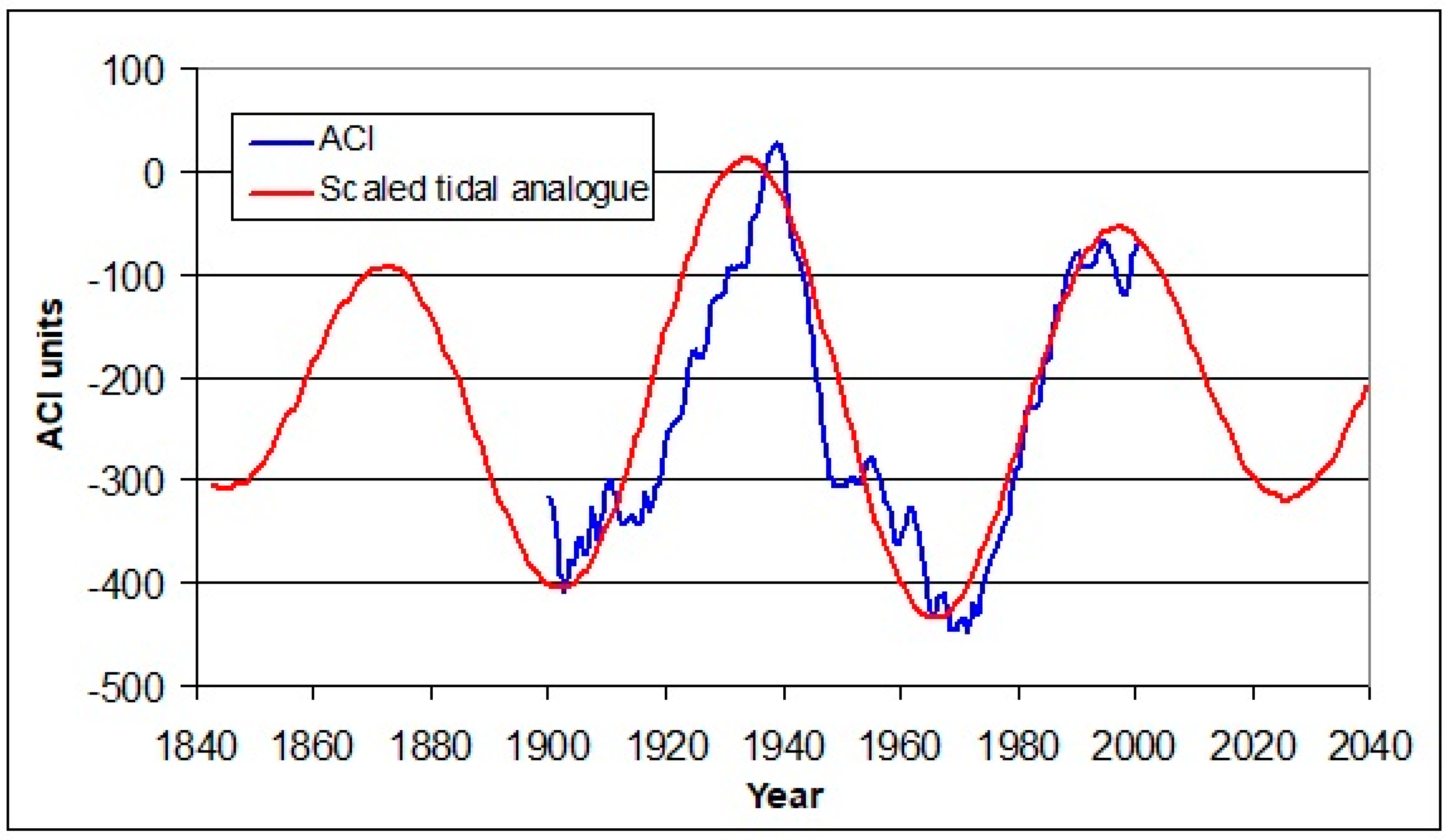
Figure 2.
The accumulated annual Z-M difference from 1500 to 2100 with an eight-year lag, and an analog incorporating the F(t) function.
Figure 2.
The accumulated annual Z-M difference from 1500 to 2100 with an eight-year lag, and an analog incorporating the F(t) function.

Figure 3.
Adding tidal and exponential components to simulate annual unsmoothed HadCRUT4 global mean surface temperature (GMST) anomalies, the curves projected to 2040.
Figure 3.
Adding tidal and exponential components to simulate annual unsmoothed HadCRUT4 global mean surface temperature (GMST) anomalies, the curves projected to 2040.
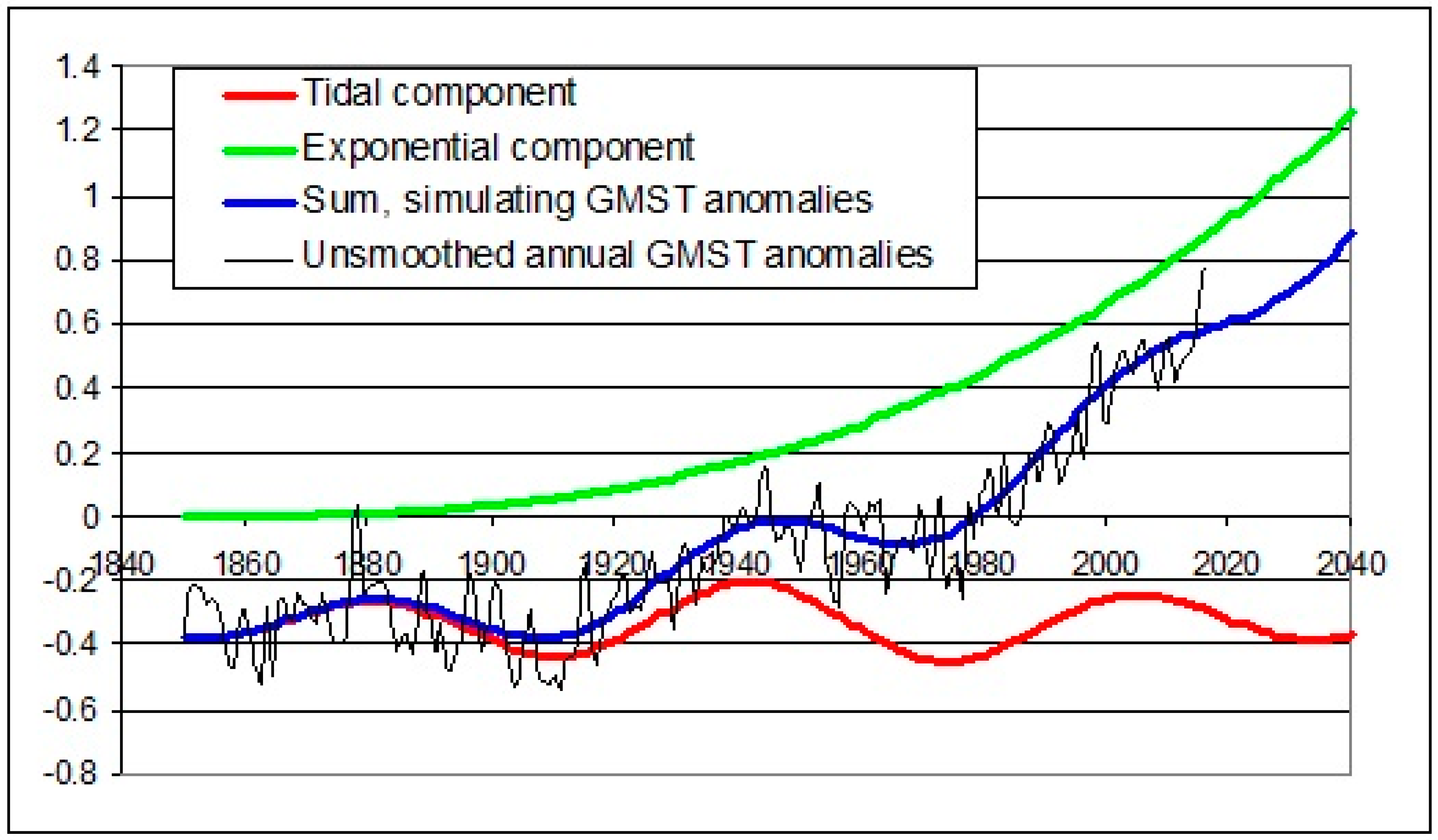
Figure 4.
The mean percent contribution of the exponential component to GMST anomalies on the multidecadal scale after removing a ~60-year tidal oscillation.
Figure 4.
The mean percent contribution of the exponential component to GMST anomalies on the multidecadal scale after removing a ~60-year tidal oscillation.

Figure 5.
Residual HadCRUT4 decadally smoothed anomalies after removing a ~60-year oscillation and an exponential rise in temperature, compared with a sum of 21.70- and 14.94-year tidal components with anomalies lagging the tidal combination by 0.45 years. Residuals calculated from anomalies prone to “end effects” in the smoothing process are labeled “less accurate”.

Figure 6.
The result of adding four regime-dependent components to the previous analysis, compared with residual HadCRUT4 decadally smoothed GMST anomaly residuals, and with anomalies lagging the tidal combination by 0.40 years. Residuals calculated from anomalies prone to “end effects” in the smoothing process are labeled “less accurate”.
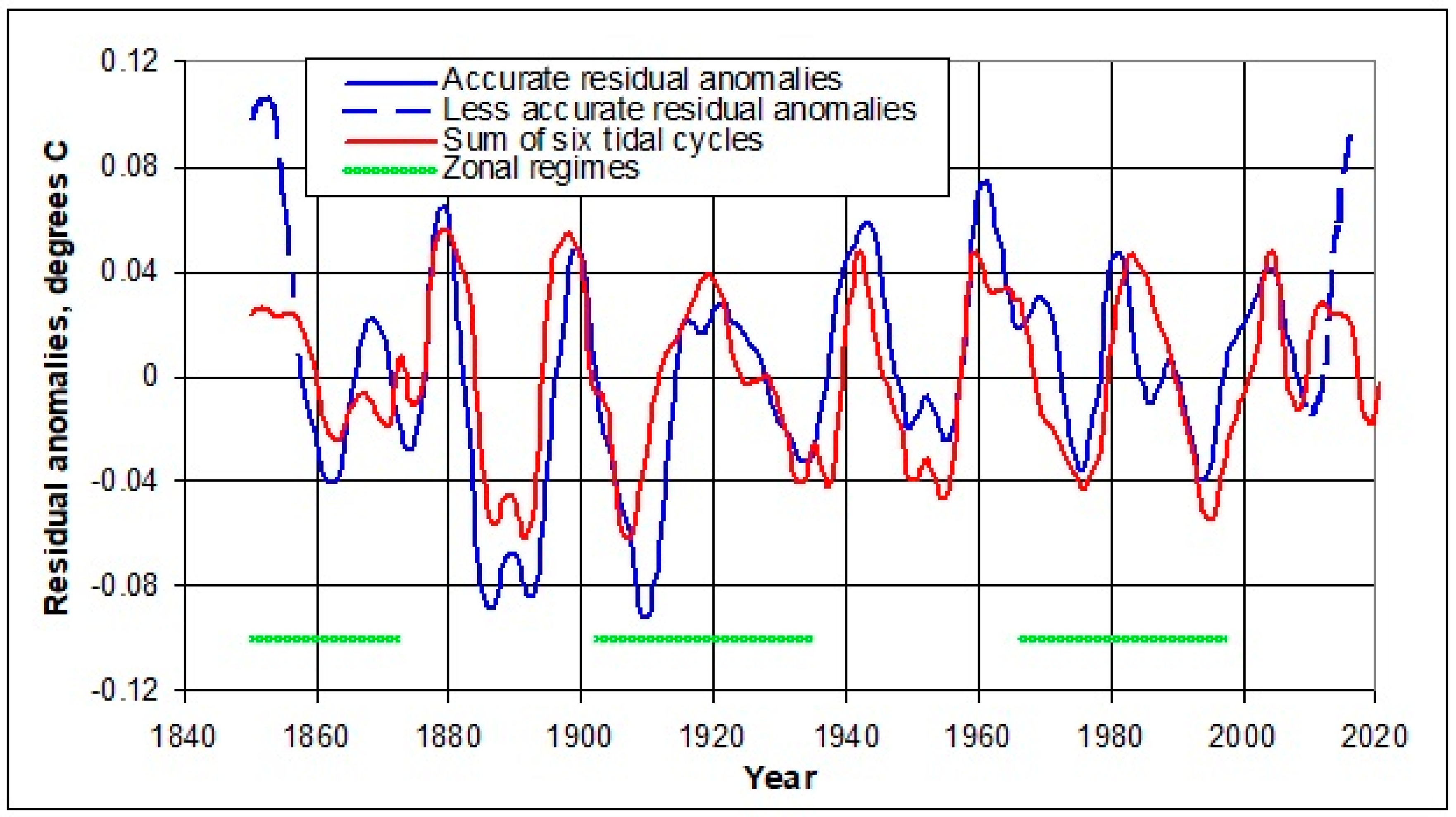
Figure 7.
Root mean square errors (RMSEs) in successive models for decadally smoothed HadCRUT4 anomalies.
Figure 7.
Root mean square errors (RMSEs) in successive models for decadally smoothed HadCRUT4 anomalies.
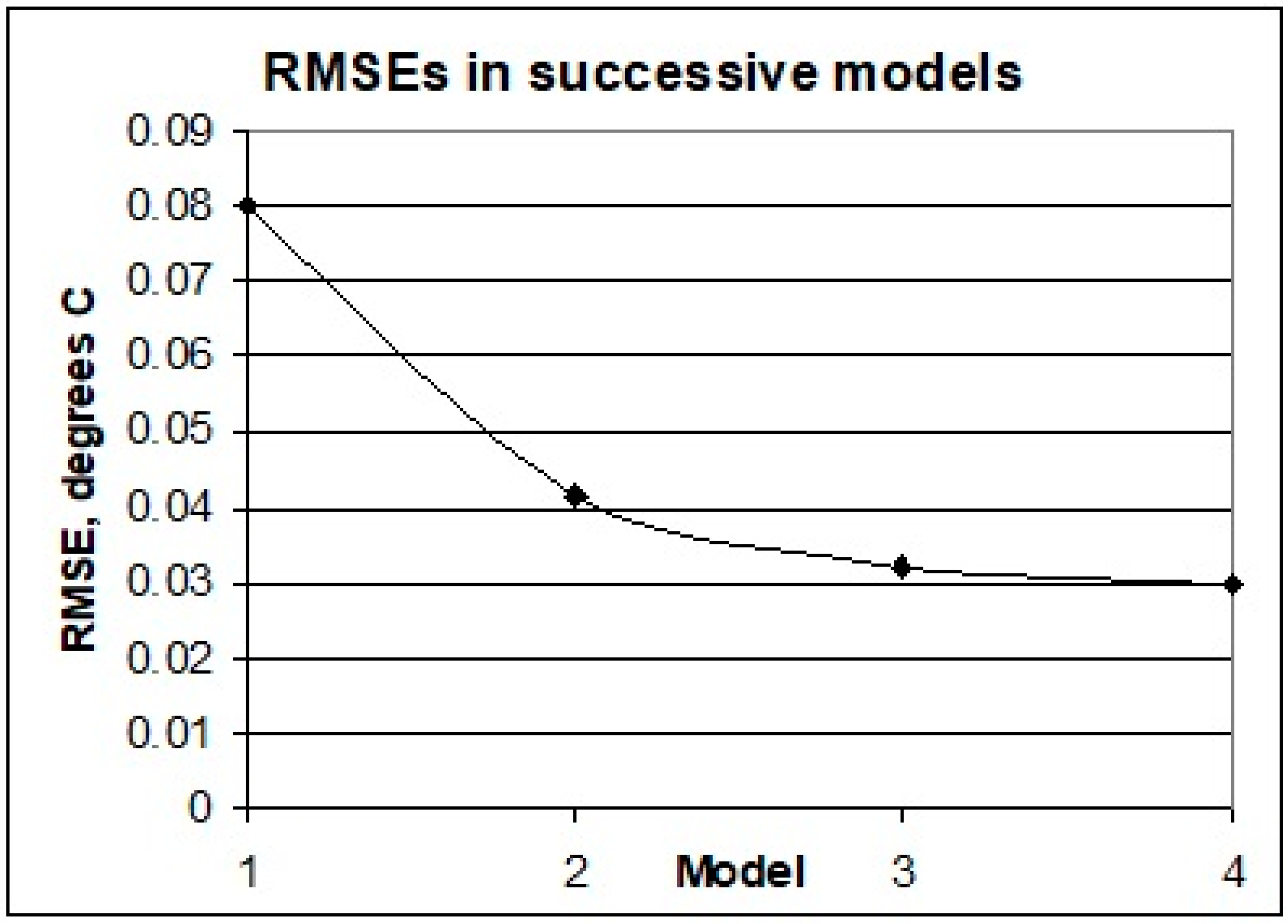
Figure 8.
The scaled temporal variation from 1979 to 2016 of the unsmoothed GMST residual anomalies, detrended UAH lower tropospheric temperatures, and detrended CO2 annual increments and tidal analog. The latter three curves are vertically offset for clarity.
Figure 8.
The scaled temporal variation from 1979 to 2016 of the unsmoothed GMST residual anomalies, detrended UAH lower tropospheric temperatures, and detrended CO2 annual increments and tidal analog. The latter three curves are vertically offset for clarity.
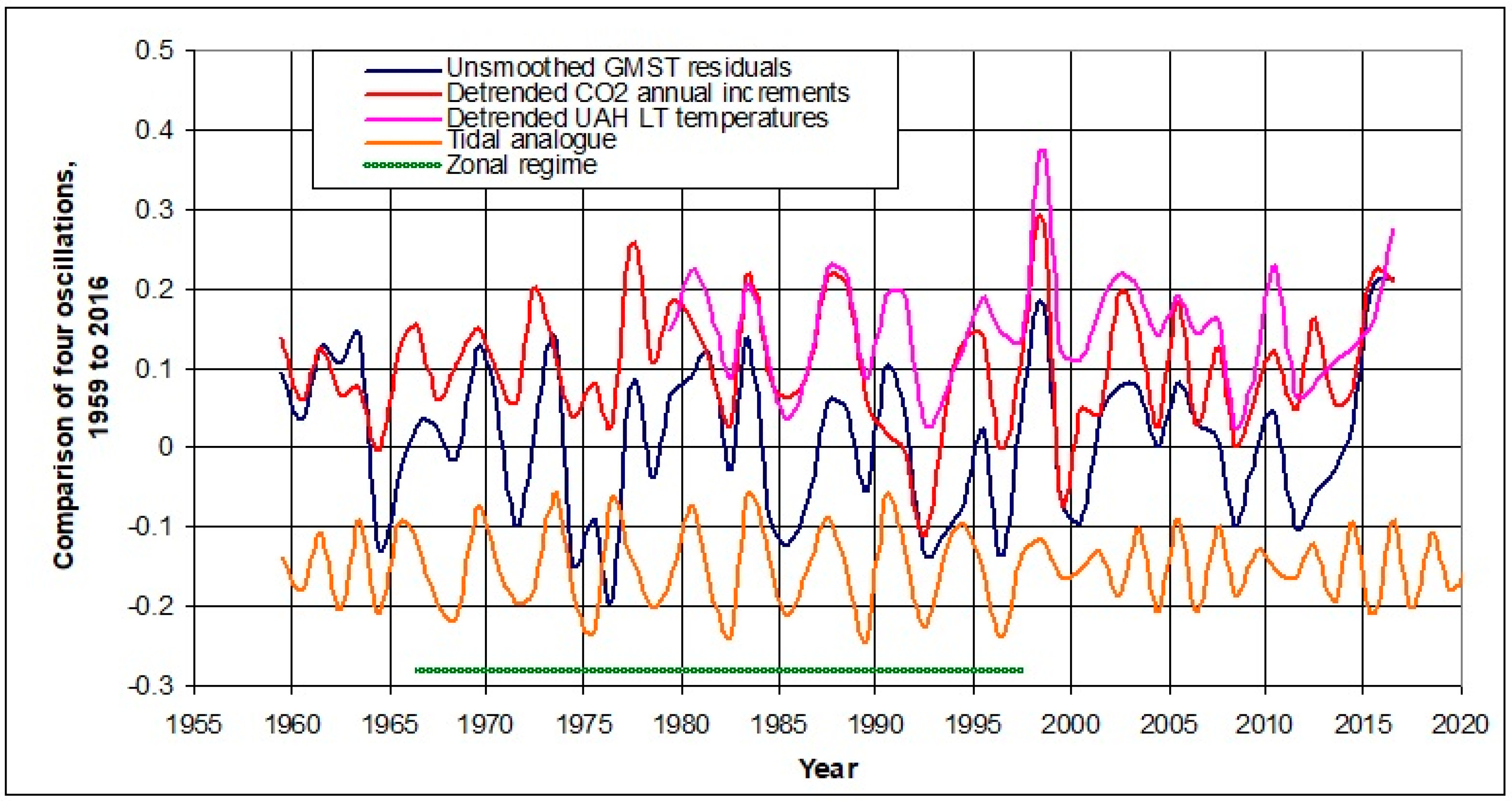
Figure 9.
Comparison of the monthly QBO dataset with the vertically scaled 2.123- and 2.396-year tidal oscillations, with a QBO lag time of 0.15 years.
Figure 9.
Comparison of the monthly QBO dataset with the vertically scaled 2.123- and 2.396-year tidal oscillations, with a QBO lag time of 0.15 years.
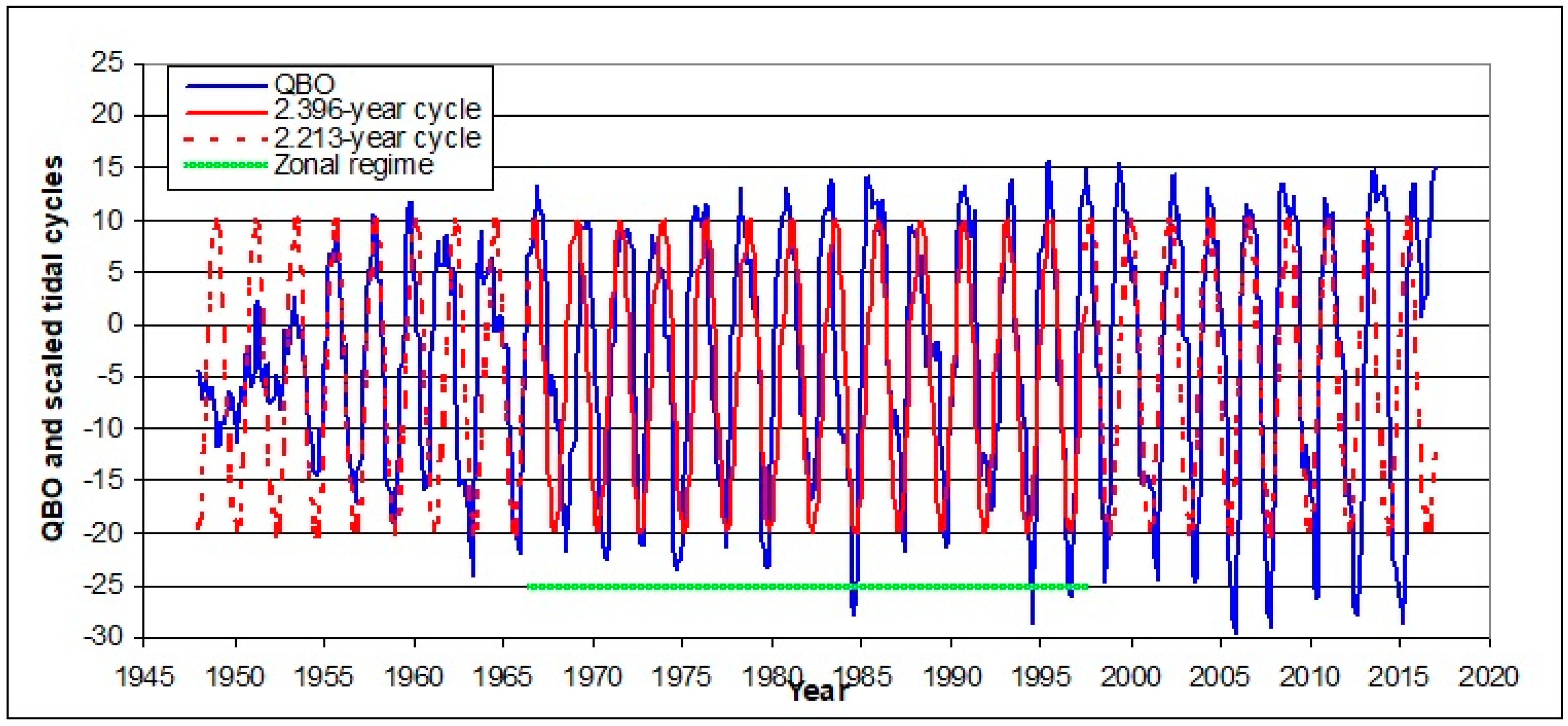
Figure 10.
A comparison of the Oceanic Niño Index with a combination of five subdecadal tidal components.
Figure 10.
A comparison of the Oceanic Niño Index with a combination of five subdecadal tidal components.

Figure 11.
A simulation of the AMO over the time segments: (A) 1856–1940; and (B) 1940–2016, after removing the ~60-year oscillation captured by F(t), and then smoothing with a 13-month running mean. These are compared with a tidal analog, for an AMO lag time of 0.04 years with respect to the tidal analog. The tidal components are listed in Table 13.


Figure 12.
Schematic diagram of suggested steps linking tidal forcing to global climate effects.
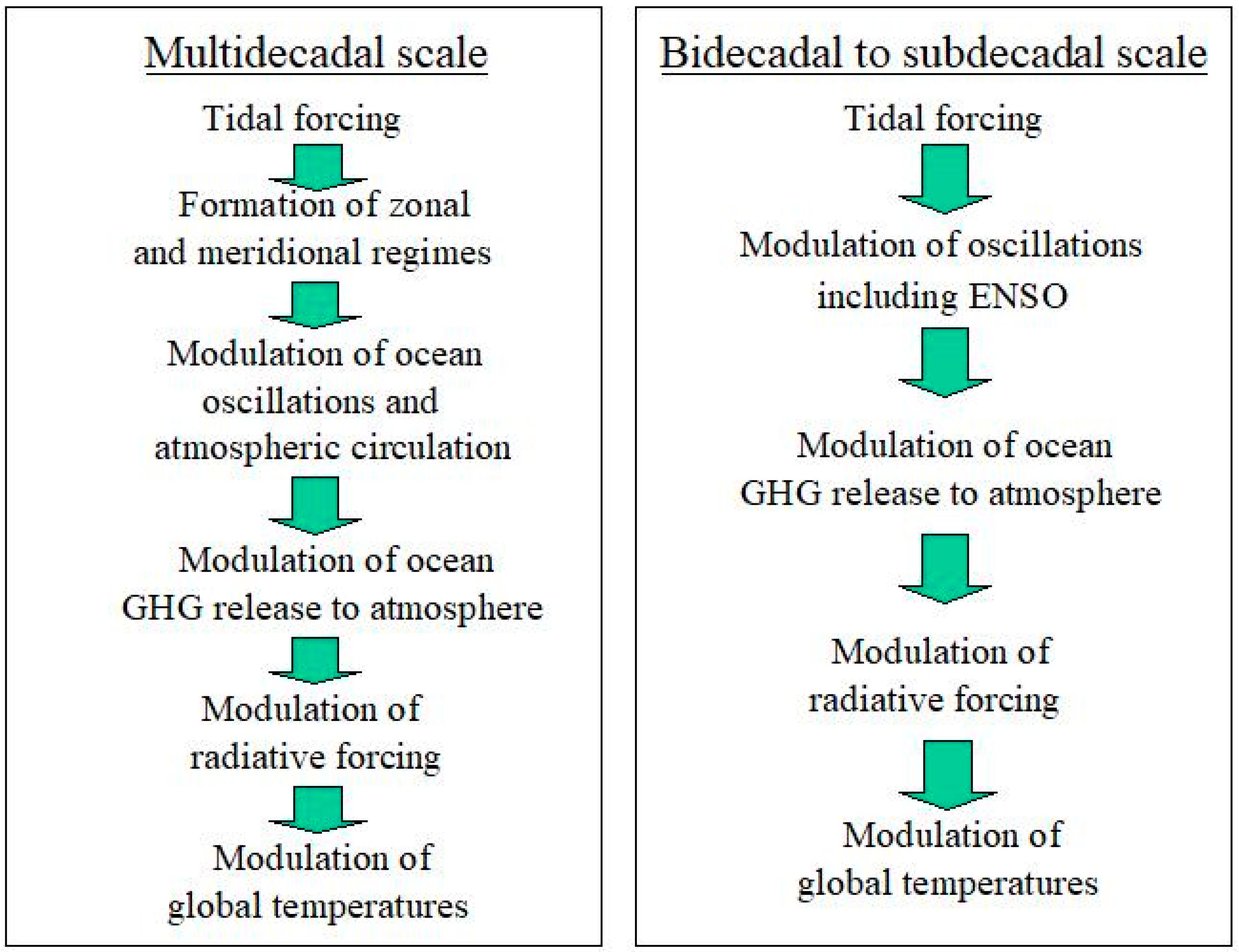

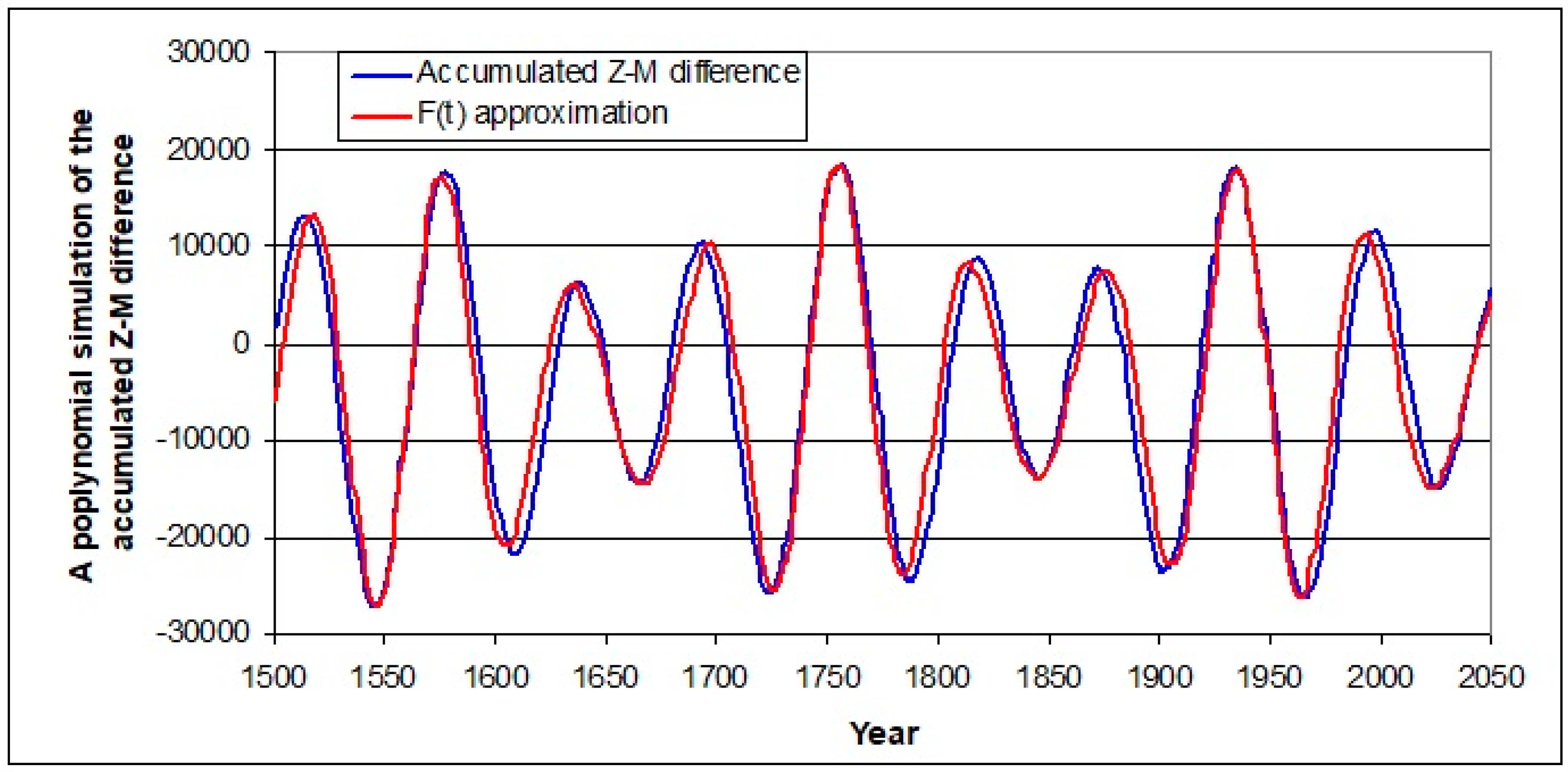
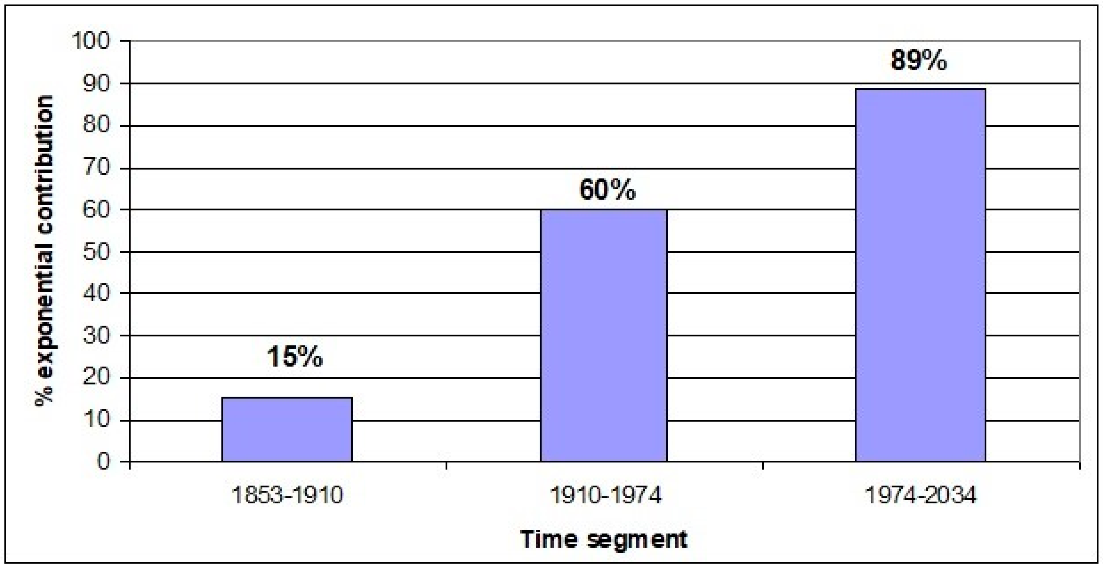
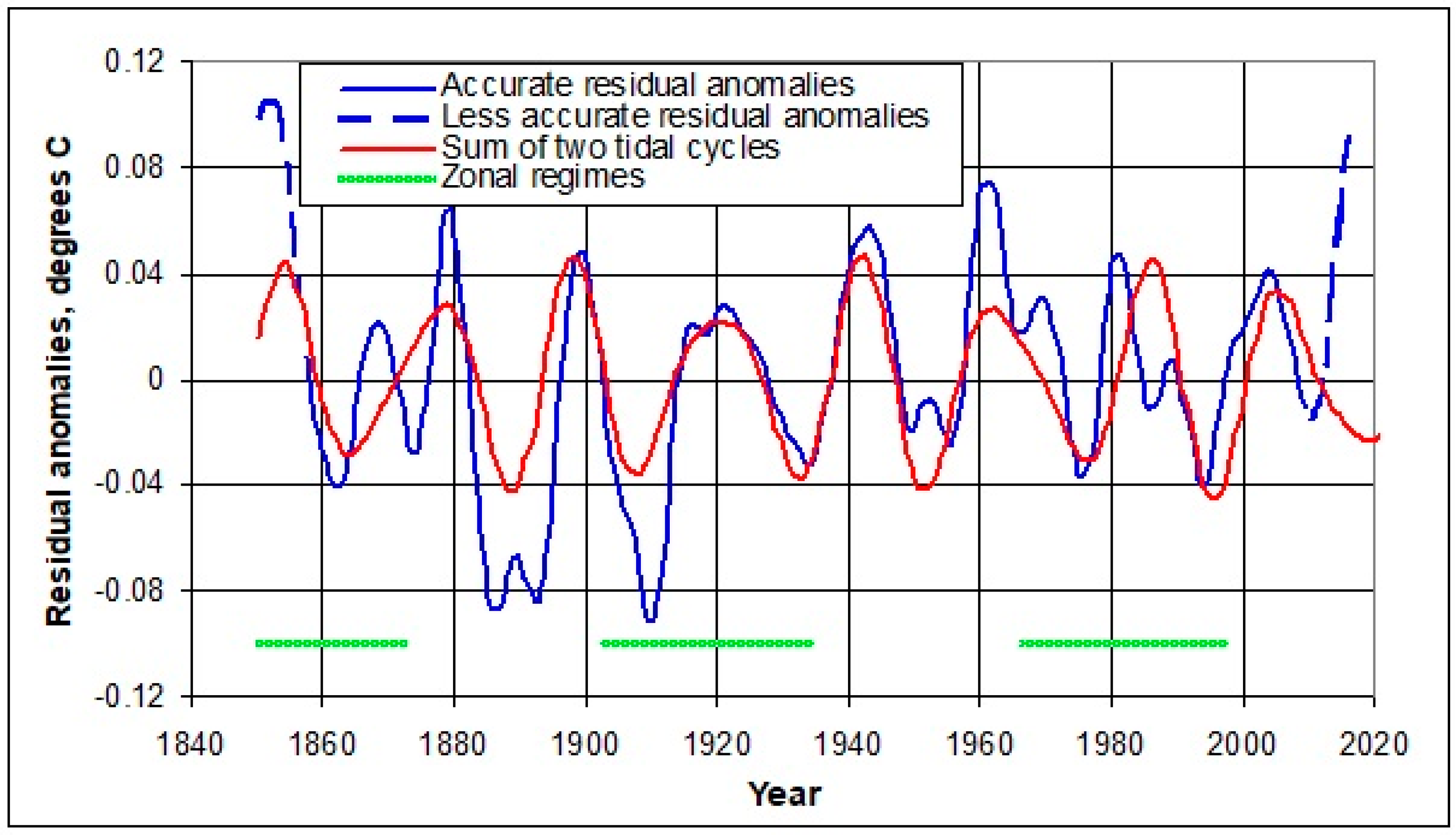
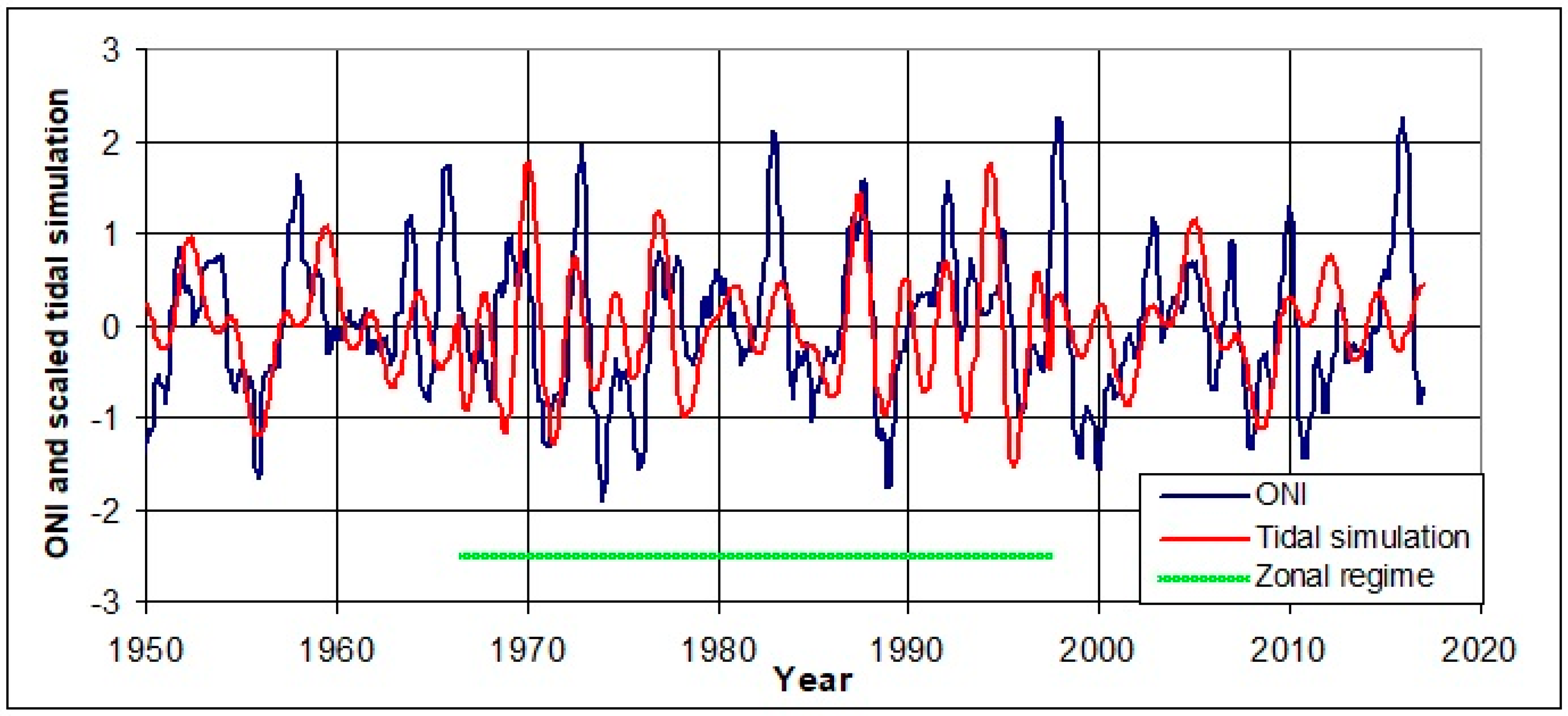
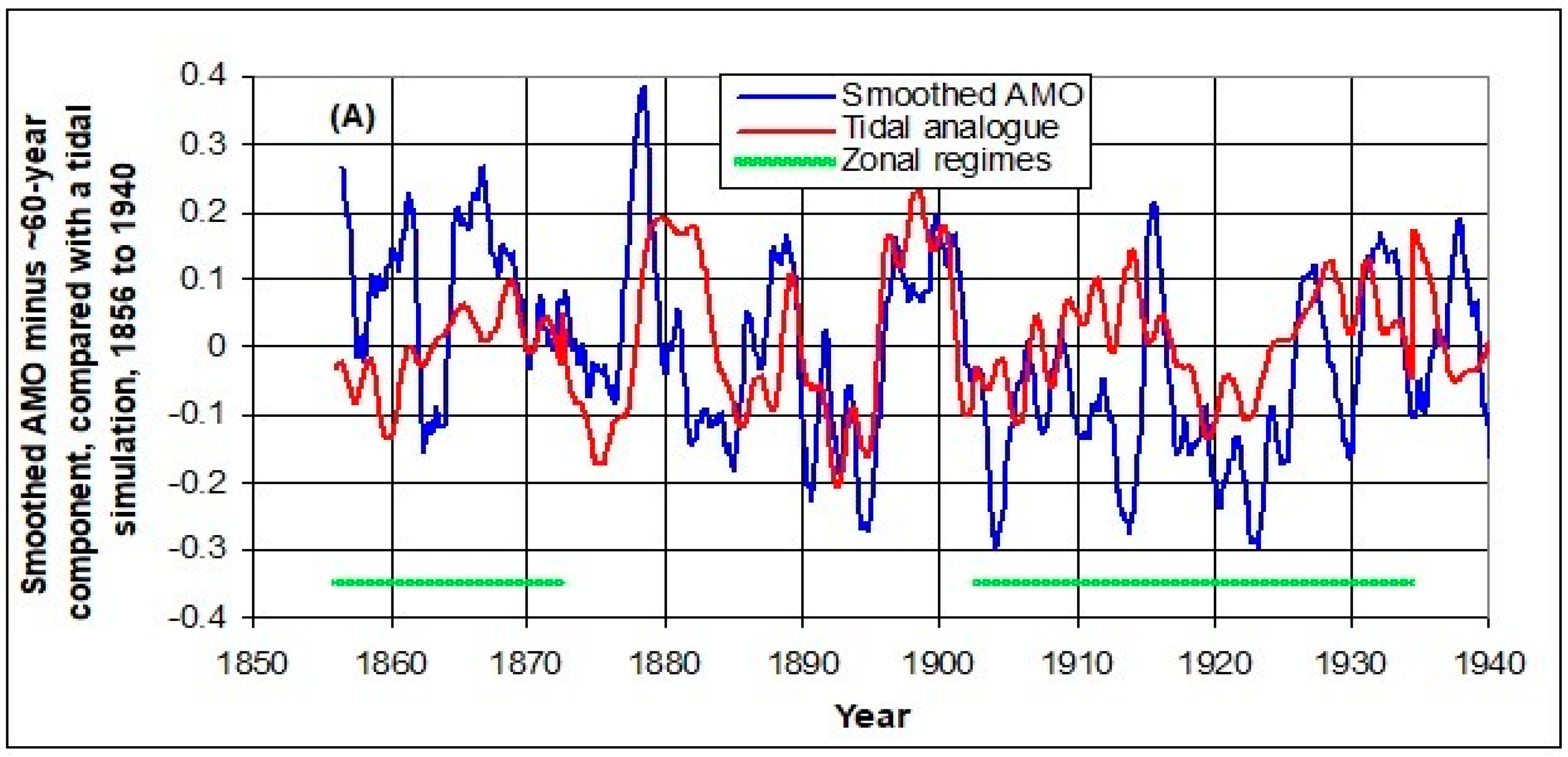
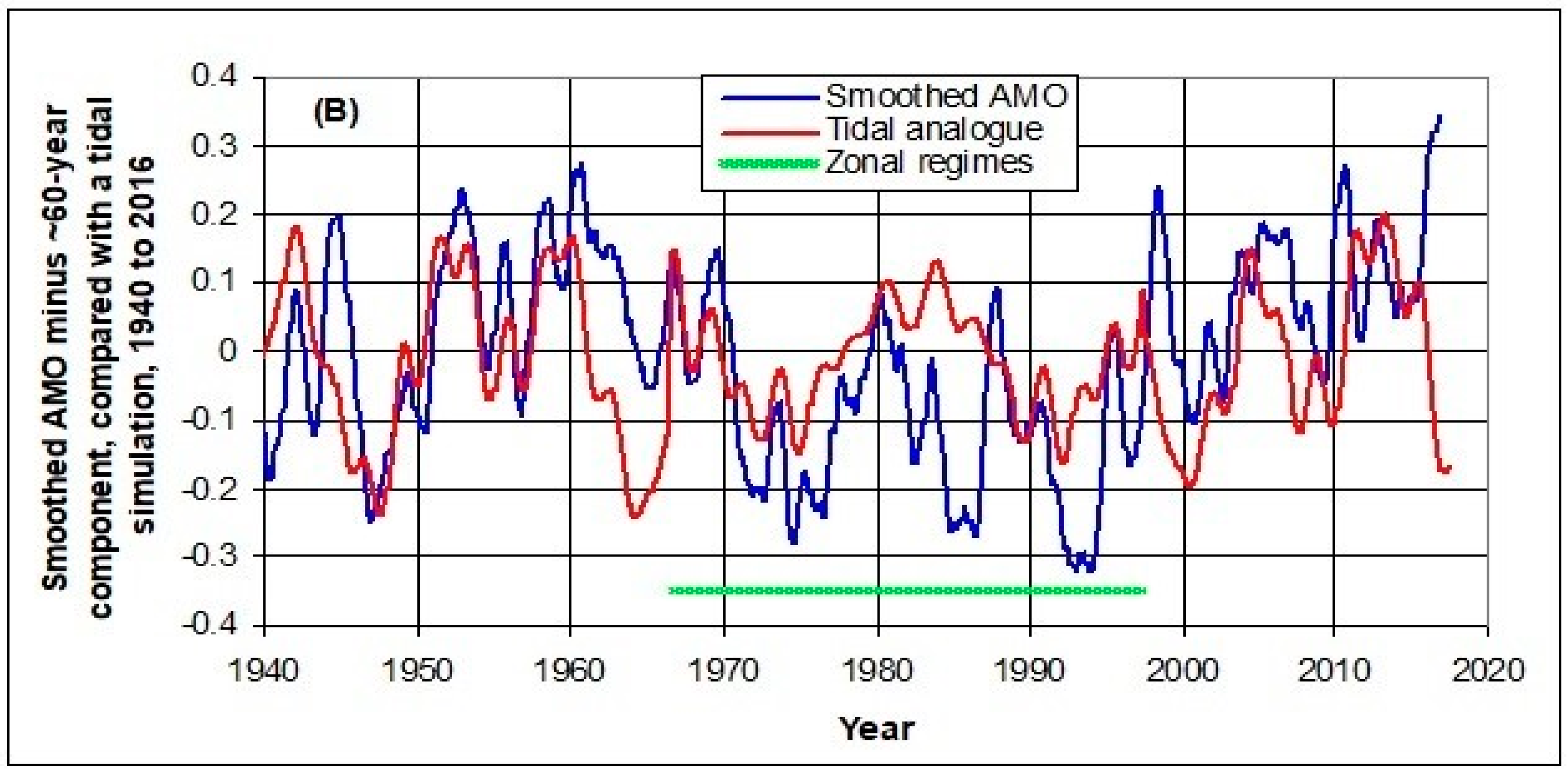
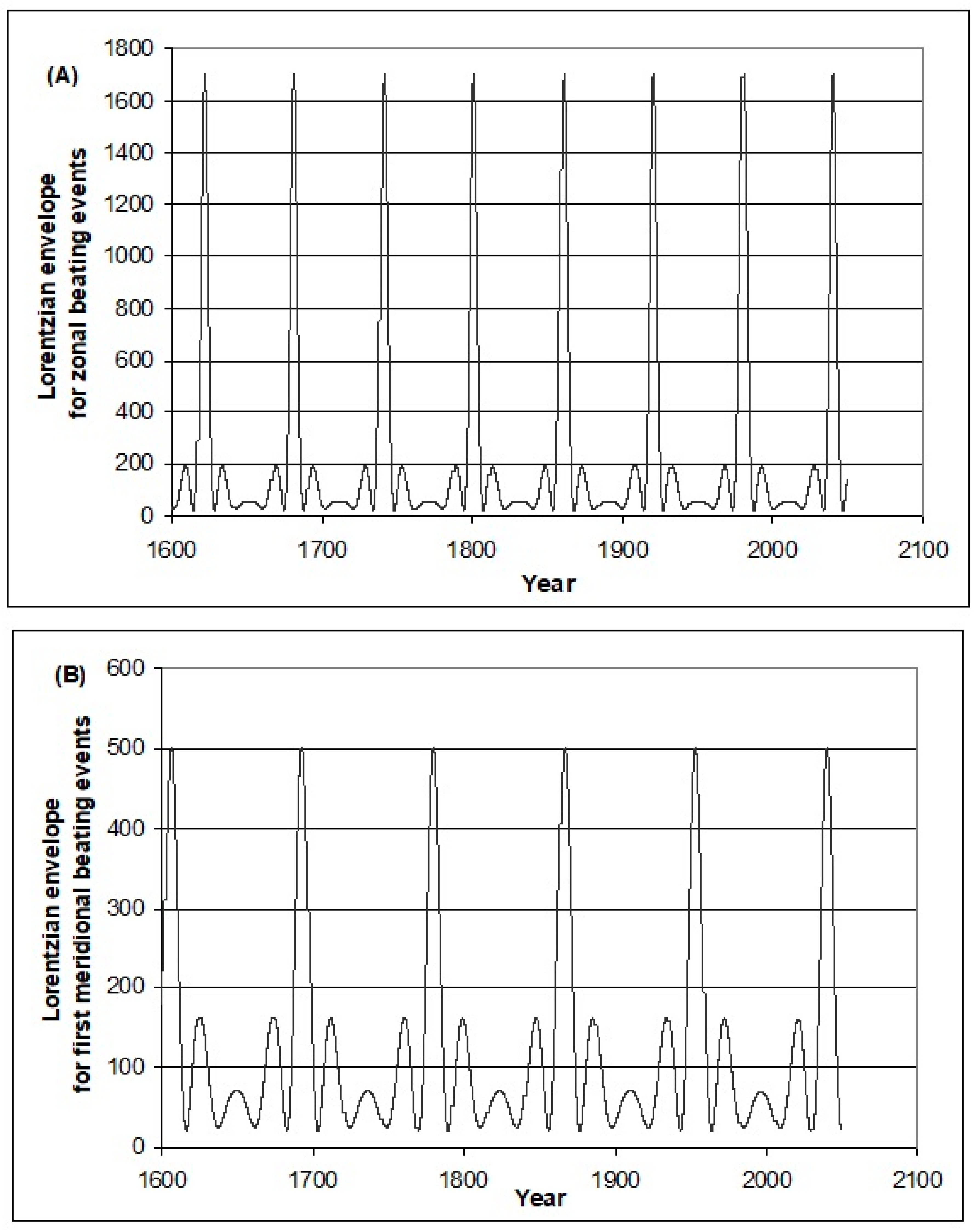
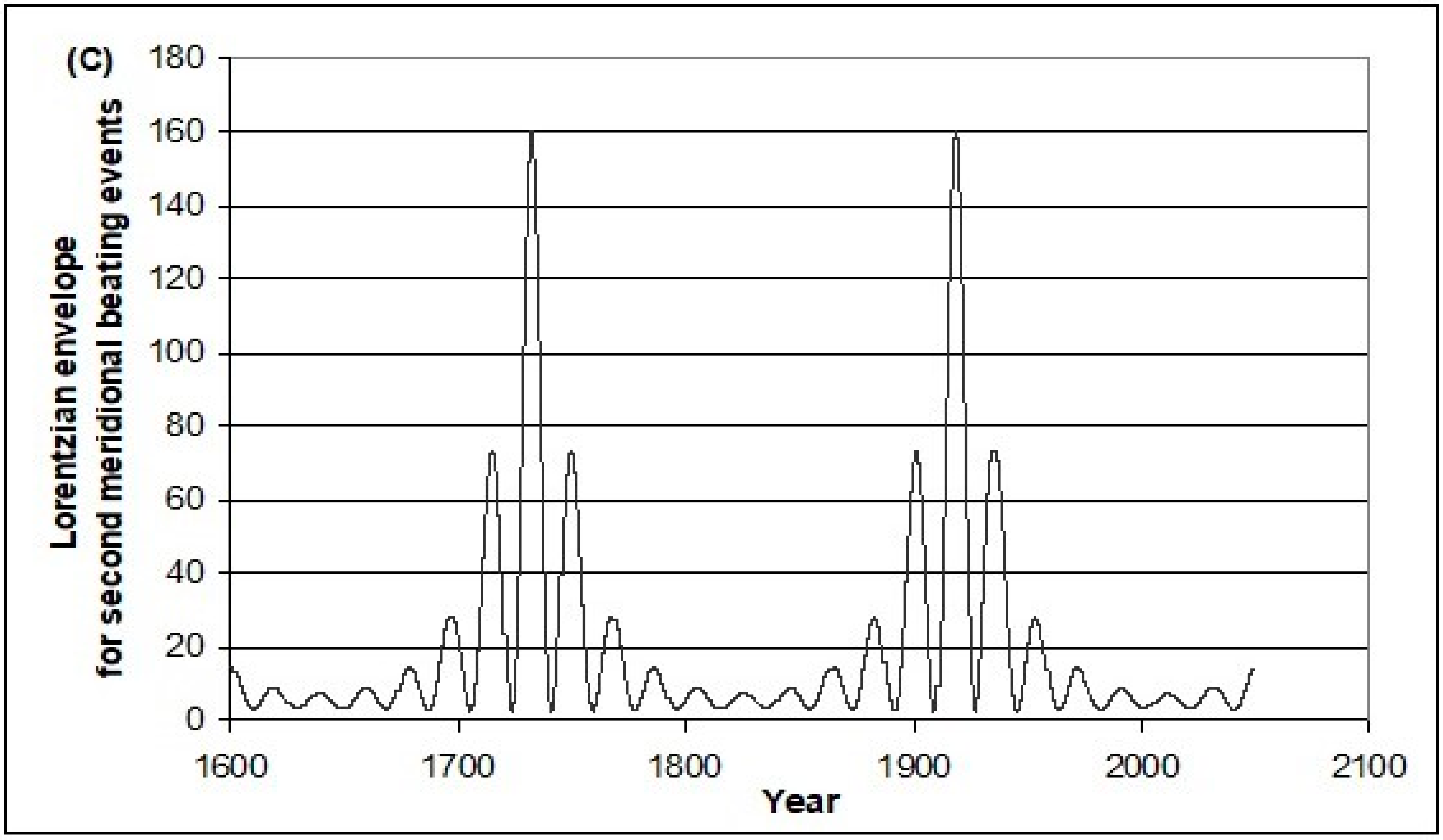
Table 1.
The nature of multidecadal tidal components in this parameterization. Beating amplitudes for the multidecadal cycles are the respective heights of the envelopes shown in the Appendix A.
Table 1.
The nature of multidecadal tidal components in this parameterization. Beating amplitudes for the multidecadal cycles are the respective heights of the envelopes shown in the Appendix A.
| Period P, Years | Frequency Designation | Reference Time, t0 | Beating Amplitude |
|---|---|---|---|
| 59.75 | ν1 | 2039.96 | 1700 |
| 86.81 | ν2 | 2039.96 | 500 |
| 186.0 | ν3 | 1918.20 | 160 |
Table 2.
Intermediate-period (approximately bidecadal) tidal components derived from three fundamental frequency components that are applied to simulate decadally smoothed GMST residual anomalies.
Table 2.
Intermediate-period (approximately bidecadal) tidal components derived from three fundamental frequency components that are applied to simulate decadally smoothed GMST residual anomalies.
| Period P, Years | Frequency Combination | Reference Time, t0 |
|---|---|---|
| 14.94 | ν5 = 4ν1 | 2039.96 |
| 21.70 | ν6 = 4ν2 | 2039.96 |
| 18.60 | ν7 = 10ν3 | 1918.20 |
Table 3.
The 5.778-year component and additional components generated by frequency combination from Table 1 components. The latter four are generated from both zonal and meridional component frequencies.
Table 3.
The 5.778-year component and additional components generated by frequency combination from Table 1 components. The latter four are generated from both zonal and meridional component frequencies.
| Period P, Years | Frequency Combination | Reference Time, t0 |
|---|---|---|
| 5.778 | ν4 | 2039.96 |
| 8.850 | ν8 = ν5 + ν6 = 4ν1 + 4ν2 | 2039.96 |
| 47.92 | ν9 = ν5 − ν6 = 4ν1 − 4ν2 | 2039.96 |
| 3.495 | ν10 = ν4 + ν8 = 4ν1 + 4ν2 + ν4 | 2039.96 |
| 16.69 | ν11 = ν4 − ν8 = 4ν1 + 4ν2 − ν4 | 2039.96 |
Table 4.
Regime-dependent amplitudes for cosine functions for tidal components with a 0.40-year lead time in relation to the decadally smoothed GMST anomaly residuals, in the Figure 6 simulation. The amplitude A entries are in °C for each component, and are given for each period P by with t in decimal years.
| Period P, Years | 21.70 | 14.94 | 8.850 | 47.92 | 16.69 | 5.778 |
|---|---|---|---|---|---|---|
| A (Zonal), °C | −0.04 | −0.01 | −0.01 | −0.005 | −0.015 | 0 |
| A (Meridional), °C | −0.03 | −0.02 | 0.015 | −0.015 | −0.015 | 0.01 |
Table 5.
Statistical results for succeeding models of simulating HadCRUT4 decadally smoothed GMST anomalies.
Table 5.
Statistical results for succeeding models of simulating HadCRUT4 decadally smoothed GMST anomalies.
| Components of Regression | Decadally Smoothed Case: R, RMSE (°C) |
|---|---|
| Model 1. A single exponential factor: 5.0 × 10⁻⁶ (t − 1850.5)2.82 − 0.34 | 0.957, 0.0800 |
| Model 2. The sum of the exponential and the tidal ~60-year oscillation. | 0.988, 0.0418 |
| Model 3. As #2, plus 2 tidal cycles. | 0.994, 0.0321 See Figure 5. |
| Model 4. As #2, plus 6 regime-dependent tidal cycles. | 0.995, 0.0297 See Figure 6 and Table 4. |
Table 6.
Bidecadal tidal components.
| Period P, Years | Frequency Designation | Reference Time, t0 |
|---|---|---|
| 2.396 | ν12 = 4ν8 − 3ν2 = 16ν1 + 13ν2 | 2039.96 |
| 2.213 | ν13 = 4ν8 = 16ν1 + 16ν2 | 2039.96 |
Table 7.
A simulation for tidal component cosine amplitudes (in °C) over the period 1959.5 to 2016.5. The amplitude A entries are in °C for each component, and are given for each period P by Acos(2π[t − 2039.96]/P) with t in decimal years.
Table 7.
A simulation for tidal component cosine amplitudes (in °C) over the period 1959.5 to 2016.5. The amplitude A entries are in °C for each component, and are given for each period P by Acos(2π[t − 2039.96]/P) with t in decimal years.
| Period P, Years | 2.213 | 2.396 | 3.495 |
|---|---|---|---|
| A (Zonal), °C | 0 | −0.03 | 0.08 |
| A (Meridional), °C | −0.06 | 0 | 0 |
Table 8.
Probability p statistics (N = 58) in pair-wise regressions with higher-frequency oscillations from 1959 to 2016. The tidal data are derived from the simulation in Table 7.
Table 8.
Probability p statistics (N = 58) in pair-wise regressions with higher-frequency oscillations from 1959 to 2016. The tidal data are derived from the simulation in Table 7.
| CO2 annual increments | 7.9 × 10⁻⁸ | |
| 3 tidal component simulation | 0.0012 | 0.0026 |
| Unsmoothed GMST residual anomalies | CO2 annual increments |
Table 9.
Probability p statistics (N = 38) in pair-wise regressions of UAH LT temperatures with oscillations from 1979 to 2016. The tidal data are derived from the simulation in Table 7.
Table 9.
Probability p statistics (N = 38) in pair-wise regressions of UAH LT temperatures with oscillations from 1979 to 2016. The tidal data are derived from the simulation in Table 7.
| Unsmoothed GMST residual anomalies | 3.3 × 10⁻¹ |
| CO2 annual increments | 2.3 × 10⁻⁶ |
| 3 tidal component simulation | 0.0020 |
Table 10.
Amplitudes for the five subdecadal tidal components in a simulation of the ONI. The ONI lags the tidal components by 0.22 years.
Table 10.
Amplitudes for the five subdecadal tidal components in a simulation of the ONI. The ONI lags the tidal components by 0.22 years.
| Period, years | 2.213 | 2.396 | 3.495 | 5.778 | 8.850 |
| A (Zonal), °C | −0.6 | 0.5 | 0.5 | 0.3 | 0 |
| A (Meridional), °C | 0 | −0.4 | 0 | 0.4 | 0.4 |
Table 11.
Regime differences for subdecadal tidal components in multiple linear regression statistics with the ONI, for a lag time of 0.22 years.
Table 11.
Regime differences for subdecadal tidal components in multiple linear regression statistics with the ONI, for a lag time of 0.22 years.
| Period, Years | Zonal t | Zonal p | Meridional t | Meridional p |
|---|---|---|---|---|
| 2.213 | −2.7 | 0.0076 | 1.2 | 0.25 |
| 2.396 | 3.8 | 0.00016 | −1.8 | 0.066 |
| 3.495 | 8.5 | 6.1 × 10⁻¹⁶ | 1.7 | 0.088 |
| 5.778 | 2.7 | 0.007 | 4.6 | 5.6 × 10⁻⁵ |
| 8.850 | −0.031 | 0.98 | 4.0 | 6.2 × 10⁻⁵ |
Table 12.
Regime differences in multiple linear regression t and p statistics of subdecadal tidal components against monthly AMO data with lag 0.04 years and after removing the ~60-year oscillation with the F(t) function. Samples: N(zonal) = 954; N(meridional) = 978.
Table 12.
Regime differences in multiple linear regression t and p statistics of subdecadal tidal components against monthly AMO data with lag 0.04 years and after removing the ~60-year oscillation with the F(t) function. Samples: N(zonal) = 954; N(meridional) = 978.
| Period, Years | Zonal t | Zonal p | Meridional t | Meridional p |
|---|---|---|---|---|
| 2.213 | 2.0 | 0.042 | 1.9 | 0.054 |
| 2.396 | −3.6 | 0.00031 | 3.6 | 0.00040 |
| 3.495 | 1.9 | 0.055 | 3.5 | 0.00044 |
| 5.778 | −1.2 | 0.25 | 2.8 | 0.0050 |
| 8.850 | 1.6 | 0.10 | 6.9 | 7.8 × 10⁻¹² |
| 14.94 | −1.9 | 0.064 | 0.47 | 0.64 |
| 16.69 | −6.9 | 9.6 × 10⁻¹² | 1.1 | 0.26 |
| 18.60 | −3.7 | 0.00026 | 4.6 | 5.6 × 10⁻⁶ |
| 21.70 | 0.50 | 0.62 | −2.0 | −0.044 |
Table 13.
Regime-dependent component amplitudes A in a simulation of the AMO after removing a ~60-year oscillation. The AMO lags tidal components by 0.04 years.
Table 13.
Regime-dependent component amplitudes A in a simulation of the AMO after removing a ~60-year oscillation. The AMO lags tidal components by 0.04 years.
| Period, Years | 2.213 | 2.396 | 3.495 | 5.778 | 8.850 | 14.94 | 16.69 | 18.60 | 21.70 |
| A (Zonal), °C | 0.02 | −0.03 | 0.03 | −0.01 | 0.01 | −0.02 | −0.06 | −0.05 | 0.00 |
| A (Meridional), °C | 0.03 | 0.03 | 0.03 | 0.02 | 0.12 | 0.00 | 0.00 | 0.09 | −0.02 |
Table 14.
Tidal frequency components in climate oscillations examined in this paper. The penultimate column lists the regime in which the components show greatest responses in the climate oscillations discussed.
Table 14.
Tidal frequency components in climate oscillations examined in this paper. The penultimate column lists the regime in which the components show greatest responses in the climate oscillations discussed.
| Frequency Designation | Period, Years | Frequency Combination | Representation for ν1 ν2 ν3 ν4 | Main Active Regime | t0 (AD) |
|---|---|---|---|---|---|
| ν1 | 59.75 | ν1 | 1000 | Zonal | 2039.96 |
| ν2 | 86.81 | ν2 | 0100 | Meridional | 2039.96 |
| ν3 | 186.0 | ν3 | 0010 | Meridional | 1918.20 |
| ν4 | 5.778 | ν4 | 0001 | Meridional | 2039.96 |
| ν5 | 14.94 | 4ν1 | 4000 | Both | 2039.96 |
| ν6 | 21.70 | 4ν2 | 0400 | Both | 2039.96 |
| ν7 | 18.60 | 10ν3 | 00(10)0 | Meridional | 1918.20 |
| ν8 | 8.850 | 4ν1 + 4ν2 | 4400 | Meridional | 2039.96 |
| ν9 | 47.92 | 4ν1 − 4ν2 | 4-400 | Both | 2039.96 |
| ν10 | 3.495 | 4ν1 + 4ν2 + ν4 | 4401 | Both | 2039.96 |
| ν11 | 16.69 | 4ν1 + 4ν2 − ν4 | 440-1 | Zonal | 2039.96 |
| ν12 | 2.396 | 16ν1 + 13ν2 | (16)(13)00 | Zonal | 2039.96 |
| ν13 | 2.213 | 16ν1 + 16ν2 | (16)(16)00 | Meridional | 2039.96 |
© 2017 by the author. Licensee MDPI, Basel, Switzerland. This article is an open access article distributed under the terms and conditions of the Creative Commons Attribution (CC BY) license (http://creativecommons.org/licenses/by/4.0/).
Share and Cite
MDPI and ACS Style
Treloar, N.C. Deconstructing Global Temperature Anomalies: An Hypothesis. Climate 2017, 5, 83. https://doi.org/10.3390/cli5040083
AMA Style
Treloar NC. Deconstructing Global Temperature Anomalies: An Hypothesis. Climate. 2017; 5(4):83. https://doi.org/10.3390/cli5040083
Chicago/Turabian StyleTreloar, Norman C. 2017. "Deconstructing Global Temperature Anomalies: An Hypothesis" Climate 5, no. 4: 83. https://doi.org/10.3390/cli5040083
Note that from the first issue of 2016, this journal uses article numbers instead of page numbers. See further details here.