
Influence of Urban Green Area on Air Temperature of Surrounding Built-Up Area


Department of Architecture, Kobe University, Kobe 657-8501, Japan
Climate 2017, 5(3), 60; https://doi.org/10.3390/cli5030060
Submission received: 17 July 2017
/
Revised: 2 August 2017
/
Accepted: 2 August 2017
/
Published: 7 August 2017
(This article belongs to the Special Issue Urban Overheating - Progress on Mitigation Science and Engineering Applications)
Abstract
:In this investigation, a numerical model expressing advection and diffusion effects is used to examine air temperature rise in urban areas that are on the leeward side of green areas. The model results are then verified by comparison with measurement results. When the measurement point is at a distance of 30 m or more from a green area, the air temperature of the urban area is not affected by the green area. An isotropic diffusion model and a model incorporating buoyancy were applied for the vertical diffusion term. Results of air temperature rise with distance from the green area were compared for both calculated and measured values. The rise in air temperature due to the development of the urban boundary layer in the area near a green space is expressed using the sensible heat flux from the ground surface, the distance from the green area and the wind velocity. We considered an approximation of air temperature rise in order to express the following situation: when entering the urban area, air temperature rises sharply, and when reaching a certain distance from a green area, it becomes almost constant.
1. Introduction
Urban greenery is one of the main measures for mitigating the thermal environment in urban spaces. Givoni [1] has organized the functions and impacts of urban planted areas through a review of research papers and has presented climatic guidelines for hot-dry regions, hot-humid regions and cold regions. A summary of climatic guidelines for park design is as follows: it is to provide ample shade and to protect from dust for hot-dry regions; it is to provide shade, to minimize wind blockage, to improve the ventilation and to minimize floods for hot-humid regions; it is to provide wind protection without blocking the winter sun for cold regions. He summarized that the influence of city parks and open spaces on the urban climate is limited to the conditions prevailing within these areas themselves, and extends only a short distance into the surrounding, densely built, urban area. On the other hand, Honjo and Takakura [2] explained that the range of the effects of urban green areas extends to about 100 to 300 m into the surrounding urban area. They also explained that 300 m along the main wind direction is the ideal length for an urban green area, based on two-dimensional analysis results.
In recent years, interest in this field of study has increased. How to quantify the range of the air temperature reduction effect of an urban green area on the surrounding urban area is a question that has been frequently asked by administrative officials responsible for organizing urban green spaces. Moriyama et al. [3] have conducted numerical simulations to examine increases and decreases in air temperature in urban areas adjacent to green areas. They used the following conditions: an inflow upper wind velocity of 2 to 6 m/s at 50 m above the ground, a ground surface temperature difference of 1 to 5 °C between green and urban areas, and a roughness parameter of 0.1 to 1.0 m for green areas and 0.5 to 1.0 m for urban areas. The evaluation height was 3.25 m above the ground. They concluded that the influence of the green space extends to a distance of about 150 m from the urban-green boundary. The above-mentioned Honjo et al. [2] have carried out numerical simulations under the condition that an inflow upper wind velocity is 4 m/s at 200 m above the ground, a ground surface temperature difference is 4 °C between green and urban areas, and a roughness parameter is 0.2 m for both the green area and the urban area. The evaluation height in this case was 2 m above the ground. They concluded that even a green area with 100 m size affects the area within a distance of about 300 m from the urban-green boundary.
There are a few studies focusing on air temperature reduction in urban areas around a green area [4]. Ca et al. [5] have carried out field measurements to determine the cooling influence of a park on the surrounding area in the Tama New Town, a city in the west of Tokyo. With the size of 0.6 km2, a park can reduce the air temperature by up to 1.5 °C at noon time in a leeward commercial area at distance of 1 km. Yu and Hien [6] have carried out temperature and humidity measurements in two big city green areas (36 ha and 12 ha) in Singapore. A three-dimensional non-hydrostatic model (Envi-met) was applied for the simulation of Surface-Plant-Air interactions inside urban environments. Horizontal air temperature profiles in both the green area and surrounding area are calculated by the Envi-met model.
Yagi and Takebayashi [7] have performed measurements at four urban areas in Kobe City. The spatial variation of the vertical air temperature gradient between 4.0 m and 1.5 m is large in urban areas, since air temperature reduction effect in urban areas is different depending on the circumstances around the measurement point. Since sea breezes dominate in summer days in many cities in Japan, air temperature reduction due to advection effects is expected in regions leeward of urban green areas. In this study, the characteristics of air temperature in the urban area on the leeward side of green areas are considered using a numerical model incorporating advection and diffusion, and verified by comparison with measurement. The objective of this study is to clarify the characteristics of air temperature rise in an urban area on the leeward side of a green area, as a contribution to the practical planning of urban greening.
2. Measurements
2.1. Study Site
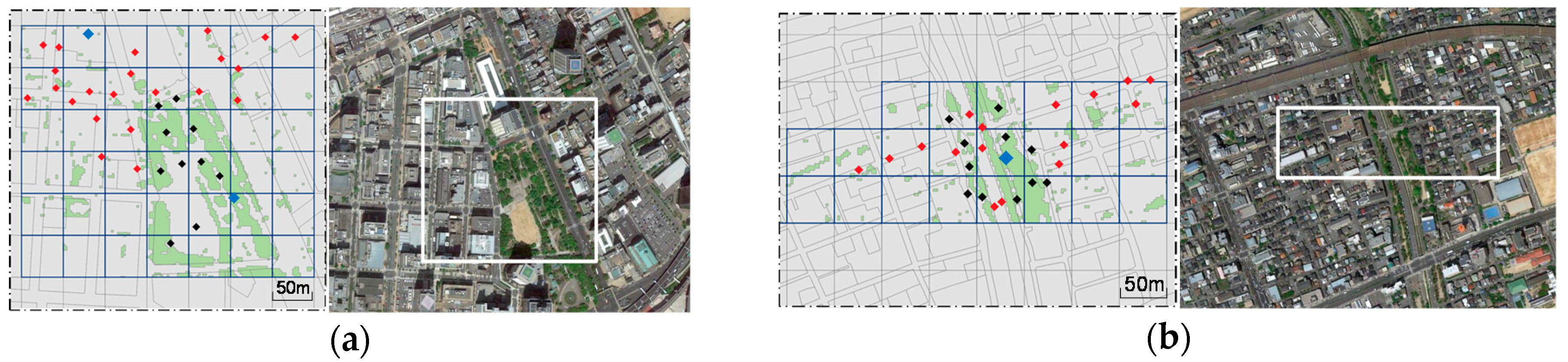
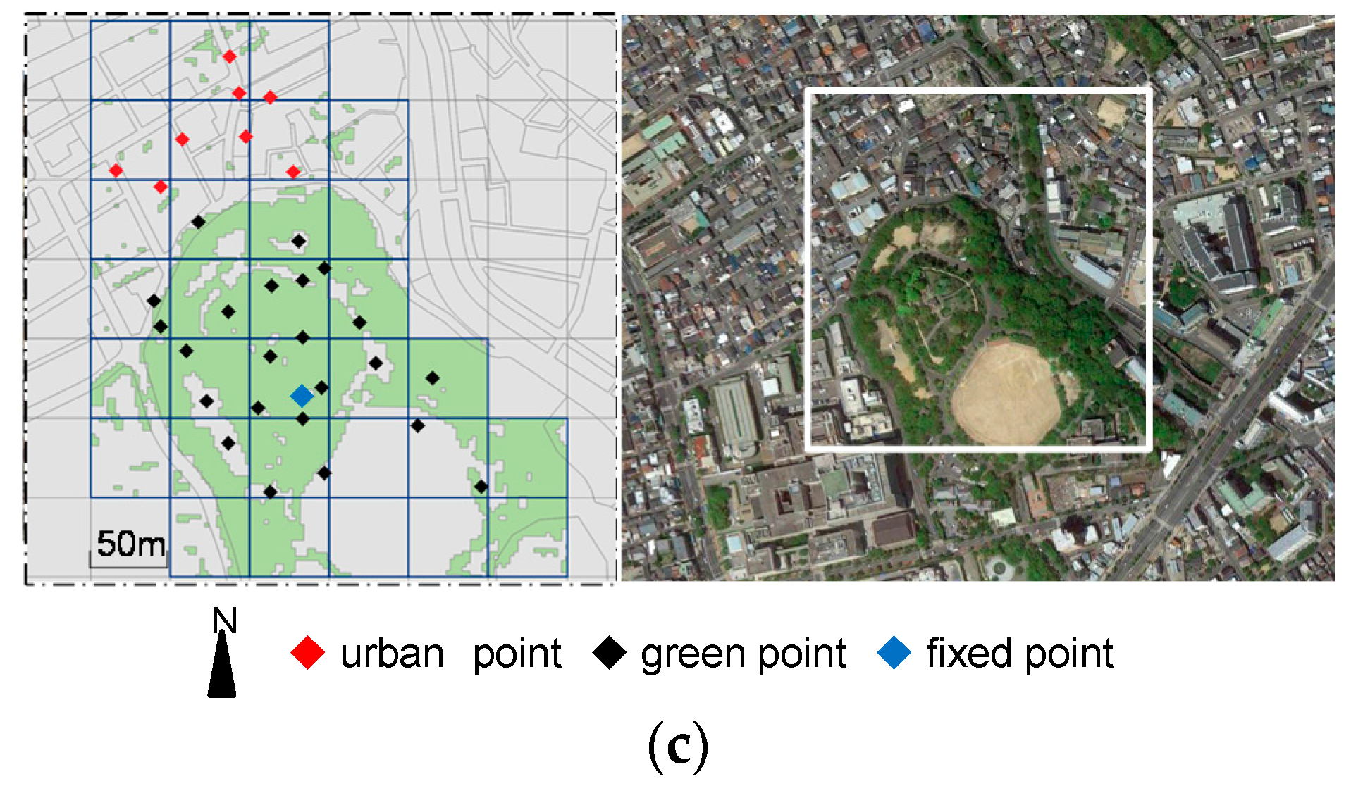
Mobile measurements were carried out in Higashi-yuen Park (about 2.7 ha, green coverage rate, which is the ratio of the canopy area to the park area: about 45%) and a neighboring business area at 13:00 and 17:00 on 2 August 2012, in Ishiyagawa Park (about 4 ha, green coverage ratio: about 42%) and a residential area at 13:00 and 17:00 on 4 August 2012, and in Okurayama Park (about 7.9 ha, green coverage ratio: about 70%) and a residential area at 13:00 and 17:00 on 8 August 2012. These parks are all located in Kobe city, Japan. Mobile measurement points and aerial photographs are shown in Figure 1. The grid lines are spaced 50 m apart. The green color indicates green coverage.
Higashi-yuen Park and the business area are located in the center of Kobe City. There are public buildings such as Kobe City Hall and general offices etc. in the business area. Middle-high-rise buildings are dominant. Ishiyagawa Park and the neighboring residential area are located in an urban area at the southern foot of Rokko Mountain on the east side of Kobe City. There are mainly detached houses and small scale collective houses in the residential area. Low-rise buildings are dominant. Okurayama Park and its residential area are located in the urban area at the southern foot of Rokko Mountain on the west side of Kobe City. There are detached houses, hospitals, etc. in the residential area. Low-rise building and middle-rise building are mixed.
2.2. Outline of Measurements
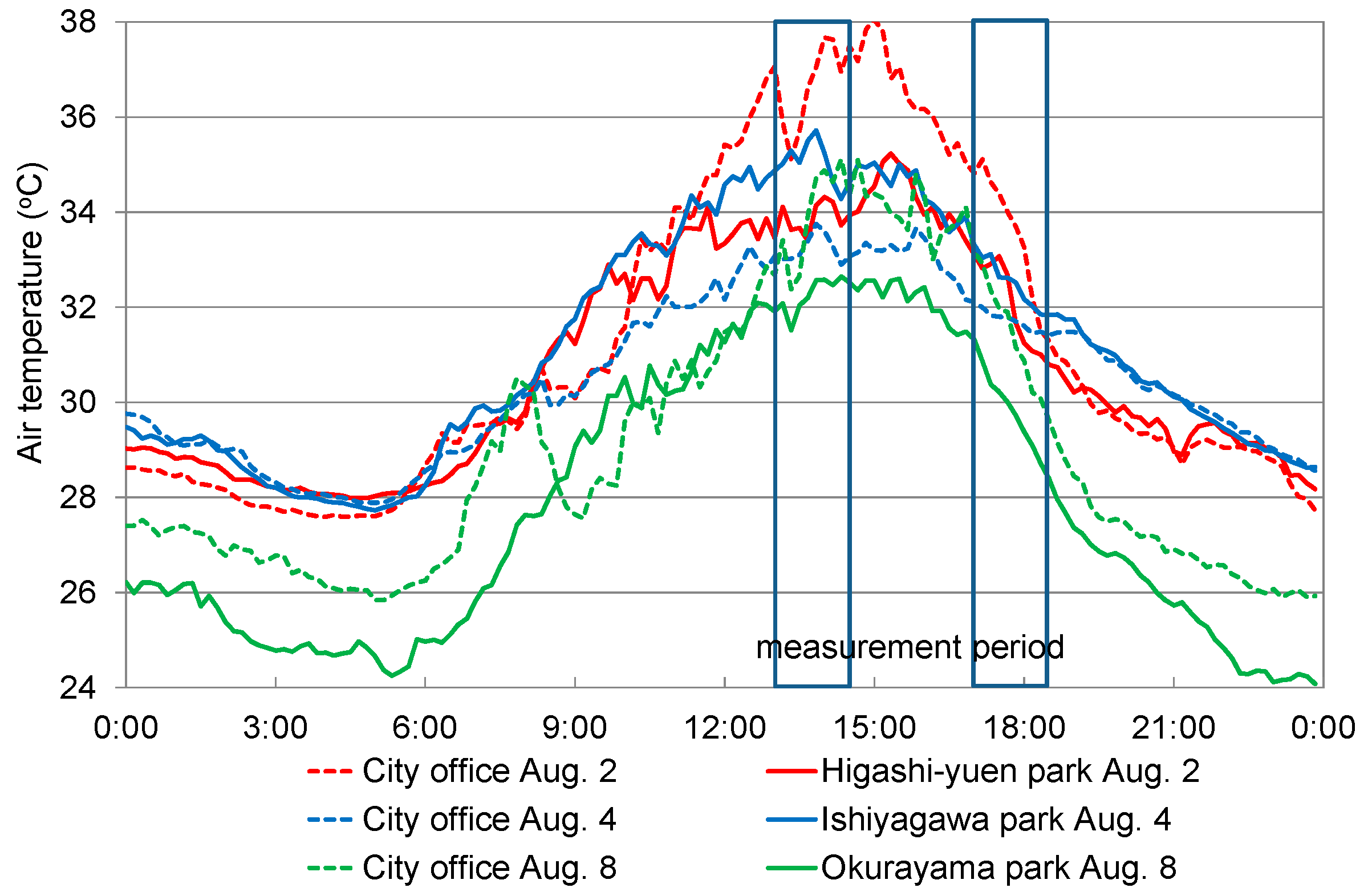
The elements measured are air temperature, wind direction, wind velocity at a height of 1.5 m, and surface temperature. The measuring device and method are shown in Table 1. Wind velocity was sampled every second at each mobile measurement point which is indicated as an urban point and green point in Figure 1 and the averaged value for 30 s was recorded. Wind direction was recorded based on the direction with the highest frequency in the 30 s. Measurement results for air temperature at the fixed measurement points are shown in Figure 2. It was continuously measured only at fixed points. Thermistor sensors were installed in a natural ventilation-type solar radiation shielding device and were set on the roof of the Kobe City Hall No. 3 building (47 m above the ground, flat concrete roof with the usual waterproof sheet finish) and the trunks of trees in the Higashi-yuen Park, Ishiyagawa Park, and Okurayama Park (3 m above the ground). Kobe City Hall and Higashi-yuen Park are close to each other. The distances from Ishiyagawa Park and Okurayama Park to Kobe City Hall are about 5.7 km and 2.1 km, respectively.
Although it took a maximum of 1.5 h for the mobile measurements at each site to be made, no sudden changes in weather were confirmed as compared with the results of the fixed-point measurements, so no correction was made to the results of the mobile measurements. For the analysis in the next section, I used the difference between air temperature from the mobile measurements in the urban area and the air temperature of the fixed-point measurements in the park at that time.
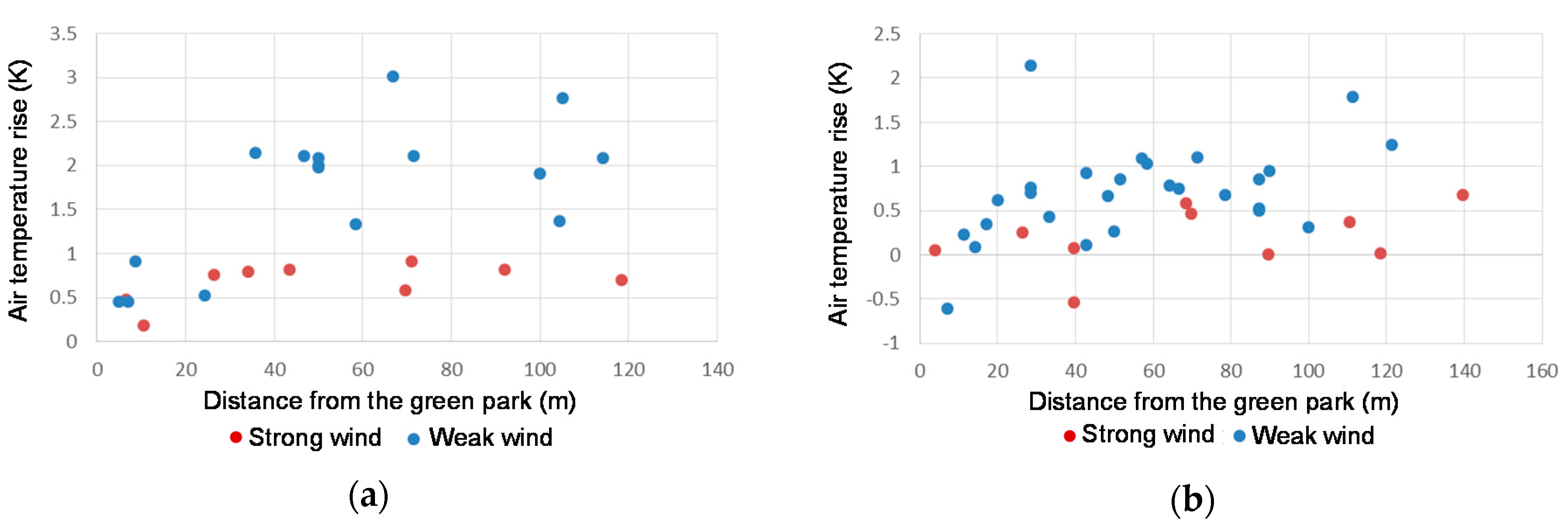
The boundary between the green area and the urban area is set to 0, and the following analysis is carried out, focusing on the relationship between the horizontal distance from the boundary and the air temperature in the urban areas. Since the main wind direction was southwest in the case of measurements around Higashi-yuen Park, the measurement results in the northeastern urban area were used for analysis. The distance to the park was calculated by drawing a straight line in the southwest direction from each mobile measurement point. Similarly, since the main wind direction was east in the case of measurements around Ishiyagawa Park, the measurement results in the west urban area were used for analysis. In the case of measurements around Okurayama Park, the main wind direction was south-southeast, so the measurement results in the northern urban area were used for analysis. Figure 3 shows the distance from the green area to each mobile measurement point in the urban area and the air temperature rise. This is the difference to the air temperature measured in the windward side green area. Air temperature rise is large in a weak wind case. Strong wind and weak wind were classified by the upper wind velocity of 5.5 m/s measured at the Kobe meteorological observatory. A measurement point where the distance from the green area is about 30 m or more was considered representative of the urban area’s air temperature, without being affected by the green area. It is considered that air temperature in the urban area in a weak wind case is fluctuating due to the influence of local ventilation and solar radiation shielding. The wind velocity was measured by mobile measurement at a height of 1.5 m above the ground. In the urban area, this was 1.0 to 1.3 m/s at 13:00 and 0.7 to 1.1 m/s at 17:00 in a strong wind case and 0.5 to 1.0 m/s at 13:00 and 0.4 to 1.1 m/s at 17:00 in a weak wind case. The wind velocity in the urban area fluctuated because of the influence of the surrounding buildings.
3. Results
3.1. Outline of Calculations
Calculations were carried out by Computational Fluid Dynamics (CFD). For the turbulence closure model, a standard k-ε model was used. This is the most common model used in CFD to simulate mean flow characteristics for turbulent flow. The outline of the calculation model is shown below.
For the application of the turbulence model to urban space, Ashie and Ca [8] have proposed a model that expresses the eddy viscosity coefficient νt as a function of the flux Richardson number Rf (Equations (8)–(11)). They do this by aggregating the buoyancy effect into the vertical eddy viscosity model coefficient Cµ and the turbulent Prandtl number Prt. In this study, we used both Equation (7) and the conventional Equation (6). Equations (8)–(11) are used in calculating the vertical eddy viscosity coefficient νt on the right side of Equation (7). Calculation conditions and the outline of calculation conditions are shown in Table 2 and Figure 4.
(Conventional isotropic diffusion model)
(Model incorporating buoyancy effect)
: eddy viscosity constant (0.09), : eddy viscosity coefficient
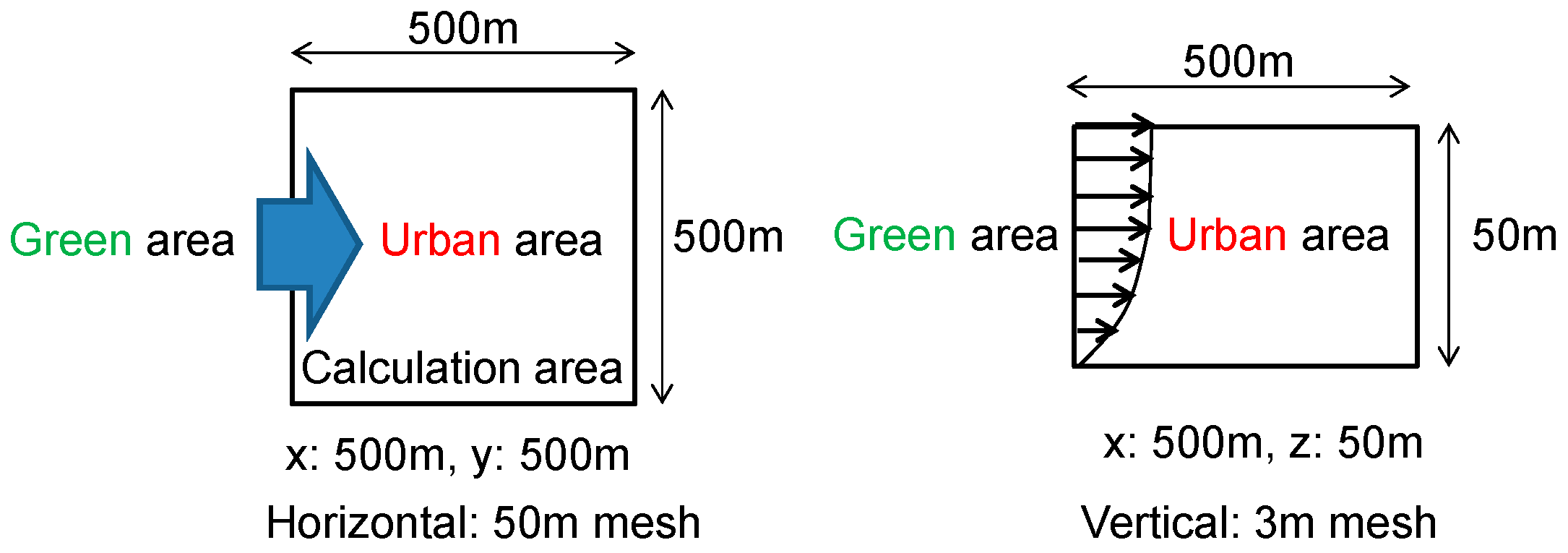
The composition of the model was set according to Moriyama et al. [3], and the calculation conditions were set based on weather conditions at the time of measurement. The mesh size in the horizontal direction was set to 50 m in correspondence with the selection policies of the measurement points. The calculation condition as shown in Figure 4 expresses the phenomenon flowing out from the green area to the urban area in three dimensions. The vertical air temperature profile in the green area was uniformly given for the inflow condition. The upper wind velocity at 50 m high was relatively large, as it was measured under conditions where a sea breeze was dominant.
3.2. Results
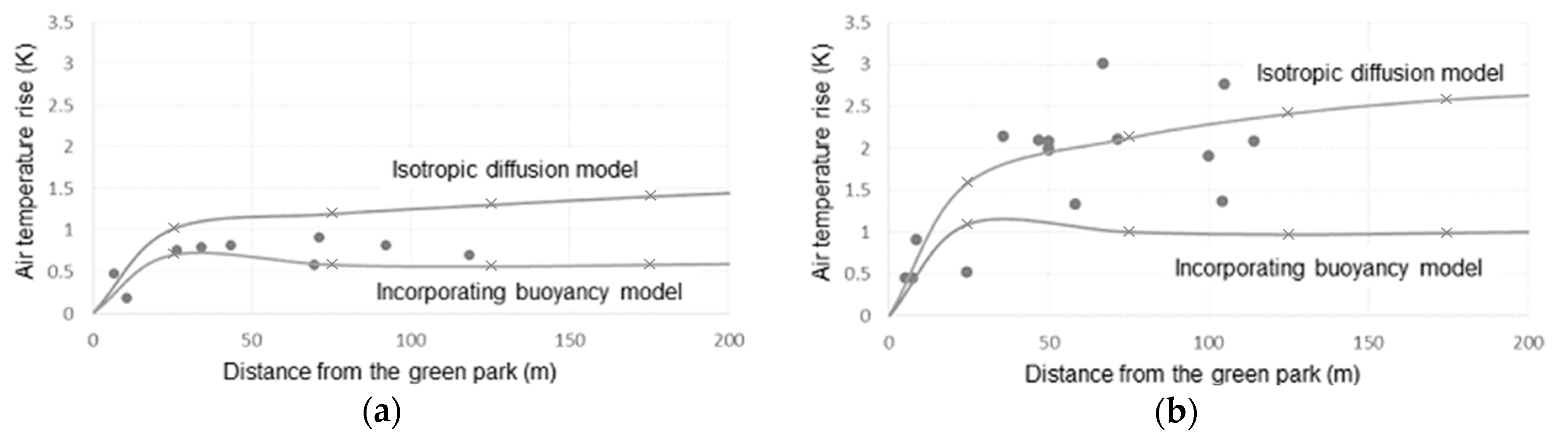
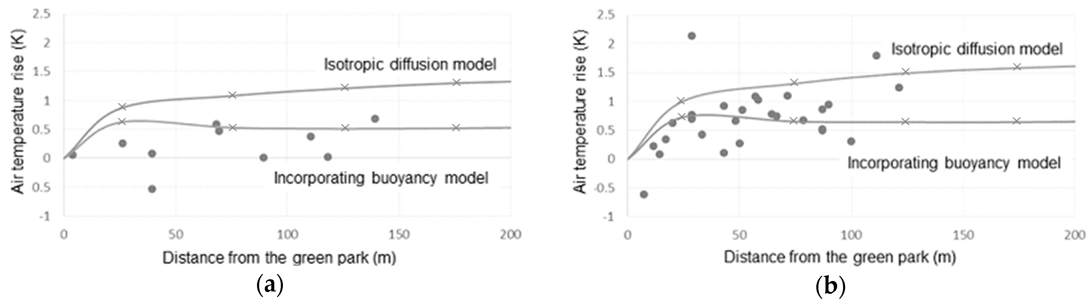
Calculation and measurement results for air temperature rise with distance from the green area are shown in Figure 5 and Figure 6. The results in both isotropic and non-isotropic diffusion models are shown. In the isotropic diffusion model, the horizontal and vertical eddy viscosity coefficients νt are given by Equation (6). In the non-isotropic diffusion model, the eddy viscosity coefficient νt in the vertical direction is given by the formula of Equation (7) when considering the buoyancy effect. Distance from the green area and the heat flux component of the calculation result, at 13:00 in the mesh near the ground surface, is shown in Figure 7. In the incorporated buoyancy model, the sensible heat flux supplied from the ground surface is transported in the vertical direction due to the vertical diffusion effect, so air temperature in the mesh near the ground surface does not rise. The part of the urban area more than 50 m from the green area is dominated by the diffusion effect in the vertical direction over the advection effect.
When the inflow wind velocity is large, the calculation result in the incorporated buoyancy model tends to coincide with the measurement result of the air temperature. When the inflow wind velocity is small, the calculation result in the isotropic diffusion model, in which the diffusion effect in the vertical direction is not prominent, is close to the measurement result of the air temperature.
Therefore, the calculation result by the previous study, using the isotropic diffusion model, may be matched with the measurement result when the inflow wind velocity is small. This is shown in the right-hand panels of Figure 5 and Figure 6. Even if the distance from the green area is 150 m or more, air temperature rises more and its effect may thus extend to over 200 m. Since the inflow wind velocity is small, the vertical diffusion effect is also small, and the air temperature rise in the urban area is thus larger than when the inflow wind velocity is large. At this time air temperature in the urban area varies considerably because of the influence of local ventilation, solar radiation shielding, etc. This can be seen from the measurement results in the right-hand panel of Figure 5.
4. Discussion
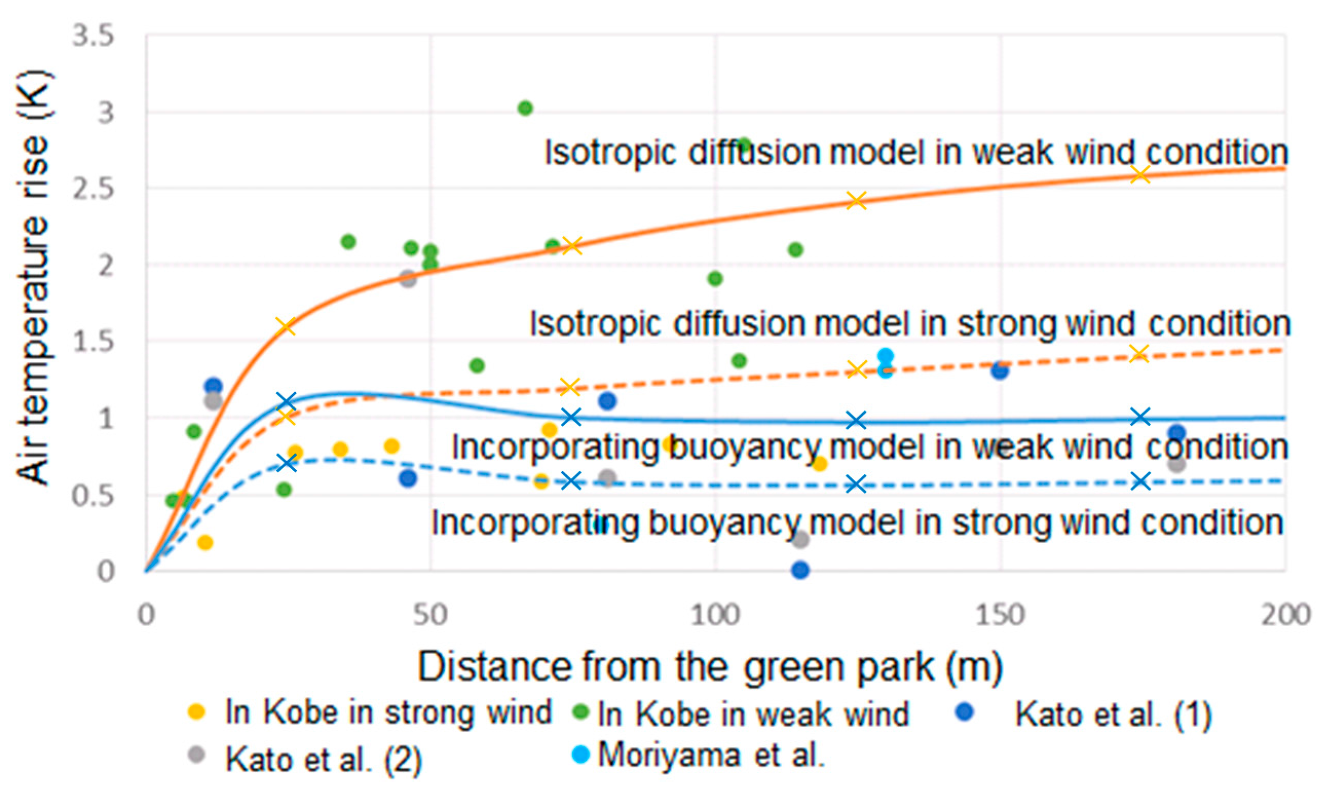
In addition to the measurement results in Kobe City, the calculation results in Figure 8 and Figure 9 were also compared to the measurement results in the urban area around Koishikawa park in Tokyo by Kato et al. [9], and several parks in Osaka city by Moriyama et al. [10]. In the results measured in Tokyo and Osaka, air temperature does not rise as it enters the part of the urban area more than 50 m from the green area. On the other hand, Honjo and Takakura [2] explained that the range of the effects of urban green areas extends to about 100 to 300 m into the surrounding urban area. Since they used the isotropic diffusion model, it is recognized that it was a finding only in the case of weak wind.
In order to discuss this in more detail, a recalculation was carried out, improving the spatial resolution in the urban area near the green area. An outline of the modified calculation conditions is shown in Figure 10. The horizontal mesh size was changed to 5 m from 50 m as in the above calculation. The other calculation conditions were not changed.
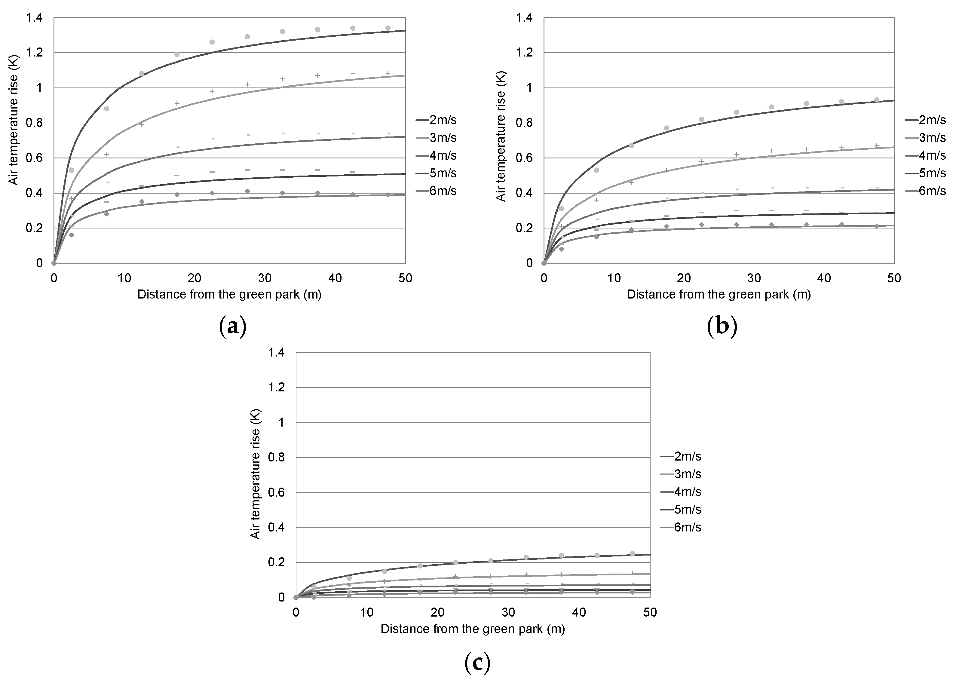
Calculation results of air temperature rise according to the distance from the green area are shown in Figure 11. Sensible heat flux from the ground surface in the urban area was assumed to be 236.7 W/m2 for daytime and 28.3 W/m2 for evening. A value of 132.5 W/m2 was also assumed for their intermediate value. When entering the urban area air temperature rises sharply. The smaller the wind velocity, the larger the distance influenced by the green area, and the larger the air temperature rise. As the distance from the green area increases, air temperature becomes constant. When entering the part of the urban area more than 50 m from the green area, the air temperature near the ground surface is dominated by the diffusion effect in the vertical direction rather than the advection effect from the green area.
In general, air temperature rise ∆T (K) due to the development of the urban boundary layer is expressed by Equation (12).
where k is the ratio of entrainment (0 to 1), H is the sensible heat flux from the ground surface (W/m2), L is the distance from the boundary (m), α is air temperature gradient (K/m), Cp is the specific heat of air (=1000 J/(kgK)), ρ is air density (=1.2 kg/m3), and U is wind velocity (m/s). Assuming α = 0.006 (K/m), it becomes Equation (13).
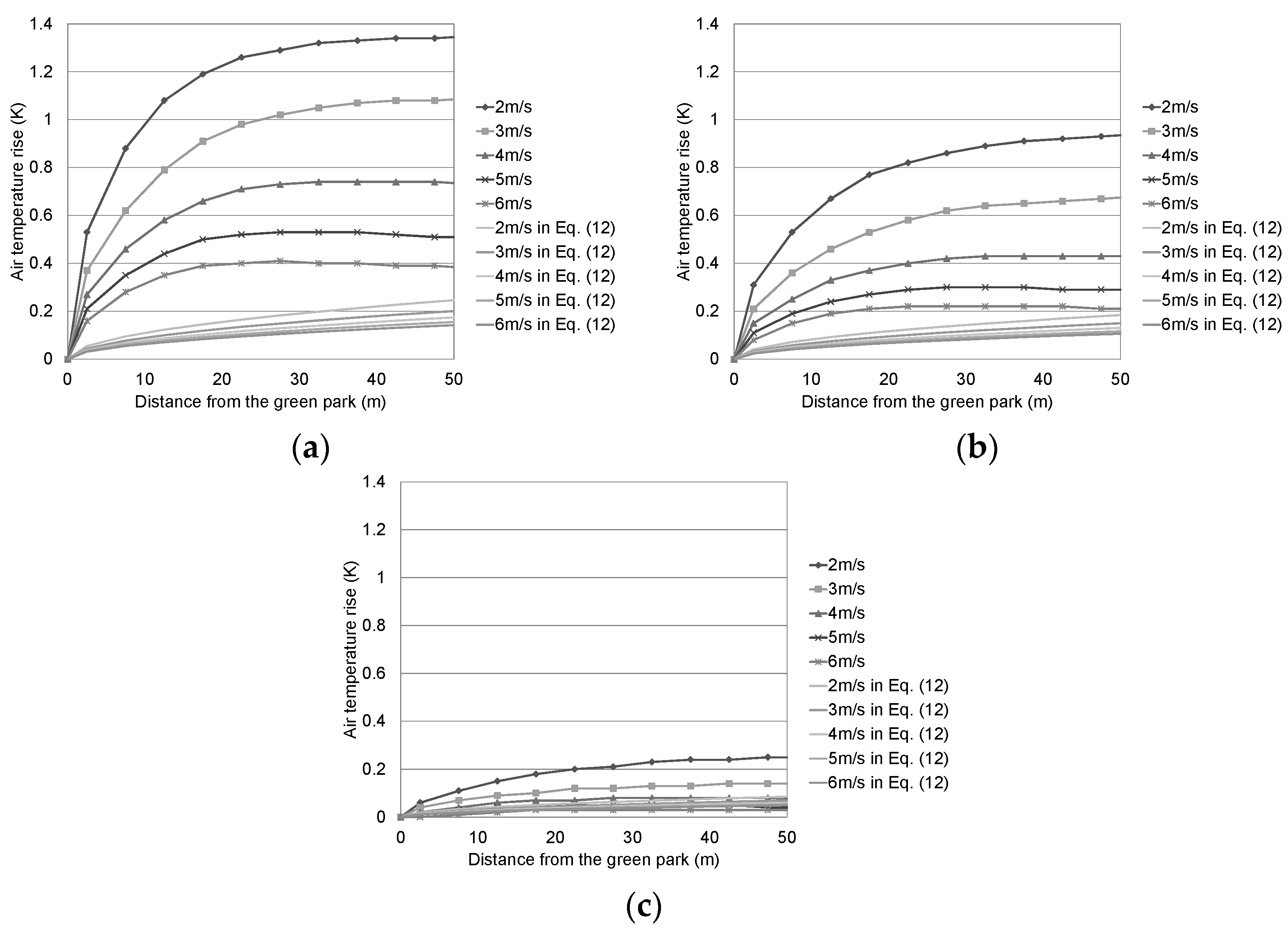
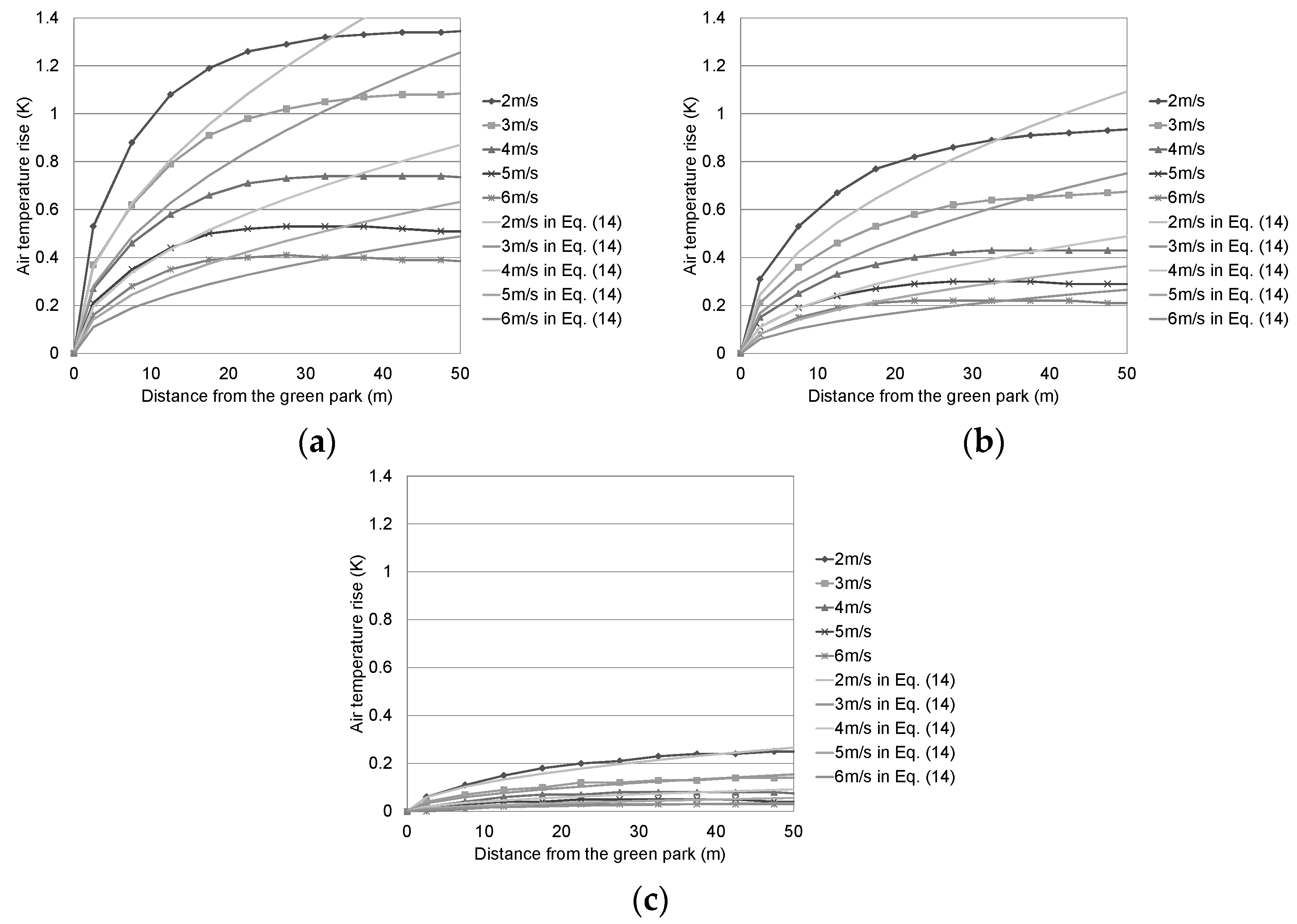
Air temperature rise ∆T, by Equation (12), when k = 0 is shown in Figure 12 together with the calculation results. Equation (12) is calculated using the boundary layer thickness h = ∆T/α. Actually, when the development of the boundary layer is not sufficient and h is small, α should be set to be large. Then, air temperature rise ∆T approximated by Equation (14) is shown in Figure 13. The coefficient a at this time is shown in Table 3. It is larger than the 0.0032 used in Equation (12).
As described above, the calculated air temperature near the ground surface rises sharply as it enters the urban area. This is because of the sensible heat flux from the ground surface, and when entering the area beyond about 50 m, it becomes almost constant. On the other hand, the approximate value of the air temperature due to the development of the boundary layer monotonically rises with the distance from the green area. Therefore, we considered an approximation based on the following equation where air temperature rise becomes constant as the distance goes above a certain value. Air temperature rise ∆T by Equation (15) is shown in Figure 14 together with the calculation results. When entering the urban area, air temperature rises sharply, and when entering the area beyond a certain distance it becomes almost constant.
5. Conclusions
In order to clarify the characteristics of air temperature rise in an urban area on the leeward side of a green area, mobile measurements and calculations expressing advection and diffusion effects are made. These calculations were then verified by comparison with the measurement results. The relationship between the distance from the green area to each mobile measurement point in the urban area and the air temperature rise is analyzed using the measurement results in Kobe city. At a measurement point where the distance from the green area is 30 m or more, the air temperature of the urban area becomes unaffected by the green area.
Calculation results and measurement results for air temperature rise with distance from the green area are compared when an isotropic diffusion model and an incorporated buoyancy model are applied for the vertical diffusion term. From the comparison with the measurement results in Kobe City, as well as in Tokyo and Osaka, it is considered that air temperature does not rise as it enters the part of the urban area beyond more than 50 m from the edge of the green area. The air temperature rise in the urban area near the green area, due to the development of the urban boundary layer, is expressed using the sensible heat flux from the ground surface, the distance from the green area and the wind velocity. We considered an approximation of air temperature rise in order to express the following situation: when entering the urban area, air temperature rises sharply, and when passing beyond a certain distance, it becomes almost constant.
Acknowledgments
I thank the urban planning bureau of Kobe city office for their cooperation with respect to our measurements. I used the modified source code by Moriyama et al. for the calculations.
Conflicts of Interest
The author declares no conflict of interest.
References
- Givoni, B. Impact of planted areas on urban environmental quality: A review. Atmos. Environ. 1991, 25B, 289–299. [Google Scholar] [CrossRef]
- Honjo, T.; Takakura, T. Simulation of thermal effects of urban green areas on their surrounding areas. Energy Build. 1990–1991, 15, 443–446. [Google Scholar] [CrossRef]
- Moriyama, M.; Takebayashi, H.; Fukumoto, K. Effects of Green Areas on Urban Air Temperature by Numerical Solution. Mem. Grad. Sch. Sci. Technol. Kobe Univ. 1997, 15, 101–115. [Google Scholar]
- Bowler, D.E.; Buyung-Ali, L.; Knight, T.M.; Pullin, A.S. Urban greening to cool towns and cities: A systematic review of the empirical evidence. Landsc. Urban Plan. 2010, 97, 147–155. [Google Scholar] [CrossRef]
- Ca, V.T.; Asaeda, T.; Abu, E.M. Reductions in air conditioning energy caused by a nearby park. Energy Build. 1998, 29, 83–92. [Google Scholar] [CrossRef]
- Yu, C.; Hien, W.N. Thermal benefits of city parks. Energy Build. 2006, 38, 105–120. [Google Scholar] [CrossRef]
- Yagi, R.; Takebayashi, H. Study on the near ground surface temperature influenced by surface temperature and wind velocity. Eighth Natl. Conf. Heat Isl. Inst. Int. 2013, 1, 48–49. [Google Scholar]
- Ashie, Y.; Ca, V.T. Developing a three-dimensional urban canopy model by space-averaging method: Development of the urban climate simulation system for urban and architectural planning Part 2. J. Environ. Eng. (Trans. AIJ) 2004, 69, 45–51. [Google Scholar] [CrossRef]
- Kato, T.; Yamada, T.; Hino, M. Spatial structure of air temperature and humidityin urban park forest and its surrounding. J. Inst. Sci. Eng. Chuo Univ. 2016, 12, 63–71. [Google Scholar]
- Moriyama, M.; Kono, H.; Yoshida, A.; Miyazaki, H.; Takebayashi, H. Data analysis on “cool spot” effect of green canopy in urban areas. J. Archit. Plan. (Trans. AIJ) 2001, 66, 49–56. [Google Scholar] [CrossRef]
Figure 1.
Mobile measurement points and aerial photograph, all located in Kobe city, Japan. (a) Higashi-yuen Park and business area; (b) Ishiyagawa Park and residential area; (c) Okurayama Park and residential area.
Figure 1.
Mobile measurement points and aerial photograph, all located in Kobe city, Japan. (a) Higashi-yuen Park and business area; (b) Ishiyagawa Park and residential area; (c) Okurayama Park and residential area.


Figure 2.
Measurement results of air temperature at the fixed measurement points.

Figure 3.
Distance from the green area to each mobile measurement point in urban area and air temperature rise (a) at 13:00; (b) at 17:00.
Figure 3.
Distance from the green area to each mobile measurement point in urban area and air temperature rise (a) at 13:00; (b) at 17:00.

Figure 4.
Outline of calculation conditions.

Figure 5.
Calculation results and measurement results of air temperature rise at 13:00 according to the distance from the green area. (a) strong wind case; (b) weak wind case.
Figure 5.
Calculation results and measurement results of air temperature rise at 13:00 according to the distance from the green area. (a) strong wind case; (b) weak wind case.

Figure 6.
Calculation results and measurement results of air temperature rise at 17:00 according to the distance from the green area. (a) strong wind case; (b) weak wind case.
Figure 6.
Calculation results and measurement results of air temperature rise at 17:00 according to the distance from the green area. (a) strong wind case; (b) weak wind case.

Figure 7.
Distance from the green area and heat flux component of the calculation result at 13:00. (a) isotropic diffusion model; (b) incorporating buoyancy model.
Figure 7.
Distance from the green area and heat flux component of the calculation result at 13:00. (a) isotropic diffusion model; (b) incorporating buoyancy model.
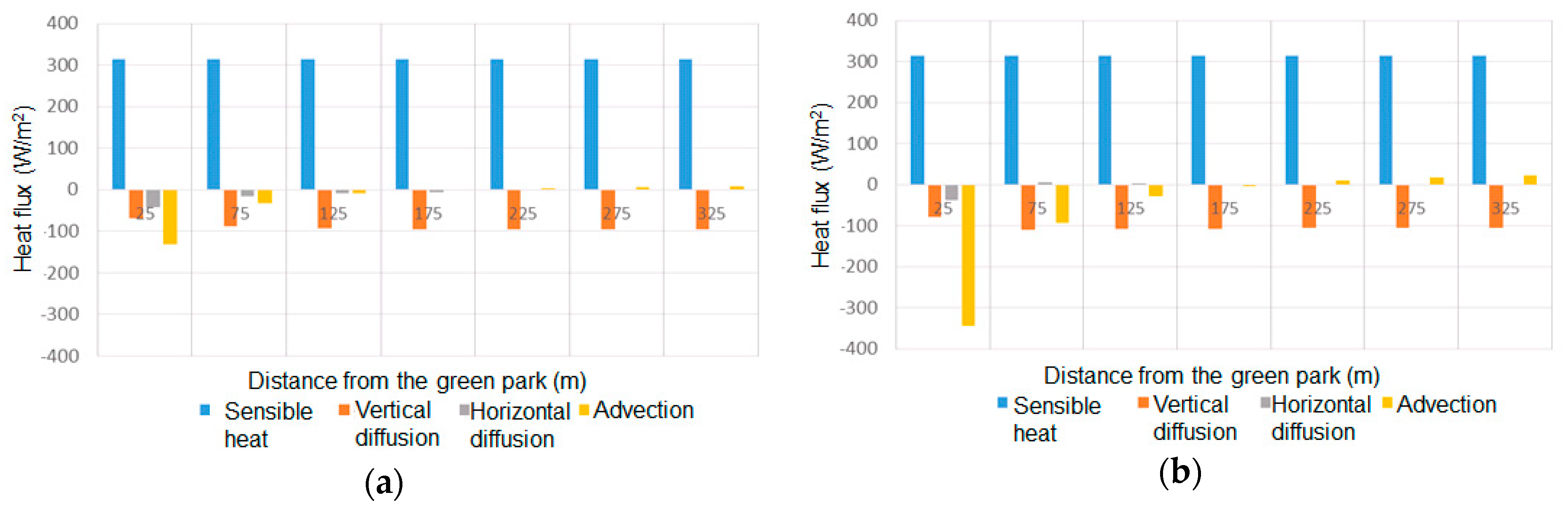
Figure 8.
Distance from the green area and the air temperature rise in several urban areas in the daytime.
Figure 8.
Distance from the green area and the air temperature rise in several urban areas in the daytime.

Figure 9.
Distance from the green area and air temperature rise in several urban areas in the evening.
Figure 9.
Distance from the green area and air temperature rise in several urban areas in the evening.
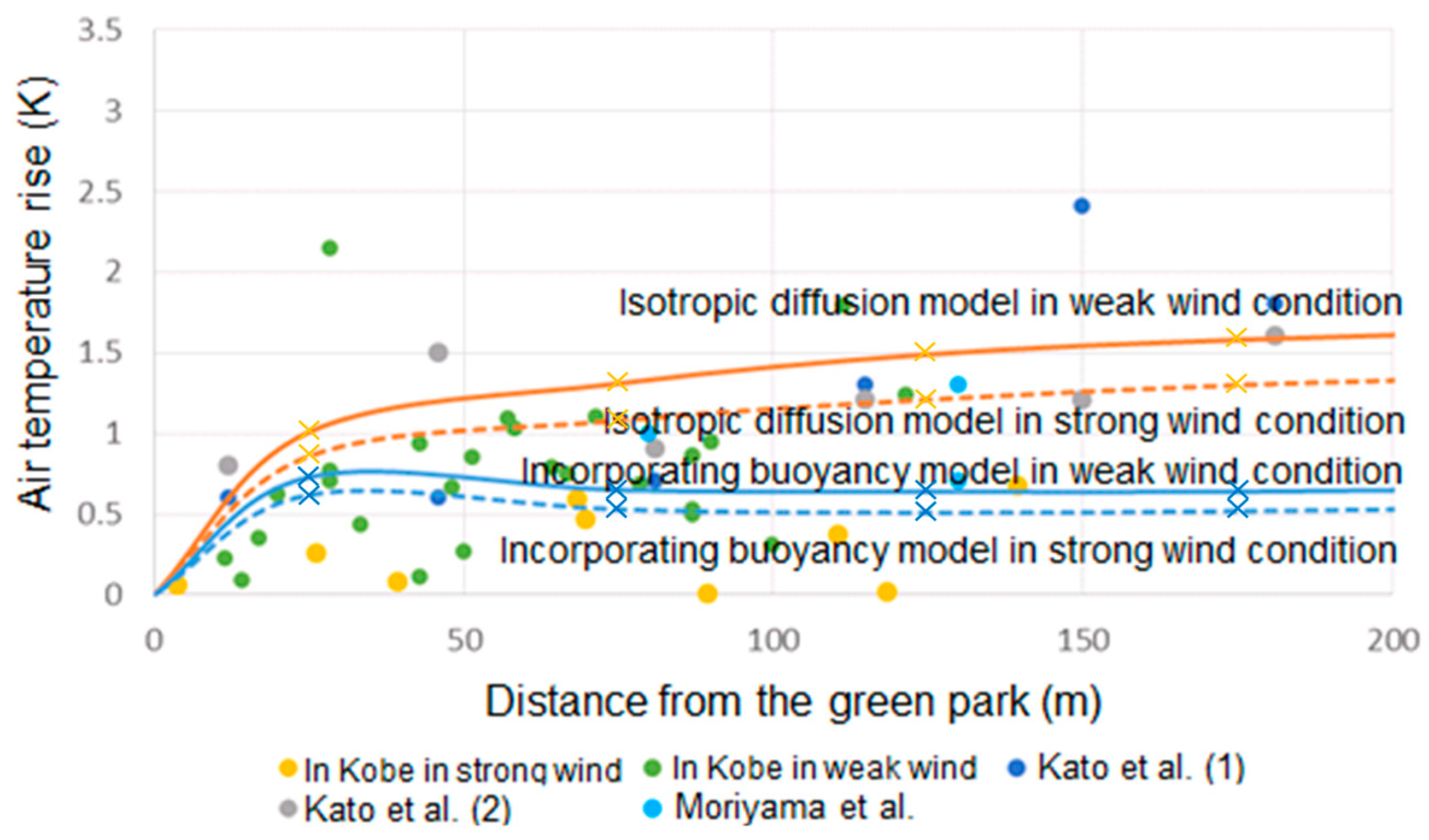
Figure 10.
Outline of modified calculation conditions.
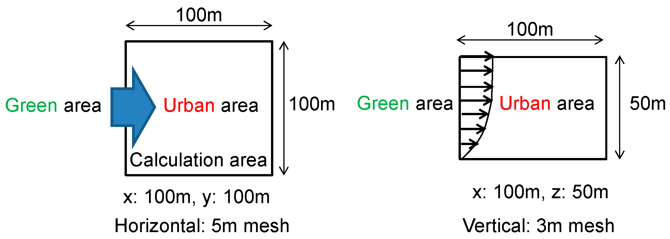
Figure 11.
Calculation results of air temperature rise according to the distance from the green area. In the cases where the sensible heat flux is (a) 236.7 W/m2; (b) 132.5 W/m2; (c) 28.3 W/m2.
Figure 11.
Calculation results of air temperature rise according to the distance from the green area. In the cases where the sensible heat flux is (a) 236.7 W/m2; (b) 132.5 W/m2; (c) 28.3 W/m2.
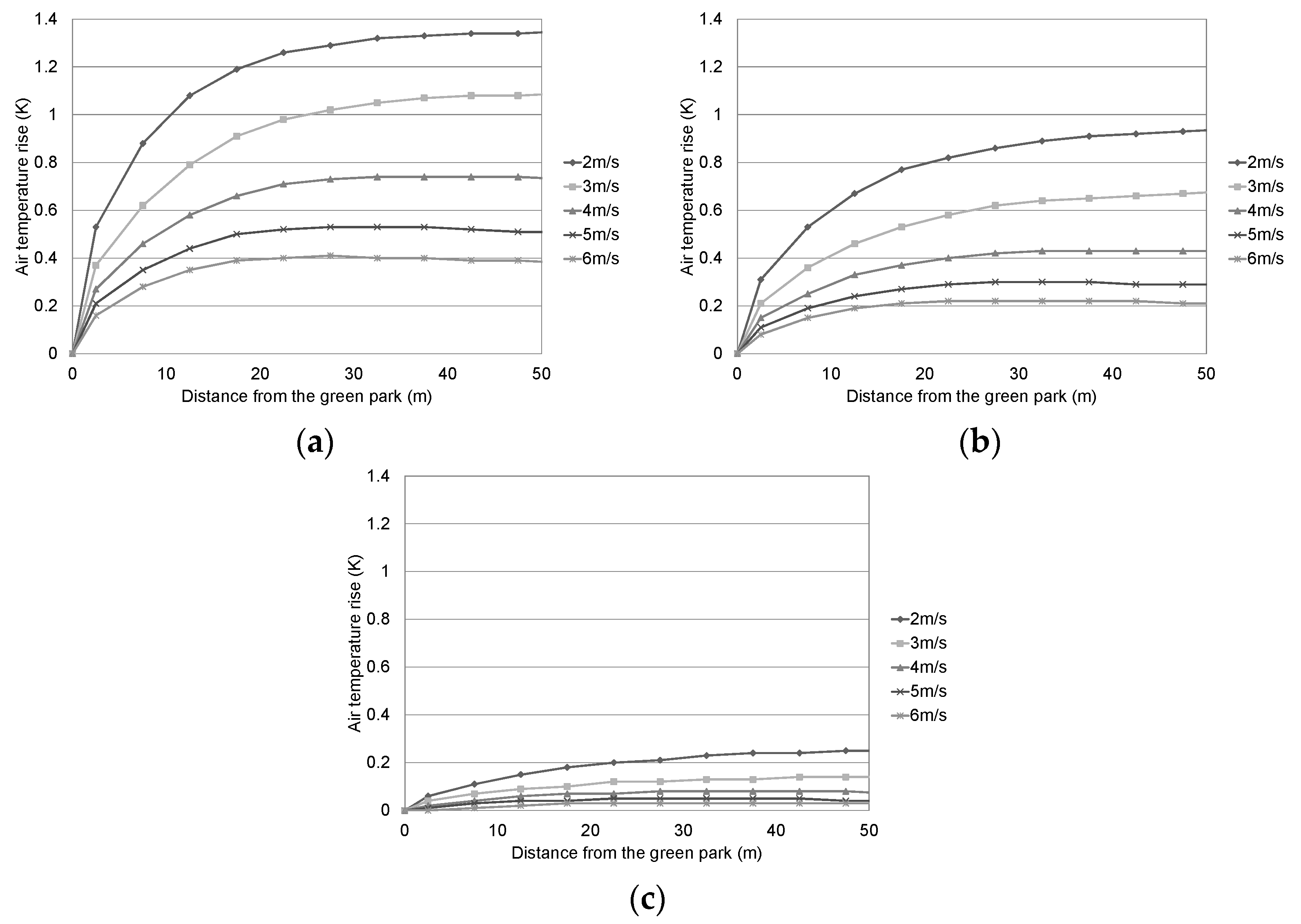
Figure 12.
Air temperature rise by Equation (12). In the cases where the sensible heat flux is (a) 236.7 W/m2; (b) 132.5 W/m2; (c) 28.3 W/m2.
Figure 12.
Air temperature rise by Equation (12). In the cases where the sensible heat flux is (a) 236.7 W/m2; (b) 132.5 W/m2; (c) 28.3 W/m2.

Figure 13.
Air temperature rise by Equation (14). In the cases where the sensible heat flux is (a) 236.7 W/m2; (b) 132.5 W/m2; (c) 28.3 W/m2.
Figure 13.
Air temperature rise by Equation (14). In the cases where the sensible heat flux is (a) 236.7 W/m2; (b) 132.5 W/m2; (c) 28.3 W/m2.

Figure 14.
Air temperature rise by Equation (15). In the cases where the sensible heat flux is (a) 236.7 W/m2; (b) 132.5 W/m2; (c) 28.3 W/m2.
Figure 14.
Air temperature rise by Equation (15). In the cases where the sensible heat flux is (a) 236.7 W/m2; (b) 132.5 W/m2; (c) 28.3 W/m2.

Table 1.
Measuring device and method.
| Device | Method | Accuracy of Device | |
|---|---|---|---|
| Air temperature | Thermistor with solar radiation shield | Averaged for 5 min by sampling every 5 s | ±0.5 K |
| Wind direction | Windsock | Highest frequency in 30 s | by visual inspection |
| Wind velocity | Hot-wire anemometer | Averaged for 30 s by sampling every second | ±2% of indicated value |
| Surface temperature | Infrared thermometer | Measured on ground and wall surface, a representative material surface at each measurement point was measured several times to obtain stable data | ±1.0 K |
Table 2.
Calculation conditions.
| 13:00 | 17:00 | |
|---|---|---|
| Inflow air temperature with uniform vertical profile | 33 °C | 31 °C |
| Inflow wind velocity at 50 m high with logarithmic vertical profile | Large: 5.6 m/s Small: 4.1 m/s | Large: 4.7 m/s Small: 4.2 m/s |
| Sensible heat from ground surface | 314 W/m2 | 196 W/m2 |
| Roughness parameter | 0.5 m | |
| Horizontal mesh size | 50 m | |
| Vertical mesh size | 3 m | |
Table 3.
Coefficient a when it is approximated by Equation (14).
| 2 m/s | 3 m/s | 4 m/s | 5 m/s | 6 m/s | |
|---|---|---|---|---|---|
| 236.7 W/m2 | 0.021 | 0.020 | 0.016 | 0.013 | 0.011 |
| 132.5 W/m2 | 0.019 | 0.016 | 0.012 | 0.010 | 0.008 |
| 28.3 W/m2 | 0.010 | 0.007 | 0.005 | 0.003 | 0.002 |
© 2017 by the author. Licensee MDPI, Basel, Switzerland. This article is an open access article distributed under the terms and conditions of the Creative Commons Attribution (CC BY) license (http://creativecommons.org/licenses/by/4.0/).
Share and Cite
MDPI and ACS Style
Takebayashi, H. Influence of Urban Green Area on Air Temperature of Surrounding Built-Up Area. Climate 2017, 5, 60. https://doi.org/10.3390/cli5030060
AMA Style
Takebayashi H. Influence of Urban Green Area on Air Temperature of Surrounding Built-Up Area. Climate. 2017; 5(3):60. https://doi.org/10.3390/cli5030060
Chicago/Turabian StyleTakebayashi, Hideki. 2017. "Influence of Urban Green Area on Air Temperature of Surrounding Built-Up Area" Climate 5, no. 3: 60. https://doi.org/10.3390/cli5030060
Note that from the first issue of 2016, this journal uses article numbers instead of page numbers. See further details here.