Towards Dependence of Tropical Cyclone Intensity on Sea Surface Temperature and Its Response in a Warming World

Abstract

Tropical Cyclone (TC) systems affect global ocean heat transport due to mixing of the upper ocean and impact climate dynamics. A higher Sea Surface Temperature (SST), other influencing factors remaining supportive, fuels TC genesis and intensification. The atmospheric thermodynamic profile, especially the sea-air temperature contrast (SAT), also contributes due to heat transfer and affects TC’s maximum surface wind speed (V_max) explained by enthalpy exchange processes. Studies have shown that SST can approximately be used as a proxy for SAT. As a part of an ongoing effort in this work, we simplistically explored the connection between SST and V_max from a climatological perspective. Subsequently, estimated V_max is applied to compute Power Dissipation Index (an upper limit on TC’s destructive potential). The model is developed using long-term observational SST reconstructions employed on three independent SST datasets and validated against an established model. This simple approach excluded physical parameters, such as mixing ratio and atmospheric profile, however, renders it generally suitable to compute potential intensity associated with TCs spatially and weakly temporally and performs well for stronger storms. A futuristic prediction by the HadCM3 climate model under doubled CO₂ indicates stronger storm surface wind speeds and rising SST, especially in the Northern Hemisphere.

1. Introduction

In recent years there has been a growing interest in understanding the response of tropical cyclone (TC) activity to climate change [1,2,3]. Most work on TC involves its track prediction that primarily needs knowledge of large-scale environmental circulation, available for most of the tropics. However, TC intensity (TCI) determination requires consideration of fine sub-grid scale processes and hence poses a challenge to the scientific community. The theoretical upper bound on a TC’s intensity is termed as its Potential Intensity (PI) which can be calculated using Sea Surface Temperature (SST), Sea Level Pressure (SLP) and profiles of atmospheric temperature and mixing ratio [1,2].

There are three major techniques developed to date to explore this subject (cf., [4]). Most of the published works on the subject mention examining the intensity, based on atmospheric thermodynamics and equations governing atmospheric flows in association with TC [5,6,7,8]. Another approach to determine cyclone intensity is based on a time-dependent numerical modeling technique. This method considers a weak TC seeded into a known environment. The model is then integrated with the progressing time until the cyclone’s maximum intensity is accomplished [9,10]. A third technique makes use of observational data to statistically find TC intensity as a function of observed oceanic-atmospheric variables, such as SST [11,12,13]. For example, a previous study using ~45 year statistical regressions has shown that SST has a dominating influence in high hurricane seasons, independent of all known other factors and that sea warming explained 61% ± 34% of the anomalous Atlantic hurricane activity in 1995 to 95% [14].

All approaches have their relative merits for the intended applications and their potential areas of improvements. Generally speaking, evolved models using thermodynamic equations (physical models) are expected to yield better characterization of tropical cyclones (e.g., [5,6,7,8]), however, if these models consider cyclones to be in isolation, then the effects of the environment will be ignored. Also, they require a range of accurate input parameters that may not always be precisely available. Numerical models also require multiple parameters but most users likely use the default values (however, exact initial values are desirable) and the model must inherently be accurately parameterized. The use of observational data is based on statistical relationships (stochastic models), which certainly has the advantage of ease-of-use when data is available but may yield results which are grossly over- or under- estimated and will be precise only for those points where the condition matches with the input to the regression model. It is understandably insufficient to attempt to characterize TC with a simple set of coefficients, however, they are still effective as long as the retrieval errors are in a permissible range. This third methodology is extended in this work and its results are compared with those of a physical model. The assumption, therefore, is that SST is one of the main driving forces for TC intensification.

Hazard mitigation planning and management requires a good estimate of tropical cyclone intensity and their identification, in a prompt and timely manner. As stated earlier, the genesis of thunderstorms, its intensification and conversion to cyclonic systems and dissipation is a synergistic process and depends on a number of physical parameters, such as SST, sea-air temperature contrast (SAT), SLP and mixing ratio. This paper documents the first step of an ongoing investigation where we simplistically explored the connection between SST (as the source of energy to fuel a TC system and as a proxy for SAT) and TC’s maximum surface wind speed (V_max) using climatological data (not instantaneous). The aim is to see if this simplistic approach captures the major part of the variability of the maximum wind speed, as compared to a more evolved model. Provided that such simplistic approaches match developed methods at the least initially, another goal is to provide a simple empirical relation to determine cyclone intensity using statistical analysis, which incorporates sensitivity of storm strength on the ocean temperature. In future studies of this ongoing effort, we will extend our model to capture the remaining inconsistencies by including more model variables, keeping in mind the ease of application as a key requirement. Another focus of this study is to estimate changes in tropical cyclone intensity patterns in the warming world, including under a doubled CO₂ scenario, using a model simulation.

The paper is organized as follows: Section 2 briefly describes the theoretical background. The methods employed and datasets used are given in Section 3. Section 4 comprises the major results and discussions concerning: (a) development of a linear model for maximum achievable cyclone winds (V_max); (b) the relation between SST and sustained wind speed and understanding its role through enthalpy and spatial distribution of V_max; (c) application of linear model outputs to the HadCM3 Model. Temporal analyses using wavelet spectrum and time series plots are given in Section 5. Section 6 summarizes the paper and gives a future outlook.

2. Theoretical Background

The total power dissipation of a TC is proportional to the cube of its wind speeds [3,6,15,16]. The Potential Intensity (PI) of a TC can be expressed in terms of the surface drag coefficient, the surface air density and the magnitude of the surface winds, integrated over a TC’s radius ([3,6]). Historical data does not provide information of a storm’s dimension and therefore it is difficult to use historical datasets in order to determine their PI. Further studies shed light on the radial wind contours [17] and characterization of storm’s dimension [18] and the drag coefficient [19]. With this background and further simplifications, the Power Dissipation Index (PDI) of a TC is given by [3]:

$$PDI=\underset{0}{\overset{\tau }{{\displaystyle \int }}}{V}_{\text{max}}^{3}dt$$

(1)

Here, V_max represents the maximum sustained wind speeds at 10 meters above the surface. A TC’s PDI is a better indicator of a storm’s threat than a cyclone’s frequency or its intensity alone [3]. PDI is also of interest in reference to its influence on thermohaline circulation [20] and upper ocean mixing [3]. Owing to the simplicity of practically implementing Equation (1) and its relevance to define destructiveness in association with a tropical cyclone, we have made use of this index instead of more traditional indices, such as the hurricane severity index [21], the cyclone intensity scale [22] and the accumulated cyclone energy index [23], all of which require a range of input parameters.

It is also well known that SST plays a vital role in cyclone genesis and intensification [20,24]. SST in its own may not always be sufficient to fully determine TC intensification. For instance, the Atlantic storm Earl in 1992 attained a maximum speed of 28 m/s at an SST of about 27 °C, while the Atlantic hurricane Bonnie, during the same season, gained a maximum speed of 49 m/s with an ocean temperature of about 25 °C [11]. However, SST is a critical parameter necessary to fuel intensification of thunderstorms that may or may not grow into a cyclone, depending on other parameters. In this study we present an empirical model to estimate cyclone intensity using SST.

3. Methods Employed and Datasets Used

3.1. Methodology

The local SST tends to influence the atmospheric state above it and affects the Potential Intensity of a cyclone [2,25,26]. Temperature anomalies of the troposphere also depend upon variation in tropical SST [27].

Three datasets have been used in our study for formulation and verification purposes [28,29,30,31]; one for model formulation and the other two for independent dataset verification. The first part of this work makes use of observation-based reanalysis of datasets, ERSST.V3b [30], for constructing a simple statistical model to determine (tropical and) local maximum sustained wind speeds, V_max, from (tropical and) regional SSTs. The output of Emanuel’s model (with ERSST.V3b) provides TC potential intensity measured in terms of V_max and P_min, and provides input V_max to the regression model. This simple model is then tested on two additional and independent SST input datasets, Optimally Interpolated SST (OISST.V2) [29] and COBE [31], ranging from 1800 [30] and 1891 [31] onwards, making the model suitable for computing the cyclone’s strength and also for retrospective studies during the pre-satellite era. For purposes of comparison and validation, our model outputs are then compared against those of an established model [5] that is also implemented in this work (Section 3.1.1). The second part of this work focuses on exploring temporal and spatial variation of V_max derived using the relationship built in the first part. After understanding how V_max values change over time, in the remaining part of this work we also explore how it responds to a warmer world with doubled CO₂. The outcome of the HadCM3 climate model is employed for this purpose.

Our simple approach, which holds only for a climatological snapshot of average values (not necessarily for instantaneous values), is based on two assumptions. First, TC’s maximum surface wind speed V_max values and sea-air temperature contrast (SAT) show a distinct correlation in their variabilities (cf., [32]). Second, SST and air temperature values are linearly related to a first order approximation [33,34] and thus SST and SAT (SST minus air temperature) too are correlated. Based on these assumptions, we developed a linear relationship between SST and V_max whose reliability is tested further using two long-term SST reanalysis datasets. A test of hypothesis was further applied to estimate the strength of this correlation.

3.1.1. Computation of Sustained Wind Speeds

Sustained wind speeds, V_max, are derived using monthly SST (averaged over 792 months from 1948 to 2014), sounding data, sea level pressure and specific humidity from reanalysis datasets as input to the algorithm available at ftp://texmex.mit.edu/pub/emanuel/TCMAX/pcmin_2013.f [5]. In this work, we first calculate V_max using the established model referenced above, using 3 different SST datasets. This algorithm also requires additional parameters (see Section 3.2.1). Then we define V_maxNew as TC’s sustained wind speeds computed using only SST as input to our model, as explained later in Section 4. The results of these two methods are statistically compared, showing a reasonable agreement (see Section 4.1).

3.1.2. Warmer World Scenario with Increased CO₂

In order to explore changes in SST and TCI when the CO₂ is doubled in the Earth’s climate system, a suite of coupled oceanic-atmospheric models was employed. The model runs to get SST are obtained from the HadCM3 based on present day CO₂ levels and then in a doubled CO₂ scenario. We use Ensemble Perturbed Physics Ensembles (PPE) by estimating the mean response of 53 different model versions with changes in physical parameters involved in the model.

There are two primary reasons for exploiting the PPE technique here. The first reason is the capability of the method to sample mean climate states in relatively broad bounds [35]. Secondly, a wide range of climate forcing and feedback are efficiently handled under increased levels of greenhouse gases (like CO₂). The demand for better computation of uncertainties in climate forecast estimates gave rise to the Perturbed Physics Technique [36]. In this approach, we consider a single model structure and perturb the magnitudes of uncertain variables within an allowed range. The range is decided with the help of the people involved in parameterization development and by rigorous inspection of the modeling literature. Experimental runs with single models can then be developed in “ensemble mode”, depending upon the availability of computation power and time.

Considering a changed climate situation of doubled CO₂, SST values thus obtained from the model runs are then plugged into our statistical model to obtain V_maxNew for the case. Then newly obtained V_maxNew values over a grid in the tropics for the present day and the climate change scenario are subtracted to determine the net change in V_max.

3.2. Data Used

3.2.1. Reanalysis Data

A monthly mean reanalysis dataset provided by the National Centers for Environmental Prediction (NCEP)/National Center for Atmospheric Research (NCAR) is used as input to determine tropical cyclone strength using an algorithm based on the thermodynamic model for cyclone intensity. The algorithm [15] takes SST, SLP, atmospheric temperature and mixing ratio as input variables and yields maximum achievable cyclone winds (V_max) and theoretically minimum attainable TC pressure (P_min). Unlike SST [29,30,31] and SLP [37,38] which are considered at surface level, atmospheric temperature and mixing ratio are considered in the vertical atmosphere. Atmospheric soundings are available up to the lower stratosphere for 16 pressure levels (plus the surface): 1000, 925, 850, 700, 600, 500, 400, 300, 200, 150, 100, 70, 50, 30, 20 and 10 mb. SLP, atmospheric soundings and mixing ratio datasets, used in developing the statistical model, are considered from 1948 onwards. (SST is expressed in °C, SLP in mb, atmospheric temperature in °C and the mixing ratio in g/kg.) The value of the mixing ratio ranges between 0 g/kg for cold continents to 20 g/kg for warm tropical areas.

Three climatological SSTs are used here. The first set of SST data, ERSST.V3b [30], is the National Oceanic and Atmospheric Administration (NOAA) extended reconstruction made using the most recently available Comprehensive Ocean-Atmosphere Data Sets (COADS) and improved, statistical methods that allow stable re-constructions using sparse data. (ERSST.V3b is an improved, extended reconstruction over the second version.) The second set of SST dataset, COBE SST [31], is a monthly mean of global fields created during June, 2011 at NOAA’s Physical Sciences Division (PSD) of the Earth System Research Laboratory (ESRL) using the gridded data from the Japanese Reanalysis Project (JRA). The third SST dataset employed is NOAA’s second version optimum interpolation OISST.V2 [29]. These optimally interpolated blended data are an in situ and satellite SST combined analysis for climate [28]. The satellite SSTs ingested are the Advanced Very High Resolution Radiometer (AVHRR) infrared retrievals onboard NOAA -11 through -19 polar-orbiters, with only one platform used at a time and the data are anchored to in situ drifters (approximating a bulk depth of ~20 cm). It is worth mentioning that in recent years, a substantial effort has been invested to generate blended satellite SSTs from multiple platforms, many of which also ingest in situ data in their optimal interpolation scheme [39,40]. We have chosen OISST.V2 because of its extended range going back in time. The datasets, other than SST used here, were available at 2.5° × 2.5° (144 × 73 cells, globally), OISST.V2 and COBE SST at 1° × 1° and ERSST.V3b at 2° × 2° grids. These datasets were aggregated to a common grid of 1° × 1° employing bilinear interpolation for analyses.

3.2.2. Climate Model Data

In order to explore the influence of projected change of SST on cyclone intensity with enhanced levels of green house gases, we make use of climate model ensembles as derived from the third version of UK Met Office Hadley Centre Climate Model, HadCM3 [41]. Considered climate model ensembles taken from the physics ensemble are retrieved from HadCM3.

HadCM3 is a coupled ocean-atmospheric general circulation model developed at the Hadley Centre, UK and is one of the primary models used for IPCC third assessment report (2001) [42]. The model possesses a high resolution over the oceans and thus does not require flux correction (artificial heat and fresh water fluxes over the ocean floor) [43]. The model has a grid resolution of 3.75° × 2.5° (longitude × latitude; Arakawa-B type grid), which corresponds to approximately 300 km spacing between the points and is comparable to T42 truncation in a particular spectral model. The model has a time step of 30 min which includes sub-time steps, per time step of half an hour.

4. Results and Discussion

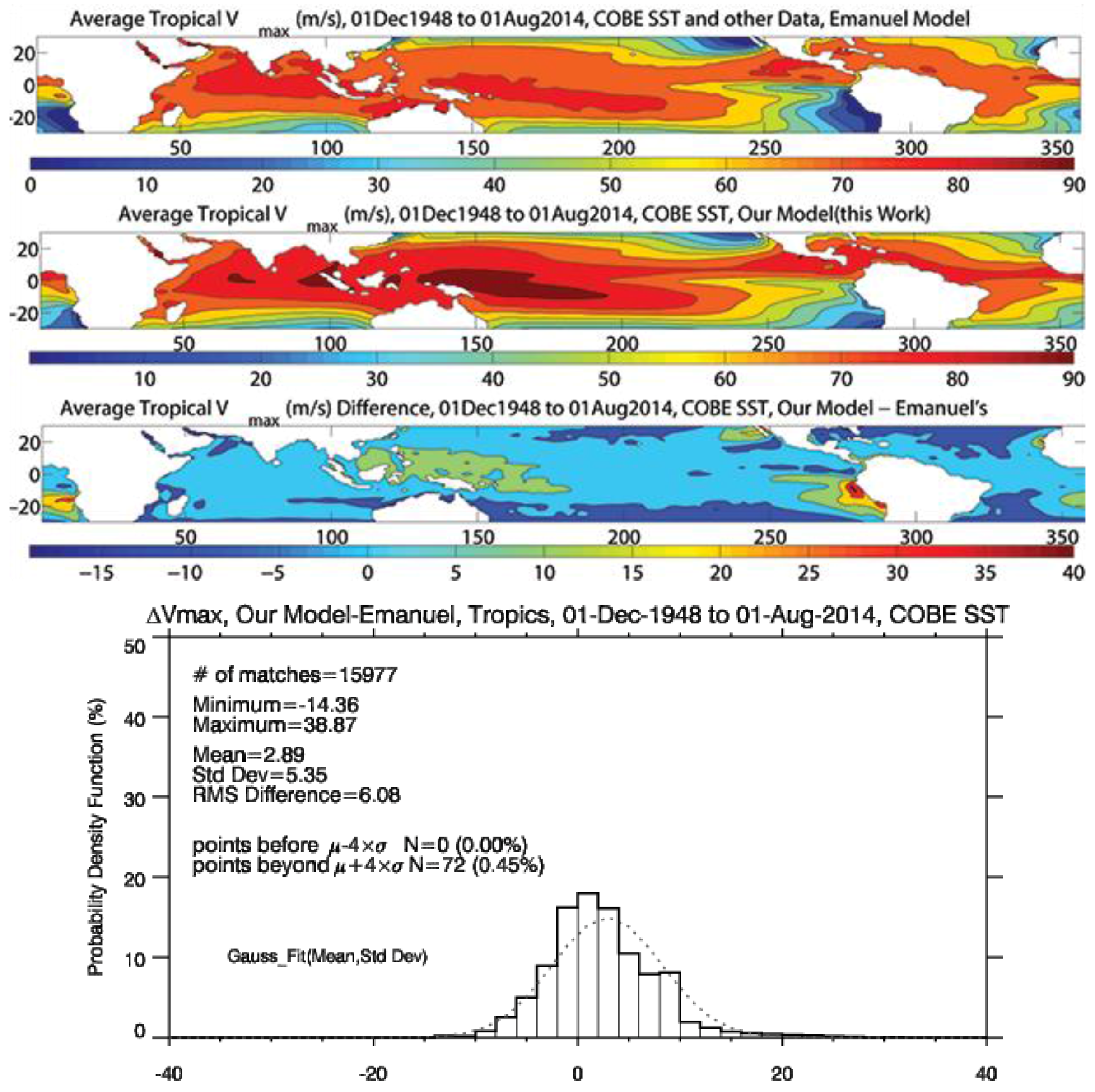
4.1. Development of a Linear V_max Model and Its Validation against an Established Model

The assumptions behind our approach to formulate a simplistic approach to compute V_max only from cyclone-prone SST values and regions are two-fold: (a) TC’s V_max values and sea-air temperature contrast (SAT) are correlated; (b) SST and air temperature (AT) values are approximately related, therefore are sea-air temperature contrast and SST. On the first assumption, the time-evolution of V_max and SAT has been shown to be identical in their directions (not amplitude) during phases of intense storms (cf., [32]) due to enhanced vertical transport. (An offline analysis also showed significant spatial linear correlation with sea-air temperature contrast.). Secondly, mean AT calculated employing the mean value theorem, cf., equation A18 in [33], has been subsequently shown to be related to surface temperature (T_s) in a linear way. Various researchers have used this formulation, where the form of the equation remains the same but the coefficients vary depending on the area of their study. For example, AT = 55.8 + 0.77 × T_s is reported in ([34], also see Figure 3 therein) for their study area. We have not used these values but made the assumption that SAT and SST are correlated with a scatter permissible for our purposes and developed a linear relationship between SST and V_max, whose reliability is tested further using two independent inputs.

Based on the above assumptions that V_max and SST for cyclone-prone conditions (all SST values in the tropics) are correlated, at least to a first order approximation, we have performed a linear regression (r² = 0.95) for the averaged datasets described in Section 3.1.1. Subsequently, the model is applied for climatological averaged values and with a time series analysis also performed in Section 5. Here, we denote our modeled V_max as V_maxNew.

$${\mathrm{V}}_{\text{maxNew}}=6.3\times \text{SST}-102$$

(2)

V_maxNew, as obtained from our statistical model (Equation 2), also shows a significantly high correlation with that of V_max obtained from Emanuel’s model (r² = 0.95). In order to validate these modeled TC wind speeds, both against an established method [15] and across different SST inputs, we calculate both V_max and V_maxNew for each of the three SST data as inputs. Results using COBE [29,30,31] are shown in Figure 1 (COBE SST is independent of the input used for determining the model parameters) and using ERSST.V3b and OISST.V2 are supplementary, shown in Figures S1 and S2, respectively. We acknowledge that this simplistic linear model can be improved by including more parameters to reduce the scatter, however as we show here, this model works well for V_max in the tropics, especially for the higher values. In addition, our goal is to be able to use and provide other users with a simple, easy-to-use model based on parameters that are readily available and in a timely manner. Figure 1 provides a visual comparison of V_max from two different outputs, from Emanuel’s model and from our simplistic model, using COBE SST as input.

The structural resemblance between Figure 1 (row 1) and Figure 1 (row 2) implies that V_maxNew is capable of capturing most of the V_max structures in the tropics, which is encouraging given our simplistic approach. However on an average, our model shows somewhat higher V_max values of 2.89 m/s mean difference as seen in Figure 1 (row 4). These ‘higher differences’ are relatively evenly distributed to a smaller magnitude throughout the tropics and distinctly off the coasts of Angola, Namibia, Senegal and Peru to higher magnitudes. These higher values are seen on the histogram in Figure 1 (row 4) as ~0.45% points beyond “Mean ± 4 × Std Dev”.

Supplementary figures show analyses as in Figure 1 but using ERSST.V3b (Figure S1) and OISST.V2 (Figure S2) as SST inputs. For Emanuel’s model, additional data for other required parameters have been used. The results of Figures S1 and S2 are consistent with the results observed from Figure 1, with a slight change of statistical parameters and hence are excluded from re-discussion for brevity.

High correlations between SST and V_max simulations for the three datasets (as mentioned later in this section) correspond to a linear relation between the two variables, thus simplifying the calculation of PDI, at least to a first order approximation. As shown in

Table 1. Summary and intercomparison of tropical cyclone wind speed obtained from Emanuel’s model and our approach with only SST as input. Comparisons are performed for three different SST inputs: COBE, ERSST.V3b and OISST.V2. Other parameters (SLP, specific humidity, atmospheric temperature profile) required for implementing Emanuel’s model are from NCEP reanalysis datasets.

Vmax (m/s)	Emanuel Implementation (Vmax)	Our Model (VmaxNew)	VmaxNew − Vmax (Validation by Comparison)
COBE SST input
Minimum	0.24	0.70	−14.36
Maximum	94.90	92.24	38.87
Mean	66.60	69.07	2.89
Standard Deviation	16.51	16.86	5.35
RMS Difference	-not applicable (n/a)-	-n/a-	6.08
ERSST.V3b input
Minimum	0.24	5.64	−9.84
Maximum	92.81	91.87	35.96
Mean	65.99	68.79	2.98
Standard Deviation	16.80	16.98	5.09
RMS Difference	-n/a-	-n/a-	5.90
OISST.V2 input
Minimum	0.76	0.14	−14.18
Maximum	99.08	93.72	39.61
Mean	66.35	70.08	4.13
Standard Deviation	16.45	16.93	5.40
RMS Difference	-n/a-	-n/a-	6.80

, this simplistic approach yields results approximately similar to those from the more elaborate approach that, however, requires a range of inputs. It is also important to mention here that this approach is valid only for time-integrated, low-spatial resolution datasets (e.g., monthly mean averages at 1° × 1° latitude-longitude grids) and for SST conditions potentially suitable for TC genesis (SSTs>25 °C). By no means, however, does it imply that this relationship between SST and V_max will hold globally for all SST values and in short time-scales (for example on a daily scale and in daytime low wind-speed conditions with reduced mechanical mixing, warming will be higher.) Put differently, on short time scales and high spatial resolutions, SST only cannot predict instantaneous 10 m maximum wind-speeds.

The minor dissimilarities across outputs of various SST inputs, e.g., OISST.V2 and COBE can be further attributed to minor variations in the distribution of SST across the datasets. Discrepancy between the considered SST products can be attributed to difference in the statistical reconstructions used to find SST values in the regions where data was not available. A second reason could be in association with the techniques applied in collecting various SST datasets, for instance, going from the “Bucket” to the “Hull” method. In the Bucket approach, SST is considered to be the water temperature of buckets of water taken from oceans. In the “hulls of ships” method, SST is measured using sensors placed at the hull of a ship. The data products use both in situ and satellite data to obtain SST covering all the ocean basins on earth. (Note that the cause of differences in SST is not the focus of this study; readers are referred to [28,29,30,31,39,40] for more information on blended analysis SST fields.)

We have also studied the effect of differences between various SST analysis fields on the model output (figures not shown for brevity). For example, SAT and SST as obtained from [37] and COBE SST respectively, show significant correlation (r² = 0.98) and so do SAT and V_max (r² = 0.93). These strong connections are then verified using the bootstrapping method [44]. Modeled TC wind speeds, V_maxNew, is appreciably connected with a linear correlation of r² = 0.90 to the storm winds V_max, as computed from reanalysis datasets using ERSST.V3b (figures not shown). Another set of SST values (OISST.V2) employed to compute V_maxNew also give high correlation with V_max (r² = 0.89). These results thus validate our statistical model and further support it. The statistical significance of these correlations was further confirmed by using null hypothesis where p is a matrix of p-values to test the hypothesis of no correlation. In our case, the p-value was found to be close to zero, implying that the correlation is significant.

Since reliable atmospheric temperature profiles before the satellite-era at remote regions are unavailable, we make use of a relationship between PDI and SST which can be used to determine cyclone power in remote regions. It is known [3] that maximum TC wind speed is better correlated with ocean-atmosphere temperature difference than with SST. That is, though warmer SSTs contribute towards a highly supportive environment for TC strengthening, its formation and intensification are strongly influenced by the contrast between ocean temperature and the vertical thermodynamic profile of the atmosphere above it. However, this result suggests that when vertical moisture content and SLP are not available, SST values alone can be used by simply employing the linear regression model suggested here, to approximate TC wind speeds, V_maxNew, and hence the intensity of a cyclone as reflected by the PDI.

4.2. Understanding the Role of Sustained Wind Speed through Enthalpy

This result showing indirect association between SST and sustained wind speed can be explained by considering the contribution of enthalpy exchange between the ocean and the air above during cyclone genesis. A tropical cyclone draws heat energy from the warm ocean water and uses it to evolve and move across the underlying surface against friction. Thus, a TC system can be regarded as a heat engine. At equilibrium, the input energy is equal to the energy going out of the system or is used in a mechanical motion against the surface friction. Using simplifications as described by previous work (cf., [5]) and considering the bulk aerodynamic formula for evaporation [45] and further simplifications as shown earlier in [5], the rate of total energy generated per unit surface area is given by:

$$W_{in}=\epsilon \times Q_{in}=\frac{T_s- T_0}{T_s}\left(C_k\times \rho \times v\times ∆k+C_d\times \rho \times v^3\right)$$

(3)

where, T_s and T₀ refer to temperature at the surface of the ocean (SST) and the atmosphere above it (AT) respectively; C_k represents the enthalpy exchange coefficient; ρ denotes the density of near surface air in kg/m³; v represents wind speeds close to the ground in m/s; ∆k is the difference of enthalpy from the sea surface and the air above it and C_d is the surface drag coefficient.

Equation (3) provides a sound thermodynamic approximation of the behavior of SST and the atmospheric temperature profile during TC genesis in relation to changes in enthalpy (∆k), though deriving this equation involves various assumptions and hence has its own limitations.

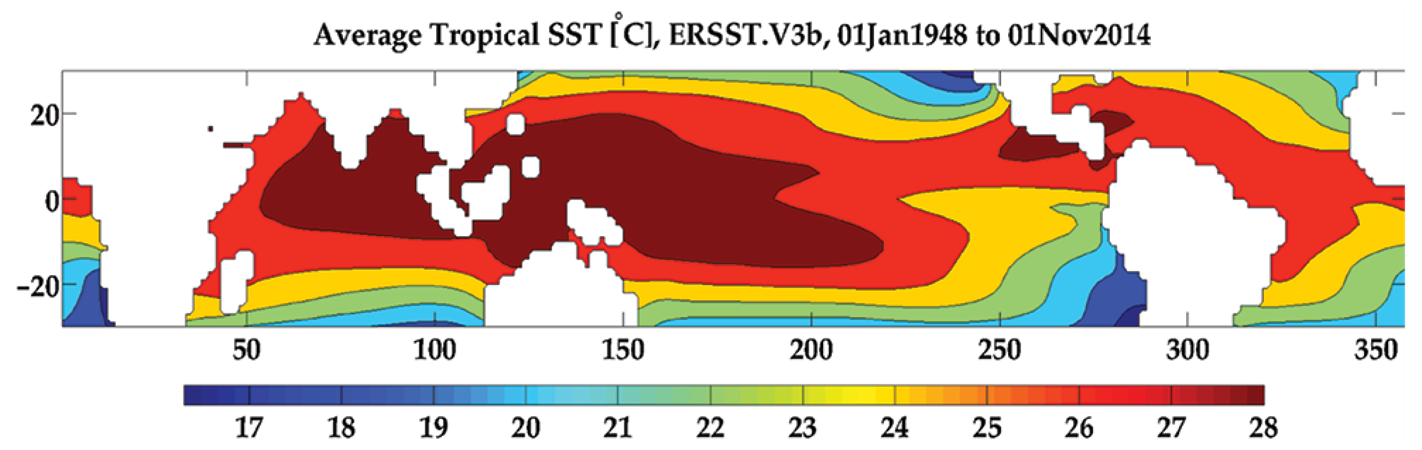
4.3. Spatial Distribution of SST and Comparison with that of V_max

It is observed in Figure 2 that higher temperatures responsible for tropical cyclone intensification are prevalently present along the equator and primarily accumulated in the Northern Hemisphere. In general, the Northern Hemisphere warms more than the Southern Hemisphere, mostly due to more landmass and less ocean surface in the north and the fact that sea-water heats up relatively slowly.

Owing to a wider area occupied by the Pacific Ocean and warmer SSTs in the Pacific in comparison to other oceans, a higher amount of heat energy is available to an evolving TC. However, vertical atmospheric sounding also contributes to cyclogenesis (Section 4.1). SST and theoretically maximum sustained winds speeds, V_max, show roughly similar structures (cf., Figure 1 and Figure 2).

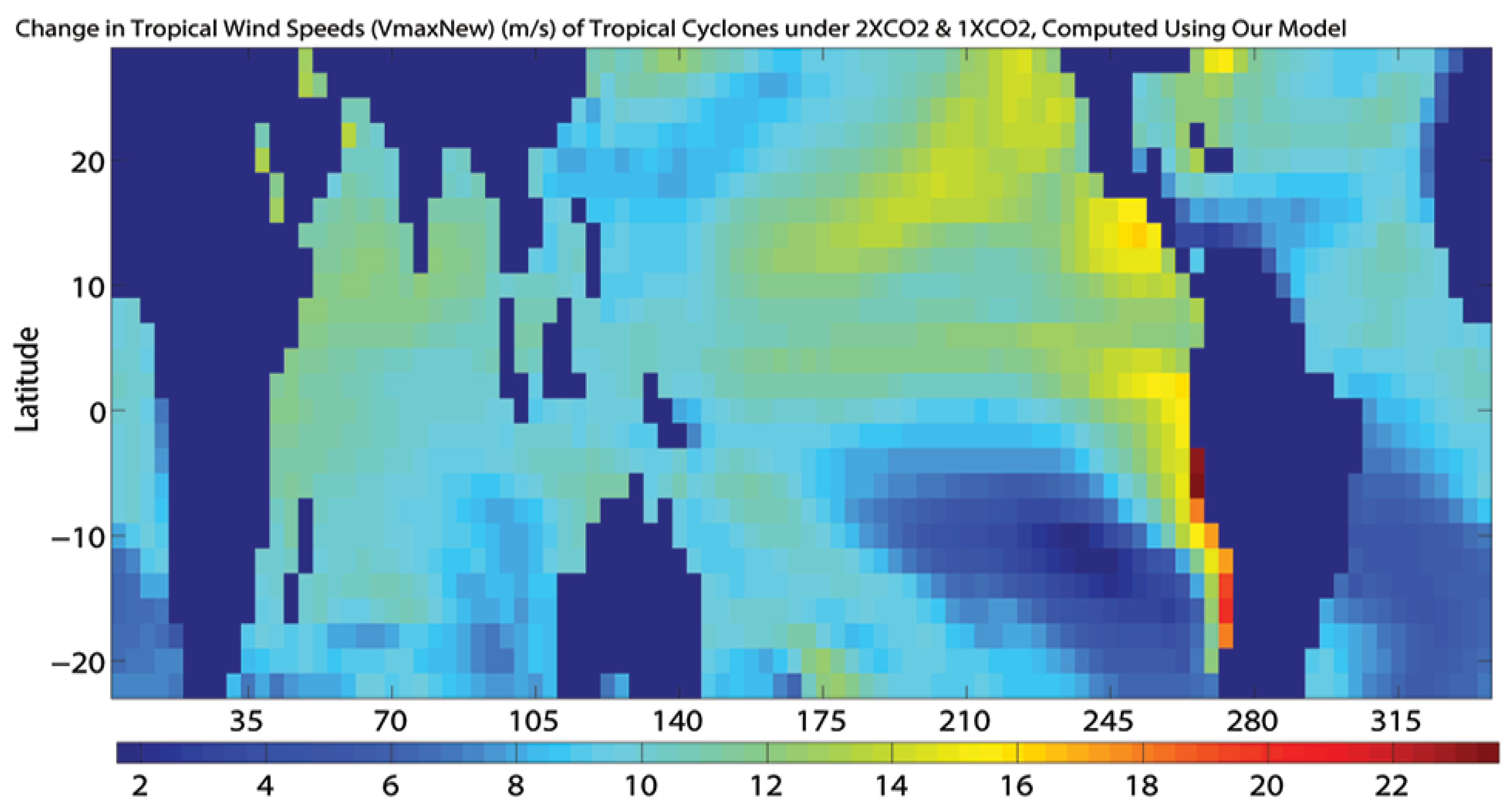
4.4. Application of Linear Model Outputs to HadCM3 Model

We examined changes in SST and hence V_maxNew and PDI projected from the third version of the Hadley Centre Climate Model, HadCM3, where coupled oceanic-atmospheric model outputs were considered in the present day and for a doubled CO₂ scenario. We further applied the resulting ensemble outputs generated by perturbed physics outcomes from the HadCM3 climate model to our statistical model of determining TC winds. This was done to investigate the change in maximum sustained winds and hence cyclone strength ($V_{\text{max}}^3$) when CO₂ levels are doubled in our atmosphere.

It should be noted that the climate model outputs used here are inefficient at resolving the details of tropical cyclone intensity. Both reanalysis and model projections of cyclone wind speeds are found to be highly correlated to SAT, which is in turn are strongly linked to SST. Modeled V_maxNew derived from SST again show high correlation between the reanalysis and HadCM3 model outputs for present day CO₂ level. Using estimated values of SST from the climate model outputs employing both present day and doubled CO₂ cases in our statistical model (Equation (2)), we computed V_maxNew for the two cases mentioned before. The difference in the wind speeds obtained with enhanced CO₂ levels show a significant increase in the maximum sustained winds as shown in Figure 3 and hence cyclone strength. This can be interpreted as stronger storms in the warming world with higher levels of CO₂. Increase in maximum sustained wind speeds is heterogeneous in both hemispheres, with higher increases in the Northern Hemisphere.

The Northeast Pacific shows the highest rise in storm winds [35]. The North Atlantic Ocean comes next in the list of regions. The Indian Ocean followed by the West Pacific region show little influence due to increased levels of CO₂. This change is reversed in the Southern Hemisphere with the West Pacific and Indian Oceans representing regions most prone to destruction by TCs. However, possibly significant statistical differences of the maximum wind speed under a double CO₂ climate appear in the Southeast Pacific. To summarize, it is some sort of dipole effect with regions in the North showing the highest increase, reflecting the lowest increase in the South.

Using Equation (2), we temporally determined a proxy index for V_max, the V_maxNew and then computed the same parameter (V_maxNew) from temporal reanalysis outputs. The linear correlation between the two time series comes out to be only 0.86 in the tropical Atlantic Ocean and about 0.74 in tropical parts of the West Pacific Ocean. Thus, we cannot efficiently employ the spatially derived V_max model to determine the parameter varying temporally. This could be due to the non-stationary behavior of maximum sustained winds. However, as we showed earlier the spatially derived proxy index (V_maxNew), averaged over time, successfully determines maximum sustained wind speeds in the tropics and the cyclone prone ocean basins.

It should be noted that TCs rarely occur within 5° of the Equator due to the negligible value of planetary angular momentum [46]. However, TC wind speed V_max, derived using [1,15] as shown in Figure 1 does show high values due to the absence of this concept in the model and has been excluded from interpretation, although shown on the plot for contouring purposes.

5. Model Application on Temporal Resolution

In order to analyze if this simplistic approach holds adequately in the temporal domain, a time series analysis is performed using wavelet spectrum and standard time series plots. The conclusion that is drawn on spatial domain that this approach holds is also verified for longer time series, implying that the simplistic approach may be used as a fallback for TC studies when reliable atmospheric temperature profiles before the satellite-era, at remote regions, are unavailable for evolved models.

As a first step, we have used wavelet analyses on our output using ERSST.V3.b, individually for all the basins that provided us with the frequency of the V_maxNew signals and their associated time-periods. The major known trends were found to be identified from this simplistic approach, which is encouraging. Whereas the outputs of wavelet spectrum analysis show the frequency vs. time pattern of V_maxNew, it does not provide a clear picture of the temporal behavior. Therefore, as a second step, time series variation of V_maxNew is shown for the corresponding basins.

5.1. Patterns in the V_maxNew

Continuous wavelet power spectra for V_maxNew in different basins are plotted here for further analyses. The black contours on Figure 4, Figure 5, Figure 6, Figure 7 and Figure 8 represent the 5% significance level against the red noise and the cone of influence demarcates the region where edge effects come into effect.

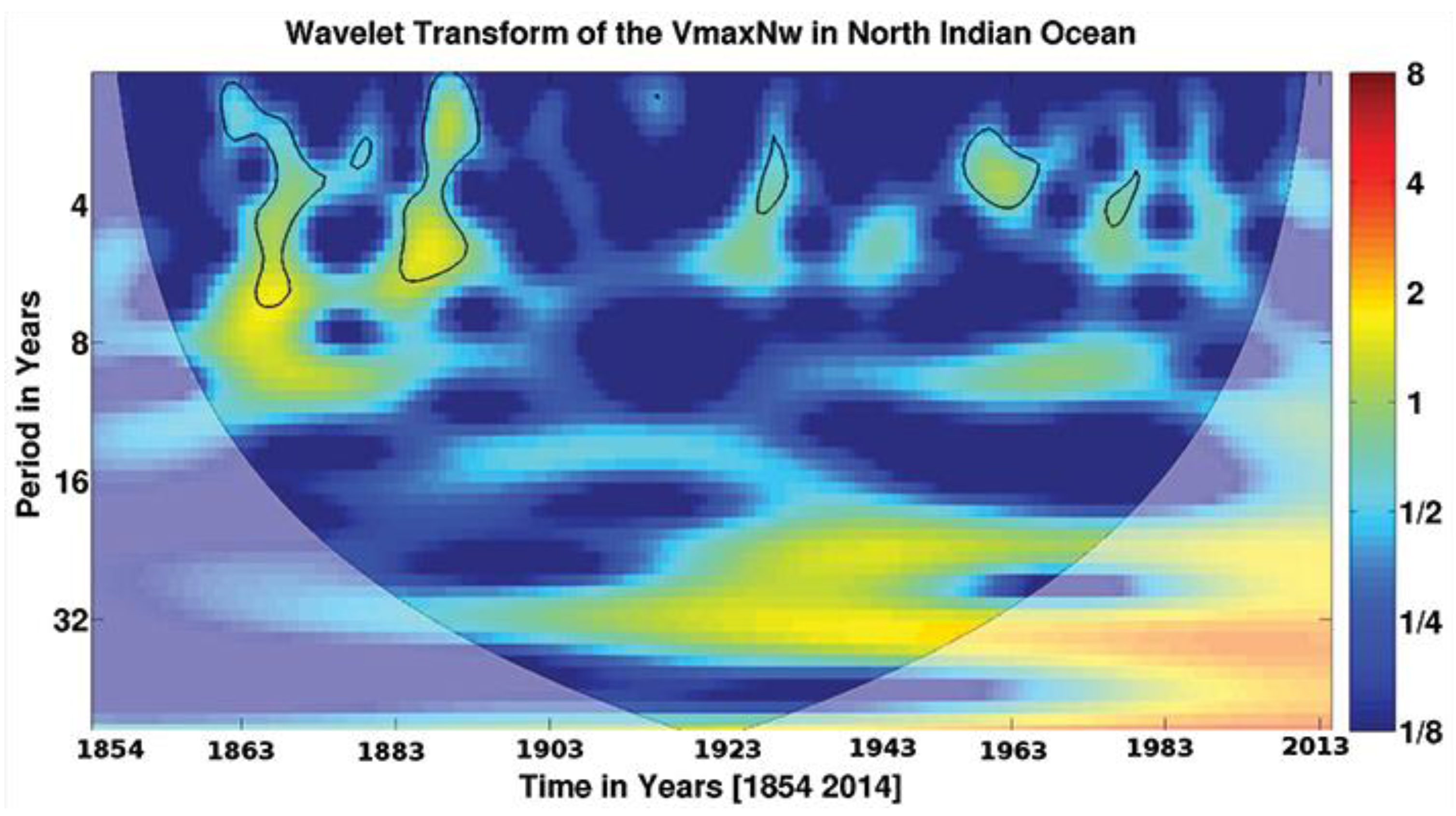
5.1.1. North Indian Ocean

Figure 4 plots the power spectrum in the North Indian Ocean that shows high power in ~6 year band during 1877 and a 5-year cycle in 1901. The two elongated bands (contoured in black) range between ~2–6 years. After these two bands, we can observe a lull period and then a cycle between 3–4 years during 1943, followed by a similar significant cycle around 1984 and again during 1988. All these bands show highest power around 5 years and 3 years that may be associated with the El Niño–Southern Oscillation (ENSO) in the Northwest Pacific and dormant Indian Ocean Dipole cycle respectively.

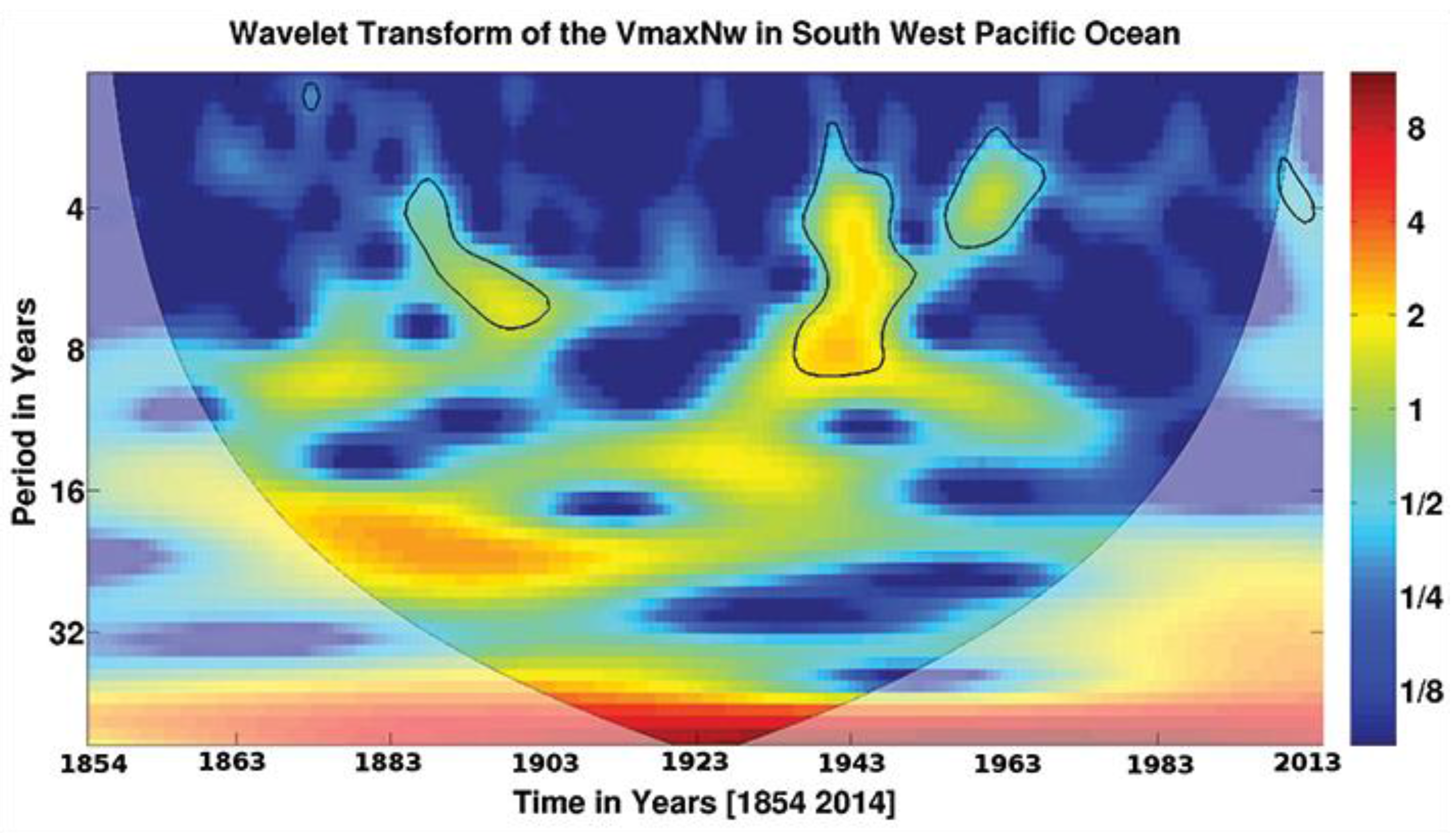
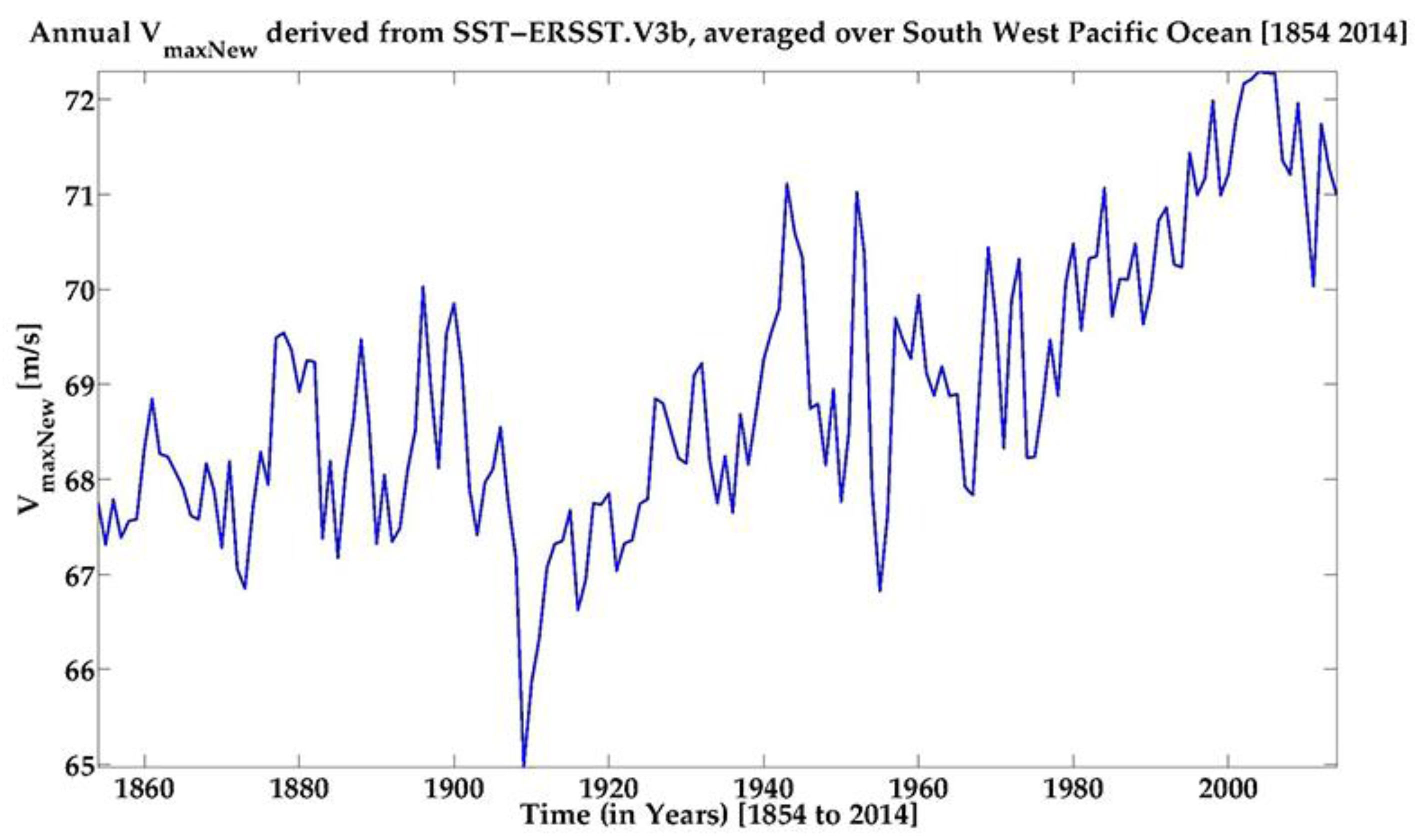
5.1.2. Southwest Pacific Ocean

The continuous wavelet transform of V_maxNew in the Southwest Pacific is shown in Figure 5. Cyclic patterns in the wavelet power are clearly observed in the V_maxNew series. A significant peak in the 2–9 years cycle is apparent around 1954. This cycle of ~9 years may coincide with the Pacific Decadal Oscillations (PDO) which spans 8–12 years period. About a 4 year cycle is also seen around 1972. Another significant cycle possesses a period of 3–7 years during 1910. These oscillations may coincide with the ENSO cycle of 3–7 years (needs further investigation).

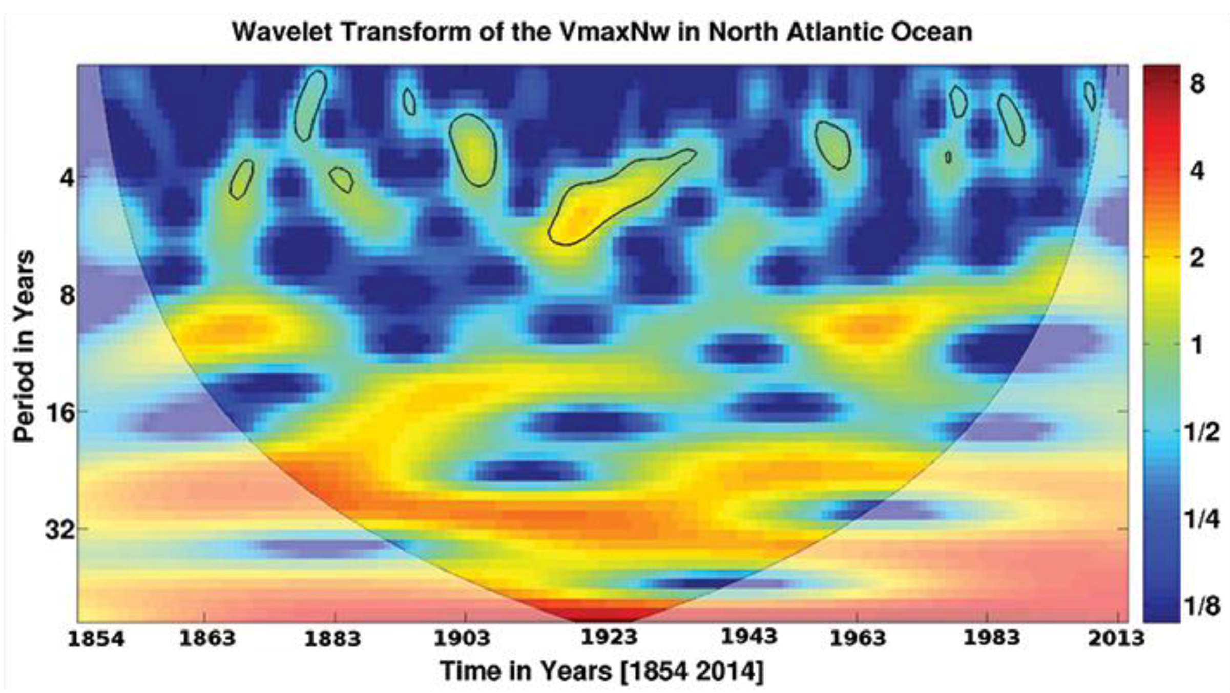
5.1.3. North Atlantic Ocean

The continuous wavelet power spectrum in the North Atlantic is illustrated in Figure 6. A significant peak in the 5 years band around 1934 is apparent. The wavelet spectrum also shows high power with the periodicity of 2–3 years which is widespread and show significant but intermittent occurrences at a difference of about 8–10 years.

5.1.4. Northwest Pacific

Figure 7 presents the continuous wavelet power spectrum of V_maxNew in the Northwest Pacific which shows a significant cycle of ~8 years around 1950 and may be related to the Pacific Decadal Oscillations (PDO) that show up around 1916. Cycles of 2–3 years are widespread during the considered period of 161 years from 1854 to 2014.

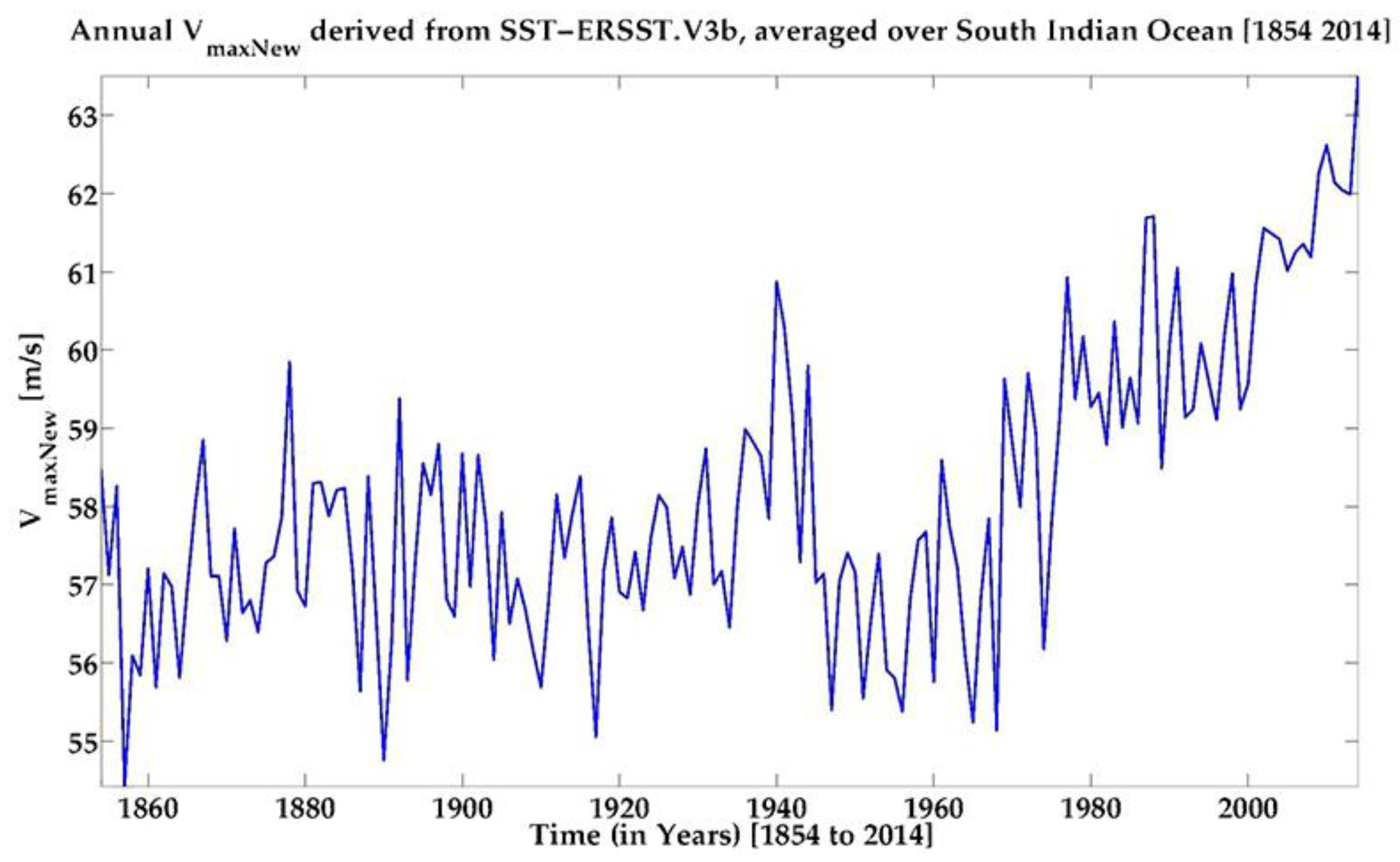
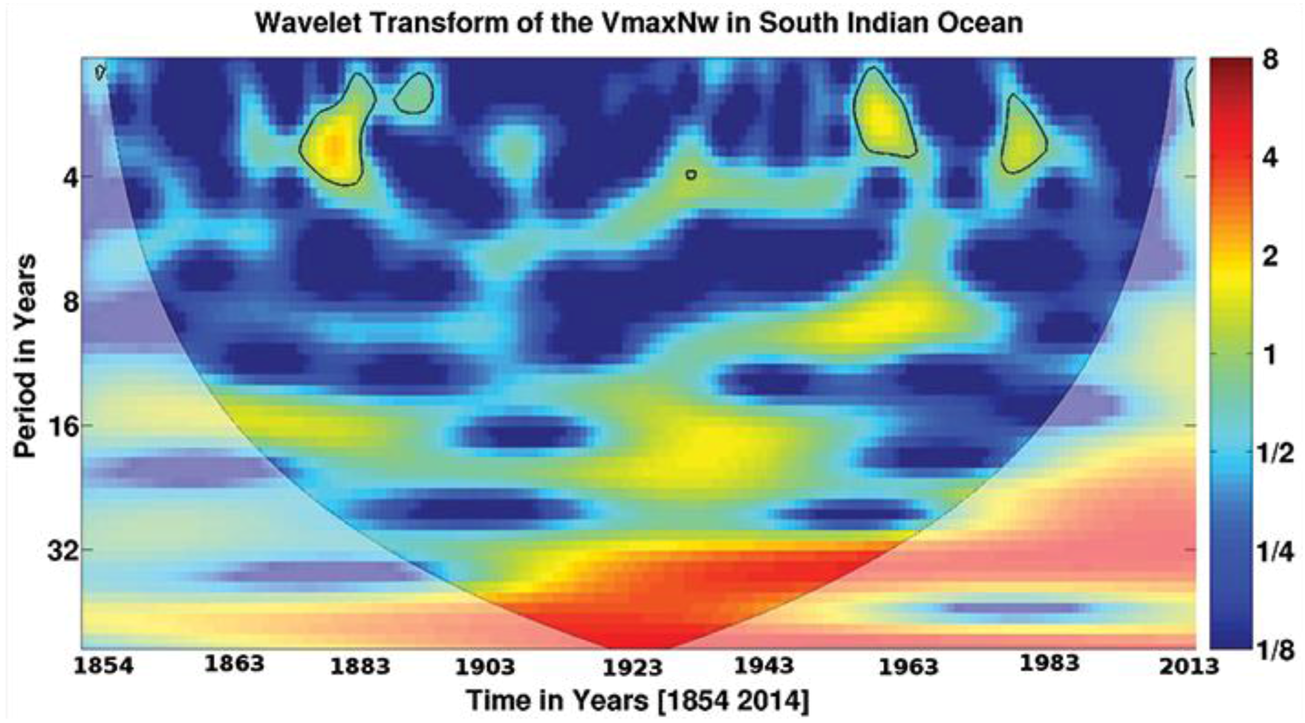
5.1.5. Southern Indian Ocean

Figure 8 exhibits the continuous wavelet power spectrum of V_maxNew in the South Indian Ocean. The figure suggests the occurrence of very few cycles. Most of the power of the signal appears to be concentrated at longer duration cycles (at the bottom of the cone, which however, are not discussed here and detailed analysis is suggested for this region. The most dominant cycle is of ~3 years which occurs around 1991, 1971 and 1891.

It should be noted that the findings from this part of the study shows various significant cycles in the considered ocean basins that may be associated with ENSO, PDO, North Atlantic Oscillation and IOD, as inferred in the description above. However, more detailed analysis is recommended in each of the ocean basins in relation with such natural cycles.

5.2. Time Series Trends

(1)

The Southwest Pacific: Simulated TC wind speed V_maxNew reveals a steep increase since 1910 until 2014 in the Southwest Pacific (Figure 9). A period of 161 years between 1854 to 2014 shows steady fluctuations between 67 to 70 m/s wind speed.

(2)

The South Indian Ocean: Trends in V_maxNew in the South Indian Ocean (Figure 10) show a lull period between 1854 and 1940 followed by a year of sharp rise and then fall. V_maxNew since 1970 onwards illustrates a sharp rise from 59 m/s to 63 m/s.

(3)

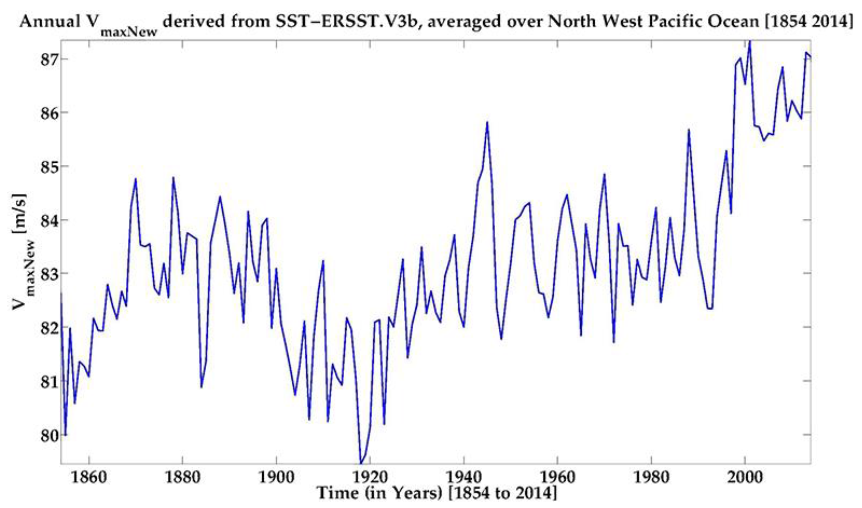
The Northwest Pacific: Graph of V_maxNew in the Northwest Pacific (Figure 11) shows that there has been an interesting long term cycle of rise and fall from 1854 to 1980 after which the TC strengthened sharply. The least active year in terms of TC strength was 1919.

(4)

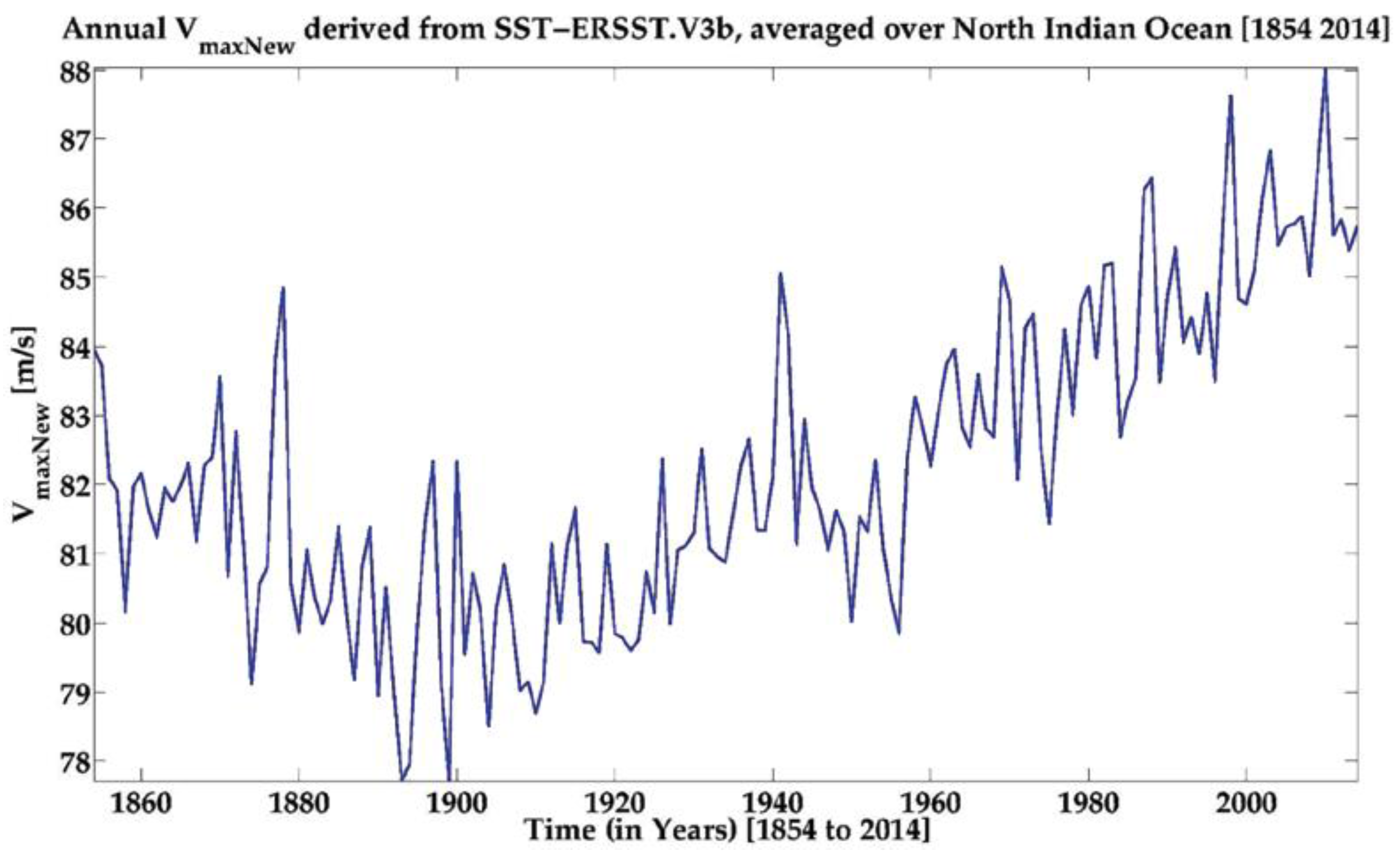
The North Indian Ocean: The North Indian Ocean looks like an active region accommodating various intense tropical storms since early 1990 (Figure 12). Although there was a comparatively dormant period during 1895 to 1990, a dramatic rise is observed thereafter.

(5)

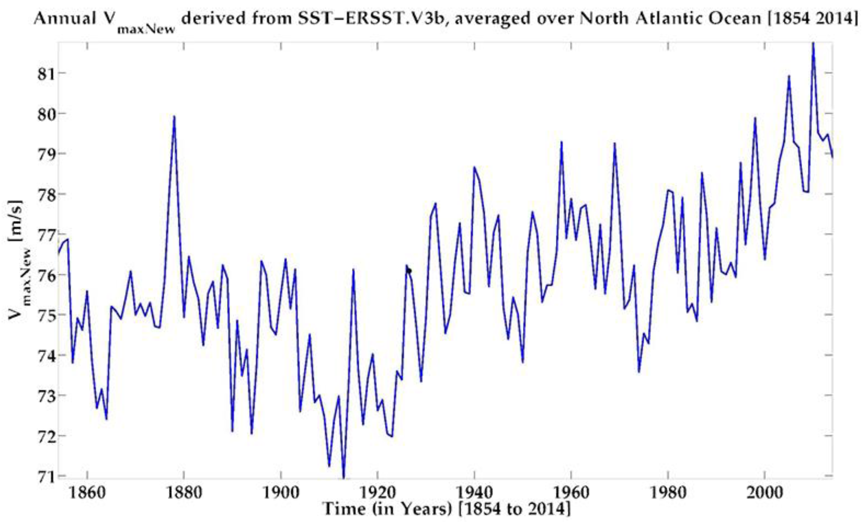
The North Atlantic Ocean: The North Atlantic Ocean seems to drift from moderately active to a dramatically active TC region, in terms of the associated destructive potential (Figure 13). Year 2005 and 2010 marked years of severe tropical storms. The period prior to 1910 was of low cyclone activity.

Of all these discussed ocean basins, the Northwest Pacific and the North Indian Ocean represent the regions of high intensity storms, followed by the North Atlantic. The South Indian Ocean accommodates the least active storms of all the considered oceans. However on an average, the TC intensity in the South Indian Ocean shows gradual growth since 1960. The Southwest Pacific also follows a rising trend in the TC intensity since 1960 onwards.

The Northern Hemispheric oceans can thus be regarded as the more active region for TC intensification, as compared to the Southern Hemisphere.

Decadal Trends: Decadal fluctuations are most prominent in the Southwest Pacific and the North Atlantic. Other oceans show either small cycles or a very long cycle as in the Northwest Pacific. All the TC prone basins however show a dramatic rise since 1970. It is worth mentioning that here we only briefly describe the observed overall tendency. However, trend detection is a separate subject of investigation where it is necessary to isolate the different components from the time series (seasonal, error in data and the trend) and quantify the trend for a chosen time period e.g., decadal or centennial.

To conclude this section, similar to the steep rise predicted using a full calculation model [47,48], statistically simulated wind speeds show a sharp rise post the satellite era, after 1970s.

6. Summary and Future Work

The three considered SST datasets support the notion that in tropical cyclone-prone areas, oceanic-atmospheric temperature contrast and, thus, SST strongly contributes to maximum surface wind speeds of TCs. This high correlation is explained by the enthalpy exchange process between the sea surface and the atmospheric profile above it, considering the TC system as a natural Carnot engine. The higher this contrast is, the greater is the energy transferred upwards during cyclone genesis. According to the simple linear model developed based on significant correlations, it is possible to determine TC intensity primarily using only SST values at the corresponding time scales, with somewhat suboptimal but acceptable performance, when other data (SLP, atmospheric profile) are missing. In this paper, we explored this possibility using a simplistic approach, where the results indicate that they match another evolved models to a first degree of approximation for climatologically averaged datasets. This assumes importance in light of the fact that it is challenging to obtain parameters like mixing ratio and other atmospheric temperature profile variables at remote, less accessible locations or for retrospective studies during the pre-satellite era. In our future work, we will first extend the method to reduce the scatter using other parameters and then test its performance on different categories of tropical cyclones, using available data for known major cyclones.

Tropical cyclone intensities vary in the different ocean basins. Changes in the simulated surface wind speeds under 2× and 1× CO₂ levels show higher values for the Northeast Pacific and the North Atlantic Oceans and comparatively lower values for the North Indian and the Northwest Pacific Oceans (Figure 3). This situation reverses in the Southern Hemisphere with higher wind speeds in the Southwest Pacific and the South Indian Oceans than that in the South Atlantic and the East Pacific. Also, statistically significant differences of the maximum wind speed under a double CO₂ climate appear in the Southeast Pacific. Spatial distribution of simulated wind speeds in the Pacific Ocean shows patterns similar to the El Niño Southern Oscillation (ENSO) warm pool and cold tongue. This pattern is unambiguously visible in reanalysis and model derived wind speeds as well. Variability of these wind speed structures indicates a possible connection of ENSO and maximum sustained winds. This aspect needs more rigorous investigation and is beyond the scope of this work.

Interestingly, correlation between oceanic atmospheric temperature differences and simulated surface wind speeds is stronger for major cyclones (belonging to category 3 or more). That is, stronger storms follow the linear relationship obtained through this model, better than weaker storms. One possible explanation of this could be the role of WISHE (Wind-Induced Surface Heat Exchange) in deciding the weaker or stronger storms (in terms of V_max) and hence their relation with the oceanic atmospheric temperature difference.

Model analysis shows that high surface wind speeds associated with stronger TCs are located in relatively lower, up to approximately 20° latitudes, in both the hemispheres. Also, the Northern Hemisphere warms more and usually experiences higher cyclone winds than the Southern Hemisphere.

The North Atlantic and the East Pacific Ocean basins are the regions more prone to high category storms than the West Pacific and the Indian Ocean. The peculiarity of a vast land region, north of the Indian Ocean, could account for the relatively diminished heat energy available to feed a TC, in comparison to other oceans.

In a futuristic prediction by a climate model, both tropical SST and a storm’s surface wind speeds increase. The computed difference between the two V_max values (with and without when using a doubled CO₂ scenario) in the Indian Ocean, the West Pacific and the North Atlantic Ocean indicate a rise in PDI when doubling CO₂ in our environment. In addition, significant differences of maximum wind speeds under a double CO₂ climate also appear in the Southeast Pacific.

The following is a summary of the key observations: (a) Correlation between the ocean temperature and V_max is stronger for higher values of the latter (figure not shown); (b) Northern Hemisphere shows comparatively stronger storms than the Southern Hemisphere, owing to a higher ocean warming in the Northern Hemisphere; (c) The North Atlantic and the Pacific Oceans are prone to stronger storms; (d) In a futuristic scenario of doubled CO₂, both SST and V_max increases. The oceans more prone to such intensification are the North Indian, the West Pacific and the Southeast Pacific basins; (e) Tropical cyclone intensity is highly dependent on ocean temperature. SST can be considered as one of the main driving forces for tropical cyclone intensification. Hence, in the absence of other parameters, we can use SST to simulate tropical cyclone intensity to a reasonable extent for global tropical oceans as has also been demonstrated by previous case studies (cf., [49]).

The following are the main limitations of this work: (a) This work employed the WISHE model approach which is also debated in some research results [49]. Thus we suggest a further investigation using a model closer to the non-axisymmetric spin-up state of an ideal tropical cyclone; (b) The developed model is based on SST alone which has an advantage while studying tropical cyclone intensity at locations where all the needed atmospheric profiles are missing and SST is available. However, any error in SST will be propagated to the estimated wind speeds as there is no mechanism to prevent error propagation in such an overly simplistic approach; (c) The current validation is performed as follows: Verification using two independent SSTs, other than the one used to derive the equation and comparison against Emanuel’s model output. However, our results are not compared against actual observations, which remain the subject for future studies. Nevertheless, it should be noted that no matter what we validate against (product minus reference), the statistical numbers (e.g., mean, standard deviation) have contributions from both the “target product” and the “reference product” and are therefore subject to some error. To alleviate this issue and characterize true product-specific random errors, a triple-collocation method (cf., [50] employed on near-surface wind fields) needs to be explored in an extension of this work.

References

1. Bister, M.; Emanuel, K.A. Low frequency variability of tropical cyclone potential intensity 1. Interannual to interdecadal variability. J. Geophys. Res. Atmos. 2002, 107. [Google Scholar] [CrossRef]
2. Emanuel, K. Environmental factors affecting tropical cyclone power dissipation. J. Clim. 2007, 20, 5497–5509. [Google Scholar] [CrossRef]
3. Emanuel, K. Increasing destructiveness of tropical cyclones over the past 30 years. Nature 2005, 436, 686–688. [Google Scholar] [CrossRef] [PubMed]
4. Bryan, G.H.; Rotunno, R. The maximum intensity of tropical cyclones in axisymmetric numerical model simulations. Mon. Weather Rev. 2009, 137, 1770–1789. [Google Scholar] [CrossRef]
5. Emanuel, K.A. An air sea interaction theory for tropical cylones. Part I: Steady-state maintenance. J. Atmos. Sci. 1986, 43, 585–604. [Google Scholar] [CrossRef]
6. Emanuel, K.A. The maximum intensity of hurricanes. J. Atmos. Sci. 1988, 45, 1143–1155. [Google Scholar] [CrossRef]
7. Emanuel, K.A. Sensitivity of tropical cyclones to surface exchange coefficients and a revised steady-state model incorporating eye dynamics. J. Atmos. Sci. 1995, 52, 3969–3976. [Google Scholar] [CrossRef]
8. Simpson, J.; Ritchie, E.; Holland, G.J.; Halverson, J.; Stewart, S. Mesoscale interactions in tropical cyclone genesis. Mon. Weather Rev. 1997, 125, 2643–2661. [Google Scholar] [CrossRef]
9. Rotunno, R.; Emanuel, K.A. An air-sea interaction theory for tropical cyclones. Part II: Evolutionary study using a non-hydrostatic axisymmetrical numerical-model. J. Atmos. Sci. 1987, 44, 542–561. [Google Scholar] [CrossRef]
10. Persing, J.; Montgomery, M.T. Is environmental CAPE important in the determination of maximum possible hurricane intensity? J. Atmos. Sci. 2005, 62, 542–550. [Google Scholar] [CrossRef]
11. Demaria, M.; Kaplan, J. Sea-surface temperature and the maximum intensity of Atlantic tropical Cyclones. J. Clim. 1994, 7, 1324–1334. [Google Scholar] [CrossRef]
12. Zeng, Z.; Wang, Y.; Wu, C.-C. Environmental dynamical control of tropical cyclone intensity—An observational study. Mon. Weather Rev. 2007, 135, 38–59. [Google Scholar] [CrossRef]
13. Whitney, L.D.; Hobgood, J.S. The relationship between sea surface temperatures and maximum intensities of tropical cyclones in the eastern North Pacific Ocean. J. Clim. 1997, 10, 2921–2930. [Google Scholar] [CrossRef]
14. Saunders, M.A.; Harris, A.R. Statistical evidence links exceptional 1995 Atlantic hurricane season to record sea warming. Geophys. Res. Lett. 1997, 24, 1255–1258. [Google Scholar] [CrossRef]
15. Bister, M.; Emanuel, K.A. Dissipative heating and hurricane intensity. Meteorol. Atmos. Phys. 1998, 65, 233–240. [Google Scholar] [CrossRef]
16. Emanuel, K.A. The power of a hurricane: An example of reckless driving on the information superhighway. Weather 1999, 54, 107–108. [Google Scholar] [CrossRef]
17. Mallen, K.J.; Montgomery, M.T.; Wang, B. Reexamining the near-core radial structure of the tropical cyclone primary circulation: Implications for vortex resiliency. J. Atmos. Sci. 2005, 62, 408–425. [Google Scholar] [CrossRef]
18. Weatherford, C.L.; Gray, W.M. Typhoon structure as revealed by aircraft reconnaissance. Part I: Data-analysis and climatology. Mon. Weather Rev. 1988, 116, 1032–1043. [Google Scholar] [CrossRef]
19. Powell, M.D.; Vickery, P.J.; Reinhold, T.A. Reduced drag coefficient for high wind speeds in tropical cyclones. Nature 2003, 422, 279–283. [Google Scholar] [CrossRef] [PubMed]
20. Palmen, E. On the formation and structure of tropical hurricanes. Geophysica 1948, 3, 26–38. [Google Scholar]
21. Hebert, C. The hurricane Severity Index—A destructive potential rating system for tropical cyclones. In Proceedings of the 28th Conference on Hurricanes and Tropical Meteorology, Orlando, FL, USA, 27–29 April 2008.
22. Bureau of Meteorology, Australia. What is the Tropical Cyclones Intensity Scale? How is this Different from the USA Intensity Scale? Available online: http://www.bom.gov.au/cyclone/faq/ (accessed on 12 March 2016).
23. Bell, G.D.; Halpert, M.S.; Schnell, R.C.; Higgins, R.W.; Lawrimore, J.; Kousky, V.E.; Tinker, R.; Thiaw, W.; Chelliah, M.; Artusa, A. Climate assessment for 1999. Bull. Am. Meteorol. Soc. 2000, 81, s1–s50. [Google Scholar] [CrossRef]
24. Miller, B.I. On the maximum intensity of hurricanes. J. Meteorol. 1958, 15, 184–195. [Google Scholar] [CrossRef]
25. Shen, W.X.; Tuleya, R.E.; Ginis, I. A sensitivity study of the thermodynamic environment on GFDL model hurricane intensity: Implications for global warming. J. Clim. 2000, 13, 109–121. [Google Scholar] [CrossRef]
26. Holland, G.J. The maximum potential intensity of tropical cyclones. J. Atmos. Sci. 1997, 54, 2519–2541. [Google Scholar] [CrossRef]
27. Sobel, A.H.; Held, I.M.; Bretherton, C.S. The ENSO signal in tropical tropospheric temperature. J. Clim. 2002, 15, 2702–2706. [Google Scholar] [CrossRef]
28. Reynolds, R.W.; Rayner, N.A.; Smith, T.M.; Stokes, D.C.; Wang, W.Q. An improved in situ and satellite SST analysis for climate. J. Clim. 2002, 15, 1609–1625. [Google Scholar] [CrossRef]
29. NOAA Optimum Interpolation (OI) Sea Surface Temperature (SST) V2. Available online: http://www.esrl.noaa.gov/psd/data/gridded/data.noaa.oisst.v2.html (accessed on 2 December 2015).
30. Smith, T.M.; Reynolds, R.W.; Peterson, T.C.; Lawrimore, J. Improvements to NOAA’s historical merged land-ocean surface temperature analysis (1880–2006). J. Clim. 2008, 21, 2283–2296. [Google Scholar] [CrossRef]
31. COBE Sea Surface Temperature Reanalysis. Available online: http://www.esrl.noaa.gov/psd/data/gridded/data.cobe.html (accessed on 3 December 2015).
32. Zhu, T.; Zhang, D.L. The impact of the storm-induced SST cooling on hurricane intensity. Adv. Atmos. Sci. 2006, 23, 14–22. [Google Scholar] [CrossRef]
33. Davis, J.L.; Herring, T.A.; Shapiro, I.I.; Rogers, A.E.E.; Elgered, G. Geodesy by radio interferometry: Effects of atmospheric modeling errors on estimates of baseline length. Radio Sci. 1985, 20, 1593–1607. [Google Scholar] [CrossRef]
34. Bevis, M.; Businger, S.; Herring, T.; Rocken, C.; Anthes, R.; Ware, R. GPS meteorology- Remote sensing of atmospheric water vapor using the Global Positioning System. J. Geophys. Res. 1992, 97, 15787–15801. [Google Scholar] [CrossRef]
35. Collins, M.; Booth, B.B.; Bhaskaran, B.; Harris, G.R.; Murphy, J.M.; Sexton, D.M.; Webb, M.J. Climate model errors, feedbacks and forcings: A comparison of perturbed physics and multi-model ensembles. Clim. Dyn. 2011, 36, 1737–1766. [Google Scholar] [CrossRef]
36. Moore, B.W.; Gates, W.L.; Mata, L.J.; Underdal, R.J.; Stouffer, R.J.; Bolin, B.; Ramirez Rojas, A. Advancing our understanding. In Climate Change 2001: The Scientific Basis, 2nd ed.; Houghton, J.T., Ding, Y., Griggs, D.J., Nouger, M., van der Linden, P.J., Dai, X., Maskell, K., Johnson, C.A., Eds.; Cambridge University Press: Cambridge, UK, 2001; pp. 769–787. [Google Scholar]
37. Kalnay, E.; Kanamitsu, M.; Kistler, R.; Collins, W.; Deaven, D.; Gandin, L.; Iredell, M.; Saha, S.; White, G.; Woollen, J.; et al. The NCEP/NCAR 40-year reanalysis project. Bull. Am. Meteorol. Soc. 1996, 77, 437–471. [Google Scholar] [CrossRef]
38. NCEP/NCAR Reanalysis Monthly Means and Other Derived Variables. Available online: http://www.esrl.noaa.gov/psd/data/gridded/data.ncep.reanalysis.derived.html (accessed on 3 December 2015).
39. Martin, M.; Dash, P.; Ignatov, A.; Banzon, V.; Beggs, H.; Brasnett, B.; Cayula, J.-F.; Cummings, J.; Donlon, C.; Gentemann, C.; et al. Group for High Resolution Sea Surface temperature (GHRSST) analysis fields inter-comparisons. Part 1: A GHRSST multi-product ensemble (GMPE). Deep Sea Res. Part II Top. Stud. Oceanogr. 2012, 77, 21–30. [Google Scholar] [CrossRef]
40. Dash, P.; Ignatov, A.; Martin, M.; Donlon, C.; Brasnett, B.; Reynolds, R.W.; Banzon, V.; Beggs, H.; Cayula, J.-F.; Chao, Y.; et al. Group for High Resolution Sea Surface temperature (GHRSST) analysis fields inter-comparisons. Part 2: Near real time web-based level 4 SST Quality Monitor (L4-SQUAM). Deep Sea Res. Part II Top. Stud. Oceanogr. 2012, 77, 31–43. [Google Scholar] [CrossRef]
41. Met Office Climate Prediction Model: HadCM3. Available online: http://www.metoffice.gov.uk/research/modelling-systems/unified-model/climate-models/hadcm3 (accessed on 3 December 2015).
42. Gordon, C.; Cooper, C.; Senior, C.A.; Banks, H.; Gregory, J.M.; Johns, T.C.; Mitchell, J.F.B.; Wood, R.A. The simulation of SST, sea ice extents and ocean heat transports in a version of the Hadley centre coupled model without flux adjustments. Clim. Dyn. 2001, 16, 147–168. [Google Scholar] [CrossRef]
43. Collins, M.; Tett, S.F.B.; Cooper, C. The internal climate variability of HadCM3, a version of the Hadley centre coupled model without flux adjustments. Clim. Dyn. 2001, 17, 61–81. [Google Scholar] [CrossRef]
44. Efron, B.; Tibshirani, R.J. An Introduction to the Bootstrap; Chapman & Hall: New York, NY, USA, 1993. [Google Scholar]
45. Bell, M.M.; Montgomery, M.T.; Emanuel, K.A. Air-sea enthalpy and momentum exchange at major hurricane wind speeds observed during CBLAST. J. Atmos. Sci. 2012, 69, 3197–3222. [Google Scholar] [CrossRef]
46. Henderson-Sellers, A.; Zhang, H.; Berz, G.; Emanuel, K.; Gray, W.; Landsea, C.; Holland, G.; Lighthill, J.; Shieh, S.L.; Webster, P.; et al. Tropical cyclones and global climate change: A post-IPCC assessment. Bull. Am. Meteorol. Soc. 1998, 79, 19–38. [Google Scholar] [CrossRef]
47. Evans, J.L. Sensitivity of tropical cyclone intensity to sea surface temperature. J. Clim. 1993, 6, 1133–1140. [Google Scholar] [CrossRef]
48. Evans, J.L.; Ryan, B.F.; McGregor, J.L. A numerical exploration of the sensitivity of tropical cyclone rainfall intensity to sea surface temperature. J. Clim. 1994, 7, 616–623. [Google Scholar] [CrossRef]
49. Montgomery, M.T.; Sang, N.V.; Smith, R.K.; Persing, J. Do tropical cyclones intensify by WISHE? Q. J. R. Meteorol. Soc. 2009, 135, 1697–1714. [Google Scholar] [CrossRef] [Green Version]
50. Stoffelen, A. Towards the true near-surface wind speed: Error modeling and calibration using triple collocation. J. Geophys. Res. 1998, 103, 7755–7766. [Google Scholar] [CrossRef]
Figure 1. Comparison of cyclone wind speed Vmax obtained from Emanuel’s model and our simplistic empirical approach with only SST as input. Row-1: Vmax employing Emanuel’s model with reanalysis datasets as inputs: SLP, specific humidity, atmospheric temperature profile and COBE SST; Row-2: VmaxNew employing our approach (Equation 2) with COBE SST; Row-3: Spatial distribution of VmaxNew minus Vmax to visually identify areas of disagreement, considering Vmax as a benchmark (reference); Row-4: Probability density function (PDF) of “∆Vmax = VmaxNewVmax”. Statistical parameters (number of Vmax matches, minimum, maximum, mean, standard deviation, root mean square difference), a Gaussian fit, X~N (mean, Std Dev) and number of grids beyond “Mean ± 4×Std Deviation”, henceforth called ‘extreme grids’ are also annotated on the PDF.
Climate 04 00030 g001
Figure 2. Time-averaged tropical SST from ERSST.V3b dataset.
Climate 04 00030 g002
Figure 3. Change in tropical cyclone wind speeds, VmaxNew, on doubling CO2 scenario.
Climate 04 00030 g003
Figure 4. Wavelet power spectrum of VmaxNew in the North Indian Ocean highlighting temporal patterns of occurrence of maximum wind speeds.
Climate 04 00030 g004
Figure 5. Wavelet power spectrum of VmaxNew in the Southwest Pacific Ocean highlighting temporal patterns of occurrence of maximum wind speeds.
Climate 04 00030 g005
Figure 6. Wavelet power spectrum of VmaxNew in the North Atlantic Ocean.
Climate 04 00030 g006
Figure 7. Wavelet power spectrum of VmaxNew in the Northwest Pacific.
Climate 04 00030 g007
Figure 8. Wavelet power spectrum of VmaxNew in the Southern Indian Ocean.
Climate 04 00030 g008
Figure 9. Time series of Simulated TC wind speed VmaxNew in the Southwest Pacific.
Climate 04 00030 g009
Figure 10. Time series of Simulated TC wind speed VmaxNew in the South Indian Ocean.
Climate 04 00030 g010
Figure 11. Time series of Simulated TC wind speed VmaxNew in the Northwest Pacific.
Climate 04 00030 g011
Figure 12. Time series of Simulated TC wind speed VmaxNew in the North Indian Ocean.
Climate 04 00030 g012
Figure 13. Time series of Simulated TC wind speed VmaxNew in North Atlantic Ocean.
Climate 04 00030 g013