Climate Change Impacts on Streamflow Drought: A Case Study in Tseng-Wen Reservoir Catchment in Southern Taiwan

Abstract

The study aims to assess climate change impacts on streamflow drought in a catchment upstream of Tseng-Wen Reservoir which is the main water supplier in southern Taiwan. A singular-value-decomposition statistical downscaling method and a stochastic weather generator were applied to six different general circulation models for rainfall and temperature downscaling. Two emission climate change scenarios (A1B and B1) were used for rainfall and temperature projections during the two periods, 2010–2045 and 2081–2100. After rainfall and temperature projections, the HBV-based hydrological model was used to simulate future streamflows. By using the threshold level method, the characteristics of streamflow drought during the baseline period (1975–2000) and the future periods were calculated and compared. Important findings include: (1) the start and end times of scenario droughts occur earlier than those of baseline droughts; (2) streamflow under future scenarios during the dry period tends to decrease in January and February, but to increase in March and April; and (3) most of general circulation models’ results support that the drought duration and magnitude tend to decrease for a given return period in the future, and the occurrence probability of severer drought tends to decrease.

1. Introduction

A drought is a prolonged period of water deficit, and typically occurs when an area receives precipitation below usual levels for months. Droughts may develop during or following periods of low accumulated precipitation relative to normal conditions and is exacerbated by high temperatures. As a drought develops, the lack of rainfall leads to persistently dry conditions, low soil moisture, low river flows, reduced storage in reservoirs and less groundwater recharge [1]. Although Taiwan has abundant precipitation (annual average of about 2510 mm), it is a region prone to droughts due to uneven temporal distribution of precipitation and small storage capacity of man-made reservoirs. Yu et al. [2] found that annual rainfall in southern Taiwan has decreased significantly during the past century. Chen et al. [3] investigated historical trends of meteorological drought by using long-term precipitation records and found that the incidence of meteorological drought has increased in southern Taiwan since around 1960 due to the decreasing trend of rainfall. The study aims to investigate streamflow droughts, defined by the threshold level approach [4], in the Tseng-Wen Reservoir catchment in southern Taiwan to understand how the likelihood of droughts will change under climate change scenarios.

General circulation models (GCMs) are used to assess the possible changes of climate in the future by modeling the effect of particular future emission scenarios of greenhouse gases on the climate [5]. Generally, GCMs are of low resolutions. Therefore, GCMs’ outputs need to be combined with a downscaling technique to provide spatially detailed information to resolve regional details. Fowler et al. [6] reviewed the current downscaling literature, examining developments in the downscaling field specifically for hydrological impacts. There are two kinds of downscaling methods, i.e., statistical downscaling and dynamic downscaling. Statistical downscaling methods construct a statistical relationship between large-scale GCM outputs and local weather variables, and dynamic downscaling methods use high-resolution regional climate models with boundary conditions provided by a GCM to obtain local weather variables. Wilby and Wigley [7] made a comparative summary of the relative merits of statistical and dynamical downscaling techniques. Although both statistical and dynamic downscaling methods have their own advantages, statistical downscaling models were more commonly used in hydrological studies due to their less computational demand [8]. In this study, a statistical downscaling approach was applied by using the singular value decomposition scheme [9] to downscale the monthly precipitation from GCMs under climate change scenarios. The downscaling of monthly temperature under different scenarios is retrieved from the Global Change Research Center, National Taiwan University [10]. The projected changes of monthly precipitation and monthly temperature were then used in a weather generator to project the daily precipitation and daily temperature. After generation of daily precipitation and temperature under climate change scenarios, a conceptual hydrological model was used to simulate the streamflow under future scenarios for drought analysis.

In this work, an HBV-based model [11,12] was employed to simulate daily streamflow under future scenarios. The HBV model was designed by the Swedish Meteorological and Hydrological Institute, and has been successfully applied in over 30 countries [13,14,15,16]. This model was originally developed for use in Scandinavian catchments but has also been proven to work well in tropical and subtropical areas. For example, this model performs well in simulating daily discharge in Taiwan [11]. The HBV model has also been successfully employed to investigate the impact of climate change on water resources [12,17,18,19,20].

The rest of this paper is organized as follows. Section 2 introduces the study site and the data that is available for use in this research. Section 3 describes the techniques of spatial and temporal statistical downscaling, the hydrological model (i.e., the HBV-based model), and the threshold level approach for drought event definition. Section 4 represents the results of daily rainfall and temperature downscaling, calibration and verification of the HBV-based model, the changes in drought characteristics, and drought frequency analysis. Conclusions and future work are finally drawn in Section 5.

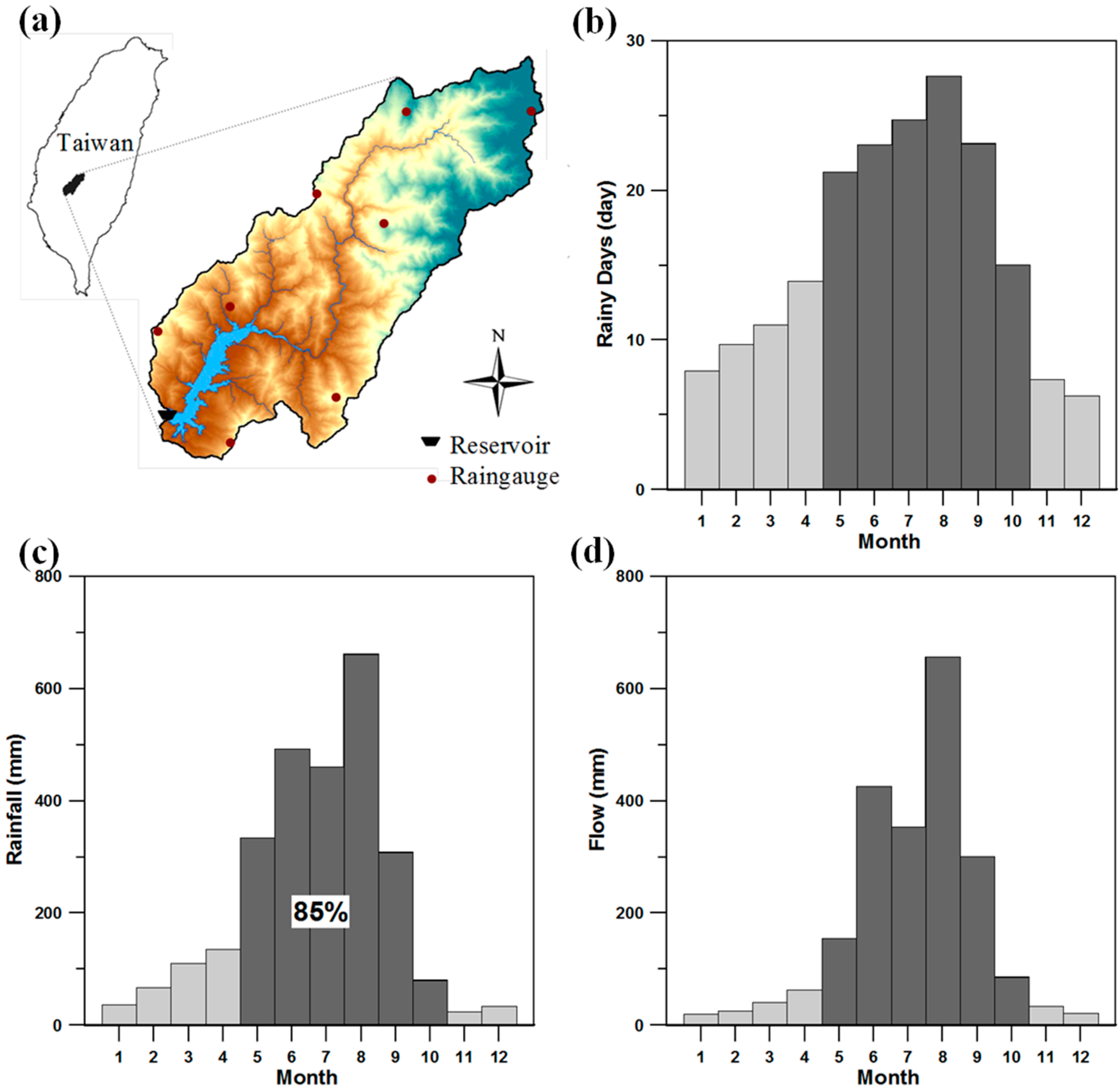
2. Study Area and Data Set

The catchment of Tseng-Wen Reservoir, as shown in Figure 1a, is the study area of this work. With a storage capacity of about 7.8 × 10⁸ m³, Tseng-Wen Reservoir is the largest reservoir in Taiwan and has multiple functions of meeting the water demands for agriculture, domestic use, flood control, and hydropower generation. Tseng-Wen Reservoir catchment encloses an area of 481 km², and has a relief of 157 to 3514 m above the sea level. The mean annual precipitation is about 2744 mm and the mean annual runoff is about 2182 mm during 1975–2000. The study area receives temporally uneven precipitation. Around 85% of annual precipitation occurs during the period from May to October (wet period) but only 15% of annual precipitation occurs from November to April (dry period). The mean monthly rainy days, rainfall, and inflow for each month during 1975–2000 are shown in Figure 1b–d, respectively, which reveal the obvious difference between the wet and dry seasons. Recently, the shortage of water resource during the dry period has often caused the paddy field to lie fallow. Therefore, it is of great concern whether the distribution of water resources during this period is influenced by climate change.

Climate and hydrological data used in this work contain local-scale and large-scale data. Local-scale data on a daily basis, including precipitation, streamflow (i.e., naturalized reservoir inflow) and temperature continuously from 1975 to 2008, are provided by Water Resources Agency in Taiwan. The daily precipitations are available from eight raingauges as shown in Figure 1a, from which areal precipitations on the Tseng-Wen Reservoir catchment were computed using the Thiessen polygon method.

Large-scale data, i.e., GCMs data, were downloaded from the Data Distribution Center of the United Nations Intergovernmental Panel on Climate Change. The climate scenarios describe the emission conditions of greenhouse gases and more details are given in the report of IPCC [21]. Different scenarios used were 20C3M for historical climate, and A1B and B1 for future climate. Generally speaking, 20C3M is the scenario to represent past climate, A1B is currently regarded as the most likely climate scenario in the future and B1 describes a convergent world in which the impact on climate change is less significant than A1B.

Rainfall during typhoon and Meiyu seasons is the major source for seasonal precipitation in Taiwan. A coupled GCM (CGCM) that can simulate tropical cyclone index or large-scale circulation reasonably would be the candidate for downscaling study over Taiwan. Tropical cyclone (TC) activity in nine CGCMs submitted to IPCC AR4 is evaluated by means of yearly genesis parameter (YGP) and convective-YGP index [22]. On the other hand, the ability of CGCMs in simulating large-scale circulation pattern in East Asia is given by Min et al. [23] and Kitoh and Uchiyama [24]. As a result, six models mentioned in these literatures with reasonable performance are taken into account in the present study. Table 1 lists the summary of six used GCMs.

Figure 1. The basic information of the study area: (a) Tseng-Wen Reservoir catchment; (b) rainy days; (c) mean monthly rainfall; and (d) mean monthly flow.

Figure 1. The basic information of the study area: (a) Tseng-Wen Reservoir catchment; (b) rainy days; (c) mean monthly rainfall; and (d) mean monthly flow.

Table 1. Summary of the GCMs used in the study.

Model Code	Model Name	Country	Resolution
GCM-1	CGCM3.1(T63)	Canada	T63, L31
GCM-2	CSIRO-Mk3.0	Australia	T63, L18
GCM-3	ECHAM5/MPI-OM	Germany	T63, L31
GCM-4	GFDL-CM2.0	USA	2° × 2.5°, L24
GCM-5	GFDL-CM2.1	USA	2° × 2.5°, L24
GCM-6	MIROC3.2(hires)	Japan	T106, L56

Table 1. Summary of the GCMs used in the study.

Model Code	Model Name	Country	Resolution
GCM-1	CGCM3.1(T63)	Canada	T63, L31
GCM-2	CSIRO-Mk3.0	Australia	T63, L18
GCM-3	ECHAM5/MPI-OM	Germany	T63, L31
GCM-4	GFDL-CM2.0	USA	2° × 2.5°, L24
GCM-5	GFDL-CM2.1	USA	2° × 2.5°, L24
GCM-6	MIROC3.2(hires)	Japan	T106, L56

A time period with a length of 20–30 years is usually used for presenting the average climate condition during the period. Based on the common decision of the project teams in Taiwan who executed the studies on assessing the potential impacts of climate change on hydrology, three periods of 1975–2000, 2010–2045 and 2081–2100 were defined as the baseline, near-term and long-term periods, respectively.

3. Methodology

3.1. Spatial and Temporal Statistical Downscaling

GCMs are the main tool to project climate changes through the prescribed emission scenarios. However, due to the coarse resolution, GCMs are not able to represent regional topography and land-sea contrast properly, making local climate projection a big challenge. Thus, a two-stage statistical downscaling method was applied to generate future daily precipitation data from climate outputs run by six GCMs. In the first stage, spatial statistical downscaling was applied by using the singular value decomposition (SVD) scheme [9] to downscale the monthly precipitation form GCM to catchment scale. Monthly temperature downscaling results were obtained from Global Change Research Center, National Taiwan University [10]. In the second stage, temporal statistical downscaling was applied. In the temporal statistical downscaling, the projected changes of monthly precipitation and monthly temperature were further used in a weather generator to produce the daily precipitation and daily temperature. Daily data are more practical for hydrological purpose. After the daily precipitation and daily temperature are generated, the hydrological model uses them as inputs to simulate daily streamflows.

Spatial statistical downscaling provides relationships between local and large-scale variables to overcome the drawback of GCMs’ coarse resolution. The first step of spatial statistical downscaling is data reconstruction by the empirical orthogonal functions to filter off noises. This method is the same as applying principal components analysis. Then the SVD is applied to extract coupled patterns between local precipitation and large-scale variables, which can be expressed in the following equations.

$$Z_{predictor}(t,x)={\displaystyle \sum _{i=1}^m{U}_i(x)\cdot S_i(t)}$$

(1)

$$Z_{predic\tan d}(t,x)={\displaystyle \sum _{i=1}^m{R}_i(x)\cdot K_i(t)}$$

(2)

where $Z_{predictor}(t, x)$ and $Z_{predictand}(t, x)$ are normalized anomaly field pertaining to the large-scale circulation and the observed station rainfall, respectively; m is the total number of SVD modes; $U_i(x)$ and $R_i(x)$ denote respectively the singular vector of the predictor and the singular vector of the predictand in the i-th mode; and $S_i(t)$ and $K_i(t)$ indicate the time series of expansion coefficient of the i-th SVD mode regarding the predictor and the predictand.

The downscaling results can then be obtained by applying GCMs projection data to the following transfer functions.

$$S_i(t_p)={\displaystyle \sum _{j=1}^x{Z}_{predictor}(t_p,j)\cdot U_i(j)}$$

(3)

$$PRJ(t_p,x)={\displaystyle \sum _{i=1}^n{S}_i(t_p)\cdot R_i(x)}$$

(4)

where $PRJ(t_p, x)$ represents the projected predictand; $t_p$ stands for the projection time horizon; and n denotes the total number of the SVD modes retained. In this study, the leading ten modes are retained. The details of the method of downscaling can be found in Kim et al. [25] and Feddersen and Andersen [26].

In the second stage of temporal statistical downscaling, a stochastic weather generator was applied to downscale the monthly precipitation, derived in the first stage, to the daily precipitation. The daily precipitation generation is based on procedures proposed by Richardson [27]. The generator uses a Markov chain to model the occurrence of wet or dry days, and then uses a probability distribution to generate the precipitation amount conditional on a wet day modeled by the Markov chain. A first-order two-state Markov chain was used in this work. The occurrence of a dry or wet day is modeled by a transition probability matrix consisting of conditional probabilities, given a previous dry or wet day.

Many probability distributions were applied to generate daily precipitation amount, such as the exponential distribution [28,29], Weibull distribution [12], two-parameter gamma distribution [27,30,31,32,33], and mixed exponential distribution [31,34,35]. Among the probability distributions, the Weibull distribution most appropriately approximates daily rainfall in Taiwan [12]; consequently, this work used the Weibull distribution to generate daily rainfall.

Regarding the daily temperature generation, a first-order autoregressive model was utilized to generate the daily temperature sequences in each month. This daily temperature generation model is expressed as follows:

$$T_k={\mathrm{\mu }}_T+{\mathrm{\rho }}_{1T}\left(T_{k-1}-{\mathrm{\mu }}_T\right)+\sqrt{1-{\mathrm{\rho }}_{1T}^2}{\mathrm{\sigma }}_T{\mathrm{\nu }}_k+\Delta \mathrm{\mu }$$

(5)

where T_k is the temperature on day k; μ_T is the mean temperature in a certain month; σ_T is the standard deviation of daily temperature in the month; ρ_1T is the lag-one autocorrelation coefficient of daily temperature in the month; ν_k is the random standard normal variate, and Δμ is the mean temperature change in the month under a future scenario. Given the parameters, μ_T, σ_T, σ_1T, and Δμ, a daily temperature sequence in a month can be generated by this model.

3.2. Hydrological Model

A continuous hydrologic model was used to simulate future projected streamflow, after the daily precipitation and temperature were obtained in the previous section by the downscaling method. This work used a continuous hydrologic model based on the structure of Hydrologiska Byrans Vattenbalansavdelning (HBV) model [13,14], which was initially designed for use in Scandinavian catchments by the Swedish meteorological and hydrological institute. Yu and Yang [11] adapted the HBV model structure to suit catchments in Taiwan. The HBV-based model uses both an upper and lower tank to model the rainfall-runoff behavior. Model structure mainly consists of three parts: (1) soil moisture module; (2) runoff response mechanism; and (3) water balance functions. Detail description of the HBV-based model, as well as its procedures for calibration and validation in this work, can be found in Yu and Yang [11] and Yu et al. [12].

In the HBV-based model, Hamon’s temperature-dependent equation [36] was used to transform the daily temperature series into the daily potential evapotranspirartion series. The Hamon’s temperature-dependent equation is as:

$$Ep(t)=0.21H{(t)}^2{e}_o(t)/[T(t)+273]$$

(6)

where E_p(t) is the potential evapotranspiration (mm/day) on day t; H(t) is the sunshine duration (hour) on day t; e_o(t) is the saturated vapor pressure (milibar) on day t; T(t) is the mean temperature (°C) on day t. Data of H(t) are available at the Ali-Shan meteorological station near the study area, and e_o(t) can be estimated by the following empirical equation.

$$e_o(t)=33.8639\times ({(0.00738\times T(t)+0.8072)}^8-0.000019\times \left| 1.8\cdot T(t)+48 \right|+0.001316)$$

(7)

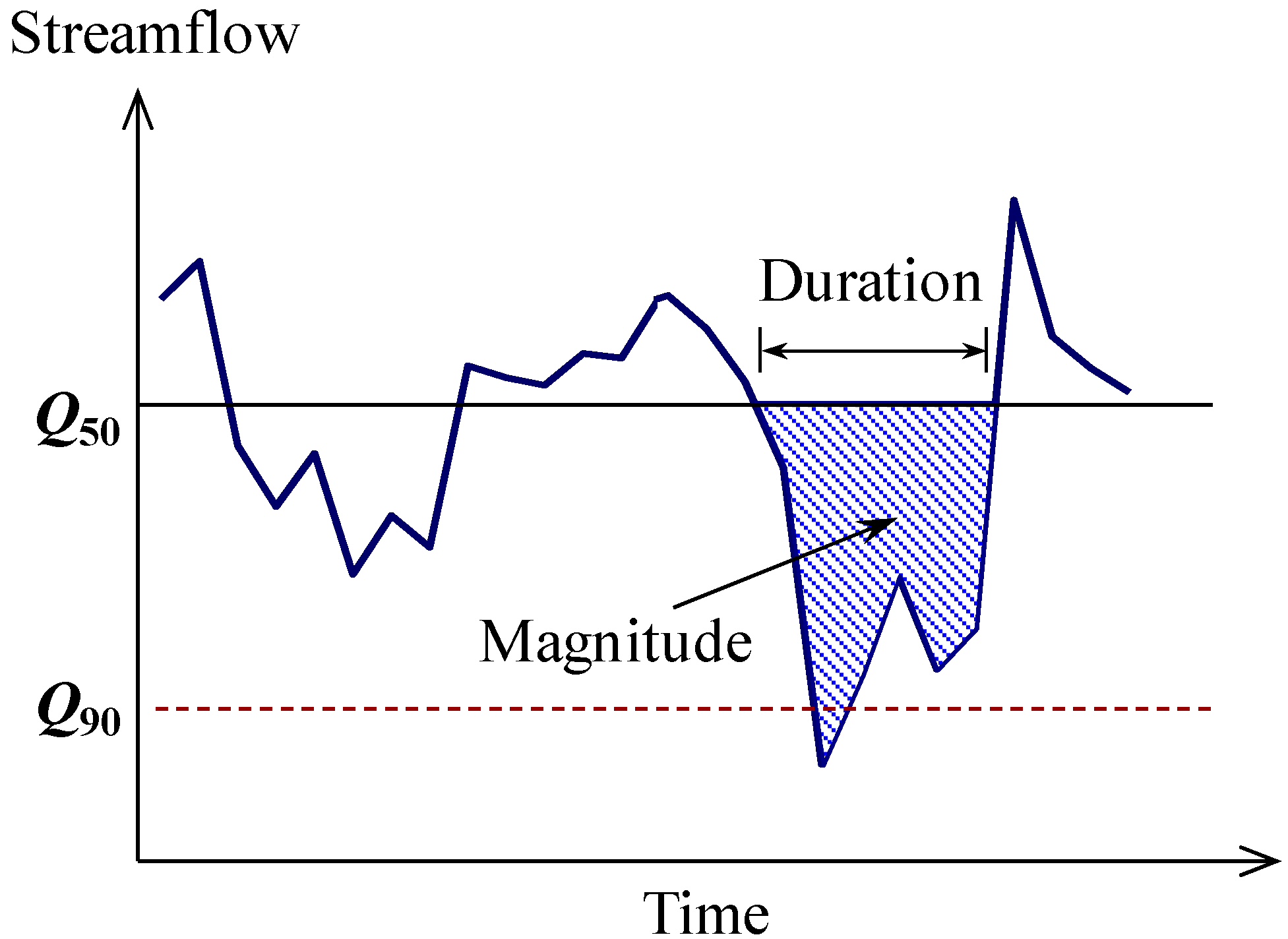
3.3. Threshold Level Method for Drought Event Definition

The categories of droughts are frequently used as follows [37]: climatological drought (deficit in precipitation), agro-meteorological drought (deficit in soil water), river flow drought (deficit in river discharge), groundwater drought (deficit in groundwater storage), and operational drought (conflict of water shortage and water management demands). Within the present study the concept of river flow (or say streamflow) drought is adopted.

The threshold level method proposed by Yevjevich [4] is the most commonly applied approach to drought studies, such as [38,39,40,41,42,43]. The choice of the threshold level is important for the results of a drought study. Besides the option for a constant threshold value for all data over time or for a variable threshold (e.g., fluctuating on a monthly or seasonal basis), the value of the threshold level is highly significant. A threshold level which is too low might lead to a high number of no-drought years making the few identified drought events statistically uncertain to evaluate. On the other hand, with a high threshold level the likelihood for a series of small single drought events being combined into one severe multi-year drought (drought lasting longer than a year) increases [44]. To prevent the aforementioned conditions from occurring, a proper choice of threshold level should be made.

Figure 2. Definition of streamflow drought.

Figure 2. Definition of streamflow drought.

In order to study the features of major streamflow drought, this work defines a streamflow drought based on the annual flow duration curve from which the 50-percentile flow (Q₅₀) and 90-percentile flow (Q₉₀) are selected. A streamflow drought is a low flow event when streamflow series is continuously below the 50-percentile flow (Q₅₀) and the minimum flow during the period is less than the 90-percentile flow (Q₉₀) (Figure 2). The Q₉₀ is required here to avoid minor drought events. Once a drought event is specified, drought characteristic can be quantified. Drought frequency (time/year) is the times of drought occurrence per year. Drought duration (day) is the time period between the start and the end of a drought. Drought magnitude (mm) is the total amount of streamflow deficit, expressed in depth. During a streamflow drought, the daily streamflow deficit is calculated by Q₅₀ minus the daily flow for each day. Then, the drought magnitude can be obtained by summing up the entire daily streamflow deficits during a drought.

4. Results

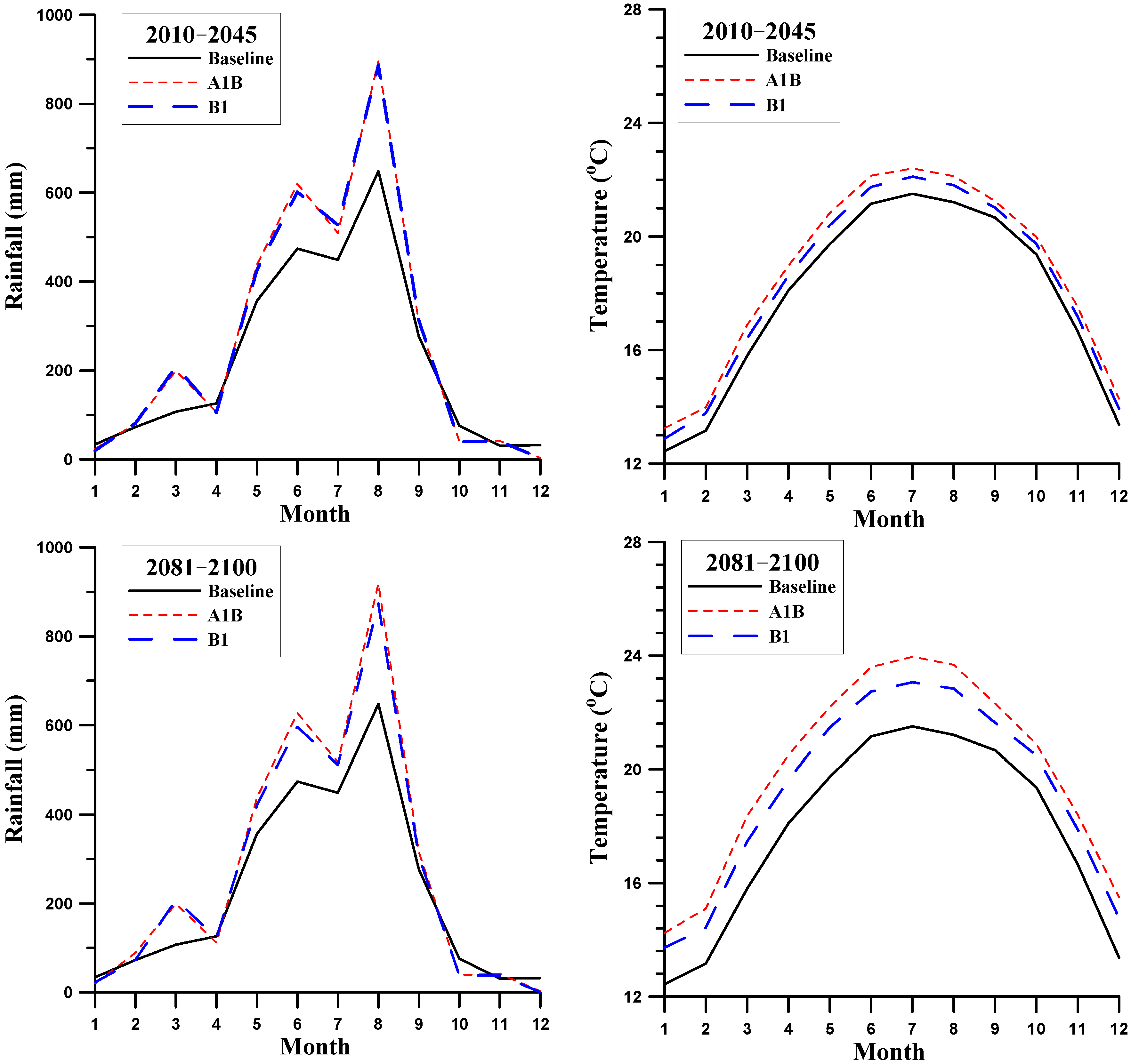
4.1. Precipitation and Temperature Downscaling

The analysis from Chu and Yu [45] demonstrated that the sea level pressure (SLP) and the meridional wind field at 850 hPa (V850) are appropriate predictors for downscaling precipitation over Taiwan. Thus, the two large-scale variables, SLP and V850, both of which are taken from six GCMs involving 20C3M, A1B, and B1 scenarios, are used as predictors for downscaling in this work. The 20C3M scenario is used to reproduce historical climate condition. GCMs’ performance can be evaluated by comparing downscaling results and observation data during 1975–2000. In Figure 3, the left panel presents observation data and downscaling results (under 20C3M scenario) during the period of 1975–2000, indicating that the downscaling results can capture the rainfall pattern of observation data. The Gerrity skill score (GSS), proposed by Gerrity [46], is applied to evaluate the performance of GCM. GSS is easy to construct and, what is noteworthy, equitable, giving rewards and penalties reasonably to the forecast skill. The above mentioned points make GSS a skill score for categorical deterministic forecast recommended by the World Meteorological Organization (WMO) in the standardized verification system for long-range forecasts [47] (WMO 2002). The GSS used herein is only for inspecting monthly-rainfall downscaling performance of the selected GCMs during the baseline period under 20C3M scenario. The GSS value above zero stands for skillful downscaling performance. In Figure 3, the right panel shows that almost all GCMs have a reasonable simulation.

After spatial downscaling process, change rates of monthly precipitation from 20C3M to A1B and B1 scenarios can be obtained. Future projections of monthly precipitation under A1B and B1 scenarios can be derived by multiplying these projected change rates and historical monthly rainfall data together. The changes of monthly temperature from 20C3M to A1B and B1 scenarios during the periods of 2010–2045 and 2081–2100, respectively, were derived by the Global Change Research Center at National Taiwan University [10]. Then, future monthly temperatures can be derived by adding the projected changes to the historical monthly temperature. Figure 4 displays the projected monthly rainfall and mean temperature in each month under A1B and B1 scenarios during the periods of 2010–2045 and 2081–2100, respectively. In the figure, the ensemble results (i.e., the mean results) of the six GCMs under A1B and B1 scenarios are presented, and the baseline indicates the projected values during 1975–2000 under 20C3M. The results reveal that the rainfalls during the wet season (May to September) tend to obviously increase. During the dry season (October to April), the rainfalls has no obvious change, except for March in which there exists an increase. The projected mean monthly temperature tends to increase and the increased change in summer is larger than that in winter. Moreover, the increased change under A1B scenario is larger than that under B1 scenario.

Figure 3. (a) Observation and scenario data during the period between 1975 and 2000 and (b) the Gerrity skill scores of each GCM.

Figure 3. (a) Observation and scenario data during the period between 1975 and 2000 and (b) the Gerrity skill scores of each GCM.

Figure 4. Projected monthly rainfall and mean temperature under A1B and B1 scenarios during the periods of 2010–2045 and 2081–2100, respectively.

Figure 4. Projected monthly rainfall and mean temperature under A1B and B1 scenarios during the periods of 2010–2045 and 2081–2100, respectively.

Then, the projected changes of monthly precipitation and temperature were used in the weather generator to produce daily precipitation and temperature under climate change scenarios. Daily precipitation and temperature of a 200-year length were generated by the temporal statistical downscaling methods for baseline and future climate scenarios, respectively.

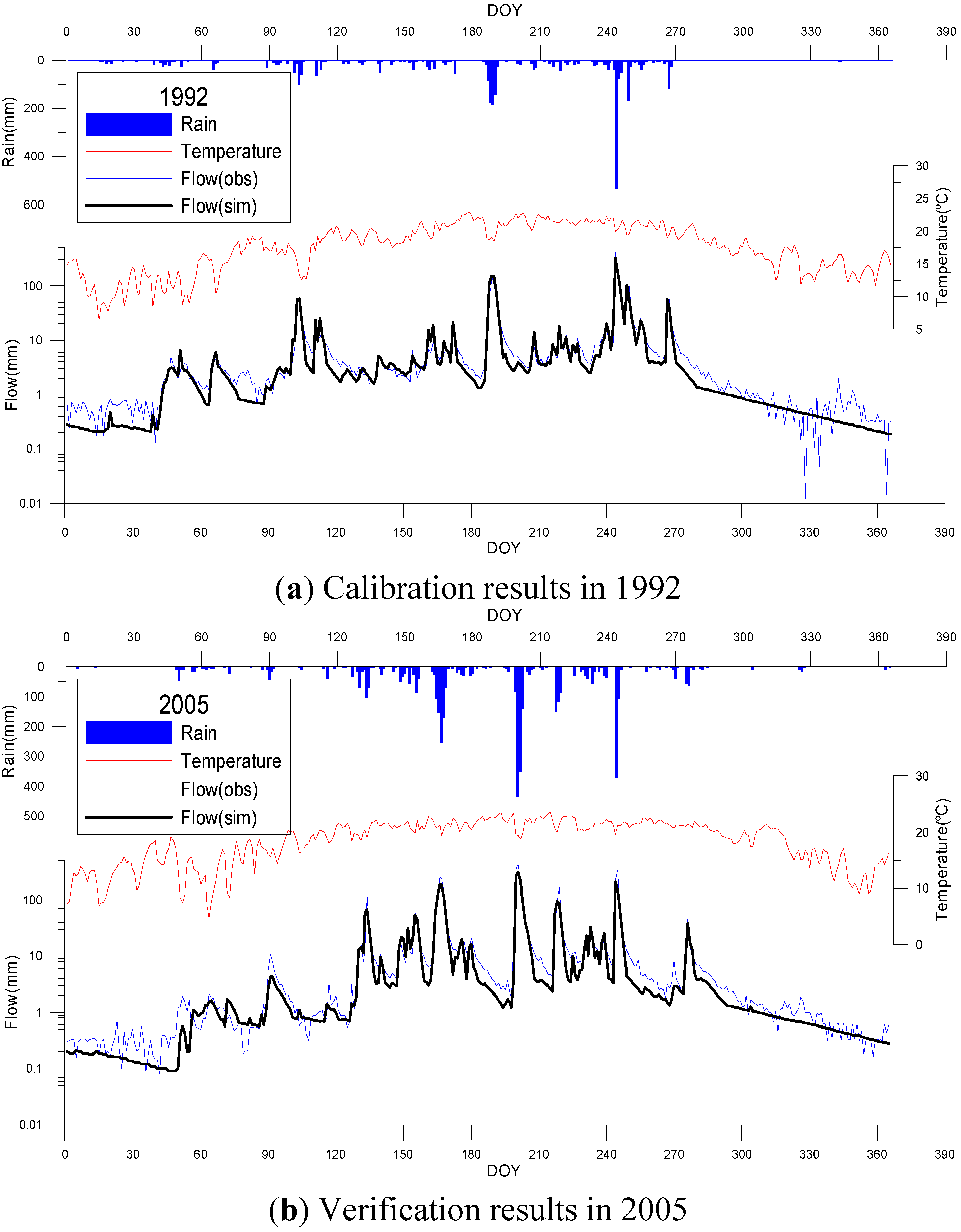
4.2. Calibration and Verification of the HBV-Based Model

During model calibration, the HBV-based model was applied on the Tseng-Wen Reservoir catchment to explore its ability of streamflow simulation. The fuzzy multiple objective functions, proposed by Yu and Yang [11], and the shuffled complex evolution optimization method [48] were used in the study. Historical daily rainfall and flow data from 1975 to 1998 were used for the HBV-based model calibration. The calibrated HBV-based model was further verified by historical daily data from 1999 to 2008. To assess the model performance, three criteria, including the ratio of simulated to observed runoff volumes (Vs/Vo), the root mean squared error (RMSE), and the coefficient of correlation (CC), were calculated pertaining to the calibration and verification periods, respectively. During the calibration period, the values of Vs/Vo, RMSE and CC are 0.86, 9.98 (mm) and 0.86, respectively. During the validation period, the values of Vs/Vo, RMSE and CC are 0.88, 9.90 (mm) and 0.96, respectively. Table 2 lists the values of Vs/Vo, RMSE, and CC for each calibration and validation year. From this table, most of years have good simulation performances. Figure 5 shows the calibration and verification results in 1992 and 2005, respectively. These results reveal the HBV-based model is able to simulate the rainfall-runoff behavior over the study area.

The HBV-based model was then used to simulate future projected streamflow, after the daily precipitation and temperature under the A1B and B1 scenarios were obtained in the previous section by the temporal downscaling. The flow duration curves of the dry season and the wet season, respectively, during the baseline period (1975–2000) and the future period (2010–2045) were shown in Figure 6 to display the influence of projected changes in climate on the hydrological regime. In the figure, the flow duration curve during the future period for each season is the ensemble result of the six GCMs. The future period (2081–2100) has the similar influence with the period (2010–2045) and its figure was not included here. From the average viewpoint, the flows during the wet season increase in future due to the increasing precipitation during the wet season (found in Section 4.1) and the flows during the dry season increase due to the increasing lower tank storage in the HBV-based model during the wet season. These figures implicate the magnitude and duration of the defined drought “may” reduce in future.

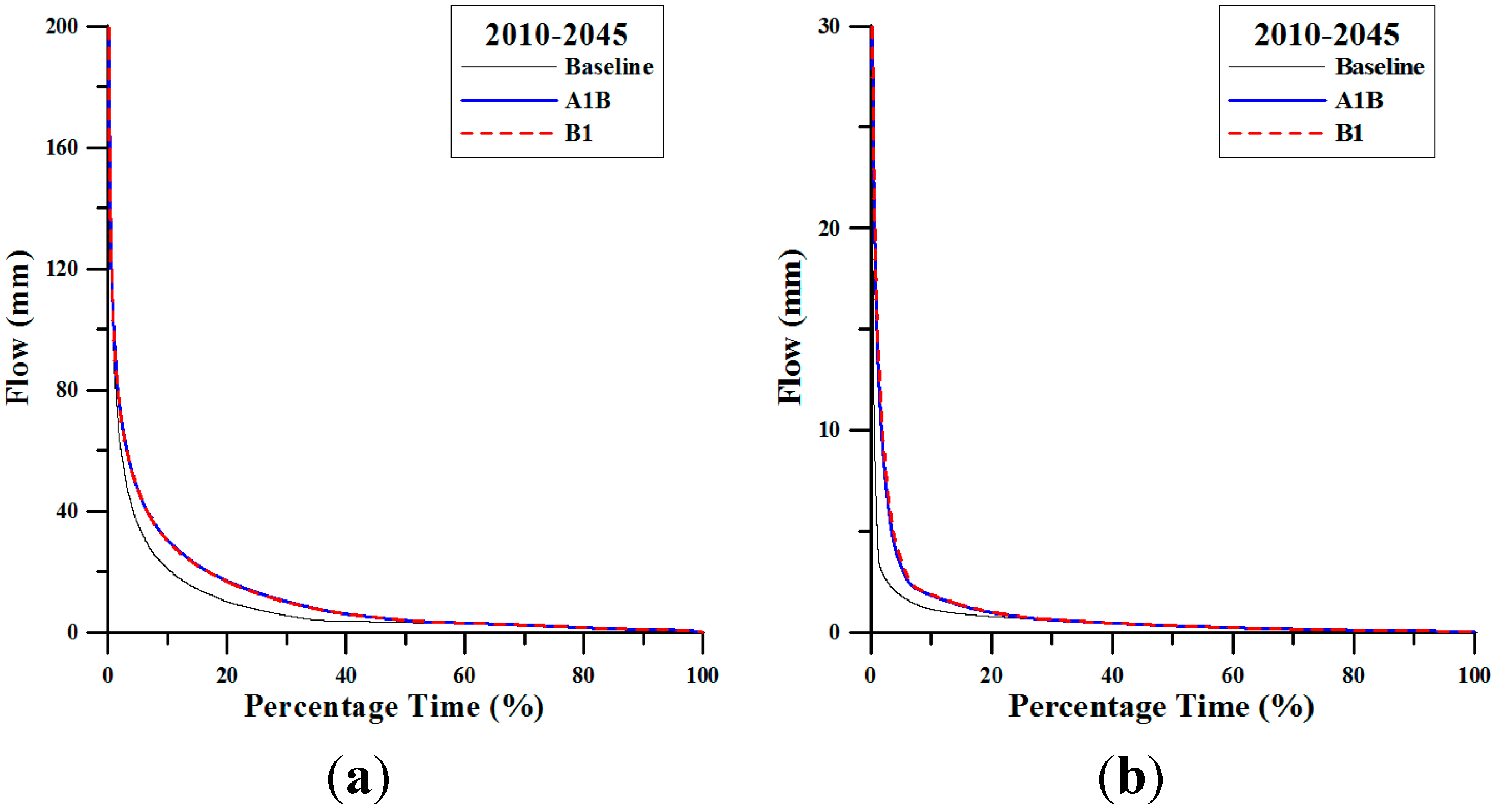
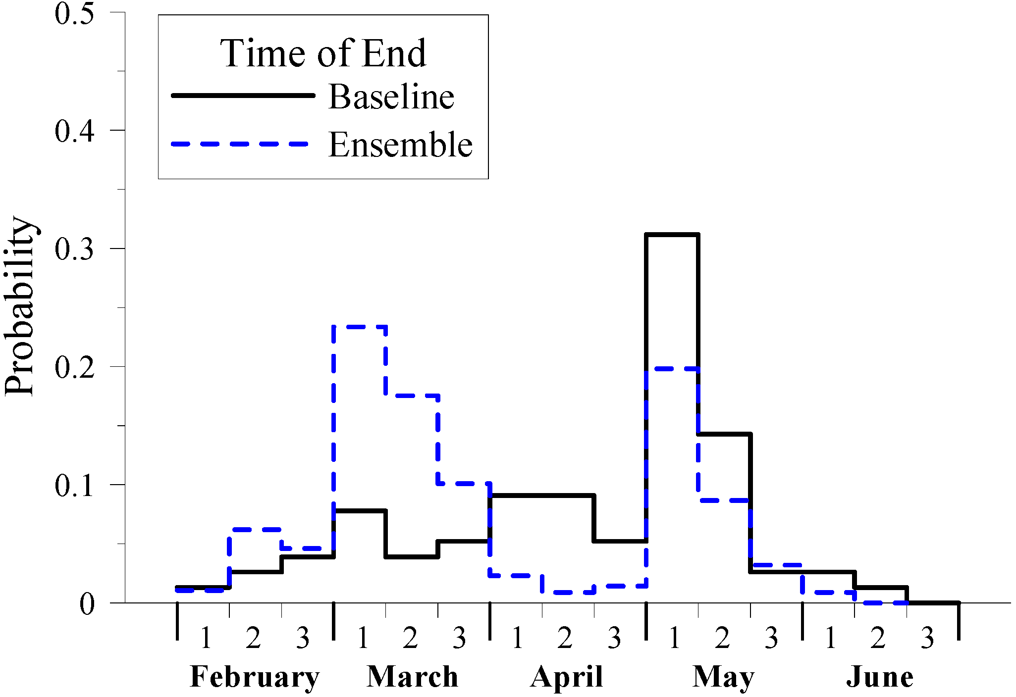
4.3 Changes in Drought Characteristics

The historical streamflow data during the baseline period of 1975–2000 were used to derive the annual flow duration curve from which the Q₅₀ and Q₉₀ were calculated (i.e., 1.24 and 0.16 mm, respectively). Since Q₅₀ and Q₉₀ were used to define a streamflow drought in the present study, the two values for the future scenarios are the same as those for the baseline period. Based on the threshold level method described in the Section 3.3, the drought frequency (0.77 times per year), the mean drought duration (174 days), and the mean drought magnitude (148 mm) can be calculated. These three drought characteristics during the period of 1975–2000 are used as the baseline against which change is compared.

Table 2. Values of three criteria for each year during calibration and validation periods.

Calibration Period				Validation Period
Year	Vs/Vo	RMSE (mm)	CC	Year	Vs/Vo	RMSE (mm)	CC
1975	0.93	23.89	0.46	1999	0.97	5.37	0.91
1976	0.97	20.43	0.74	2000	0.95	3.36	0.94
1977	1.00	25.55	0.60	2001	0.91	10.61	0.93
1978	0.86	15.87	0.70	2002	0.98	2.86	0.94
1979	0.95	8.36	0.90	2003	1.08	3.29	0.94
1980	0.65	6.91	0.84	2004	0.92	6.41	0.99
1981	0.92	9.11	0.97	2005	0.80	15.50	0.96
1982	0.88	4.61	0.97	2006	0.89	11.88	0.96
1983	0.99	5.20	0.94	2007	0.86	11.92	0.97
1984	0.58	5.98	0.96	2008	0.84	13.22	0.97
1985	0.54	10.63	0.92	Total Period	0.88	9.90	0.96
1986	0.59	9.06	0.64
1987	0.93	14.92	0.72
1988	0.60	7.30	0.98
1989	0.77	15.18	0.92
1990	0.72	7.97	0.98
1991	0.87	3.71	0.96
1992	0.96	6.92	0.97
1993	0.98	2.87	0.96
1994	0.94	5.73	0.94
1995	0.96	2.48	0.97
1996	0.82	15.09	0.98
1997	0.97	4.06	0.95
1998	1.01	5.96	0.92
Total Period	0.86	9.98	0.86

Table 2. Values of three criteria for each year during calibration and validation periods.

Calibration Period				Validation Period
Year	Vs/Vo	RMSE (mm)	CC	Year	Vs/Vo	RMSE (mm)	CC
1975	0.93	23.89	0.46	1999	0.97	5.37	0.91
1976	0.97	20.43	0.74	2000	0.95	3.36	0.94
1977	1.00	25.55	0.60	2001	0.91	10.61	0.93
1978	0.86	15.87	0.70	2002	0.98	2.86	0.94
1979	0.95	8.36	0.90	2003	1.08	3.29	0.94
1980	0.65	6.91	0.84	2004	0.92	6.41	0.99
1981	0.92	9.11	0.97	2005	0.80	15.50	0.96
1982	0.88	4.61	0.97	2006	0.89	11.88	0.96
1983	0.99	5.20	0.94	2007	0.86	11.92	0.97
1984	0.58	5.98	0.96	2008	0.84	13.22	0.97
1985	0.54	10.63	0.92	Total Period	0.88	9.90	0.96
1986	0.59	9.06	0.64
1987	0.93	14.92	0.72
1988	0.60	7.30	0.98
1989	0.77	15.18	0.92
1990	0.72	7.97	0.98
1991	0.87	3.71	0.96
1992	0.96	6.92	0.97
1993	0.98	2.87	0.96
1994	0.94	5.73	0.94
1995	0.96	2.48	0.97
1996	0.82	15.09	0.98
1997	0.97	4.06	0.95
1998	1.01	5.96	0.92
Total Period	0.86	9.98	0.86

The change of streamflow drought can be assessed by calculating the differences between historical data (baseline) and projected data under different scenarios (A1B and B1) and during different future periods (2010–2045 and 2081–2100). Table 3 shows drought characteristics, including drought frequency, duration, and magnitude, based on historical data and projected data (results from six GCMs under A1B and B1 scenarios). The scenario droughts become more frequent (0.87 to 1.04 times per year), compared to the frequency of baseline droughts (0.77 times per year). From the ensemble average, the drought frequencies range from 0.94 to 0.97 times per year for different scenarios and different periods, revealing that the future drought frequency tends to increase.

The durations of projected droughts for different GCMs and different future periods are between 128.7 days and 205.9 days. The ensemble averages of projected drought durations are about 160 days for different scenarios and different future periods. As compared to the duration of baseline drought (174 days), the future drought duration decrease about a half month.

Figure 5. Calibration and verification results for the HBV-based model in (a) 1992 and (b) 2005, respectively (DOY: Day of Year).

Figure 5. Calibration and verification results for the HBV-based model in (a) 1992 and (b) 2005, respectively (DOY: Day of Year).

Figure 6. Flow duration curves of the (a) wet season and (b) the dry season during the baseline period and the future period (2010–2045).

Figure 6. Flow duration curves of the (a) wet season and (b) the dry season during the baseline period and the future period (2010–2045).

The tendency of drought magnitude is similar to that of drought duration. The magnitudes of projected droughts are between 102 mm and 196 mm for different GCMs and different future periods. The ensemble averages of projected drought magnitudes are about 140 mm for different scenarios and periods. The future drought magnitude decrease slightly, as compared to the magnitude of baseline drought (148 mm).

To sum up the above analysis, the duration and magnitude of scenario droughts may increase or decrease, as they depend on different GCMs. However, from the ensemble average of GCMs, the results reveal that the duration and magnitude of scenario droughts tend to decrease. Overall, streamflow droughts under future scenarios become more frequent, but their duration and magnitude become more diverse than the baseline droughts.

Figure 7 and Figure 8, respectively, are the time distributions of the start and the end of streamflow droughts, under the A1B scenario for the period of 2010–2045. In the figures, the solid line indicates the baseline drought, and the dash line stands for the ensemble mean of scenario droughts. Figure 7 indicates that baseline droughts more often start during the period from the middle of October (the 2nd 10-day period in October) to early November (the 1st 10day period in November). However, scenario droughts are projected to come earlier and have a high likelihood to start in the middle of October (the 2nd 10-day period in October). Figure 8 reveals that scenario droughts are more likely to end during March that is earlier than the end of baseline droughts more likely in the early May. The time distributions of the start and the end of streamflow droughts pertaining to the B1 scenario and to the period of 2081–2100 are similar. Totally speaking, droughts may start and end earlier in the future.

Table 3. Impact of climate change on streamflow drought characteristics.

Drought Characteristics	Baseline	Future Period	Scenario	Ensemble of GCMs	GCM-1	GCM-2	GCM-3	GCM-4	GCM-5	GCM-6
Frequency (time/year)	0.77	2010–2045	A1B	0.94	0.87	1.02	0.99	0.98	0.89	0.90
			B1	0.96	0.89	0.99	0.95	0.99	0.96	0.95
		2081–2100	A1B	0.97	0.88	1.04	0.99	0.98	0.93	1.00
			B1	0.97	0.91	1.00	0.97	1.00	0.97	0.96
Duration (day)	173.65	2010–2045	A1B	161.2	131.8	193.3	158.8	181.9	149.7	151.6
			B1	161.6	132.9	197.2	160.7	181.3	147.3	150.4
		2081–2100	A1B	160.4	128.7	193.4	151.9	180.0	145.2	163.0
			B1	163.3	132.4	205.9	158.6	184.1	147.4	151.6
Magnitude (mm)	148.44	2010–2045	A1B	139.7	105.3	178.5	137.2	164.6	125.7	126.7
			B1	139.9	105.7	183.0	138.7	162.8	122.3	126.8
		2081–2100	A1B	139.3	102.1	181.6	130.3	161.9	121.1	138.5
			B1	142.9	105.5	195.5	137.7	166.0	125.0	127.9

Table 3. Impact of climate change on streamflow drought characteristics.

Drought Characteristics	Baseline	Future Period	Scenario	Ensemble of GCMs	GCM-1	GCM-2	GCM-3	GCM-4	GCM-5	GCM-6
Frequency (time/year)	0.77	2010–2045	A1B	0.94	0.87	1.02	0.99	0.98	0.89	0.90
			B1	0.96	0.89	0.99	0.95	0.99	0.96	0.95
		2081–2100	A1B	0.97	0.88	1.04	0.99	0.98	0.93	1.00
			B1	0.97	0.91	1.00	0.97	1.00	0.97	0.96
Duration (day)	173.65	2010–2045	A1B	161.2	131.8	193.3	158.8	181.9	149.7	151.6
			B1	161.6	132.9	197.2	160.7	181.3	147.3	150.4
		2081–2100	A1B	160.4	128.7	193.4	151.9	180.0	145.2	163.0
			B1	163.3	132.4	205.9	158.6	184.1	147.4	151.6
Magnitude (mm)	148.44	2010–2045	A1B	139.7	105.3	178.5	137.2	164.6	125.7	126.7
			B1	139.9	105.7	183.0	138.7	162.8	122.3	126.8
		2081–2100	A1B	139.3	102.1	181.6	130.3	161.9	121.1	138.5
			B1	142.9	105.5	195.5	137.7	166.0	125.0	127.9

To check the streamflow during the dry period (January to April) under different scenarios during the periods of 2010–2045 and 2081–2100, respectively, Figure 9 shows the hydrographs (i.e., temporal distributions of streamflow). Concerning both scenarios (A1B and B1) and both periods (2010–2045 and 2081–2100), the streamflow under future scenarios in Figure 9 is the ensemble average of all six GCMs. The streamflow under future scenarios tends to decrease in January and February (at about the beginning of the first season of paddy rice growth in Taiwan), but to increase in March and April (at about the end of the first season of paddy rice growth). The 90% confidence interval of streamflow under future scenarios is wider than baseline streamflow after February, indicating the future projected streamflows are more scattered.

Figure 7. Distribution of drought start time.

Figure 7. Distribution of drought start time.

Figure 8. Distribution of drought end time.

Figure 8. Distribution of drought end time.

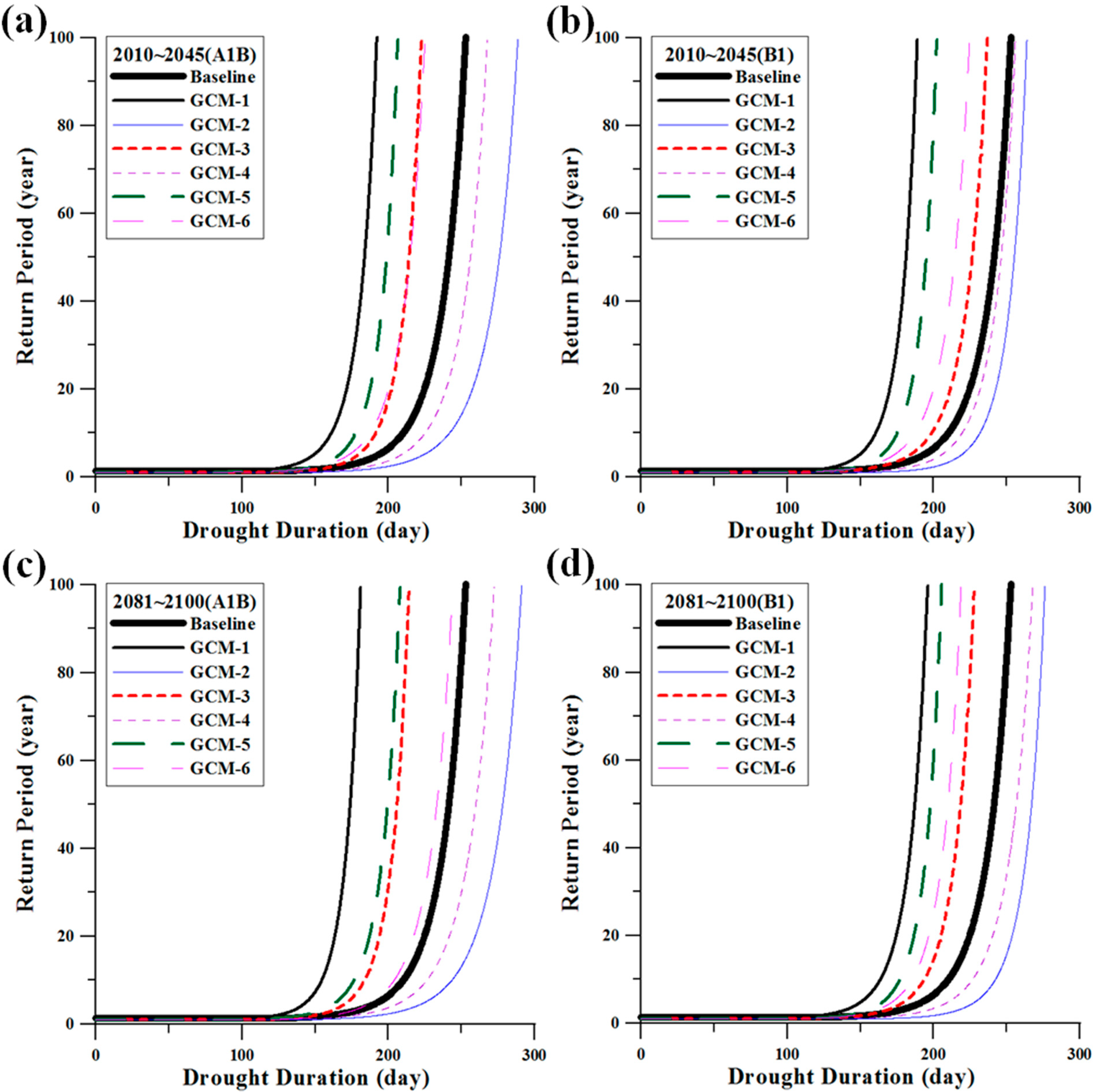
4.4 Drought Frequency Analysis

As an important random phenomenon in hydrology, the frequency analysis is necessary in the aim to know about the drought’s regime. The frequency analysis was performed in the present study for drought duration and magnitude respectively. The estimation steps of the drought frequency analysis are as follows. (1) The annual maximum values of drought duration and magnitude were selected during the baseline and two future periods, respectively; (2) Different probability distributions (including Extreme value type-I, Generalized extreme value, Pearson type-III, Log-Pearson type-III, Three parameters log-normal, Gamma, and Exponential distributions) were used to fit the annual maximum series of drought duration and magnitude, respectively, for each period. This work applied the Kolmogorov-Smirnov test to examine the goodness of fit of the distributions and the root mean square error was used as an index to compare the fitting performances of different distributions; (3) Based on the optimal probability distribution, the drought duration and magnitude with different return periods for a period (baseline or future) can be estimated.

Figure 9. Hydrographs during the dry season. (Thick-solid line: the median during baseline period; Upper and lower thin-solid lines: the 95th and 5th percentiles during baseline period; the same notations are used for scenario data by thick-dash and thin dash lines).

Figure 9. Hydrographs during the dry season. (Thick-solid line: the median during baseline period; Upper and lower thin-solid lines: the 95th and 5th percentiles during baseline period; the same notations are used for scenario data by thick-dash and thin dash lines).

Different probability distributions were tested in the study, and results showed that the Gamma distribution best fits the distributions of drought duration and magnitude. Therefore, the Gamma distribution was used to implement the frequency analysis for drought duration and magnitude respectively. Figure 10 shows the probability distribution of drought duration for each GCM pertaining to two future scenarios and two periods. In the figure, the abscissa indicates the drought duration (day) and the ordinate denotes the return period (year). Results reveal that four GCMs (i.e., GCM-1, GCM-3, GCM-5 and GCM-6) have the same tendency that the drought duration regarding future scenarios will be less than the baseline drought duration for a given return period. However, the other two GCMs (i.e., GCM-2 and GCM-4) have the opposite tendency to the former four GCMs. Therefore, most of GCMs’ results support that there exists a decreasing tendency in drought duration for a given return period; and for a given drought duration, the return period tends to increase which means the occurrence probability of this drought duration tends to decrease.

Figure 11 displays the probability distribution of drought magnitude. In the figure, the abscissa represents the drought magnitude (mm) and the ordinate denotes the return period (year). Results show the drought magnitude of four GCMs (i.e., GCM-1, GCM-3, GCM-5 and GCM-6) in future scenarios have the decreased tendency for a given return period. However, the other two GCMs (i.e., GCM-2 and GCM-4) have the opposite tendency to the former four GCMs. Therefore, most of GCMs’ results support that there exists a decreasing tendency in drought magnitude for a given return period; and for a given drought magnitude, the return period tends to increase which means the occurrence probability of this drought magnitude tends to decrease. From the aforementioned descriptions, most of GCMs’ results support that both the drought duration and magnitude tend to decrease for a given return period in the future, and the occurrence probability of severer drought tends to decrease.

Figure 10. The probability distributions of drought duration for different GCMs, (a) during 2010–2045 under A1B scenario, (b) during 2010–2045 under B1 scenario, (c) during 2081–2100 under A1B scenario, and (d) during 2081–2100 under B1 scenario.

Figure 10. The probability distributions of drought duration for different GCMs, (a) during 2010–2045 under A1B scenario, (b) during 2010–2045 under B1 scenario, (c) during 2081–2100 under A1B scenario, and (d) during 2081–2100 under B1 scenario.

Figure 11. The probability distributions of drought magnitude for different GCMs, (a) during 2010–2045 under A1B scenario, (b) during 2010–2045 under B1 scenario, (c) during 2081–2100 under A1B scenario, and (d) during 2081–2100 under B1 scenario.

Figure 11. The probability distributions of drought magnitude for different GCMs, (a) during 2010–2045 under A1B scenario, (b) during 2010–2045 under B1 scenario, (c) during 2081–2100 under A1B scenario, and (d) during 2081–2100 under B1 scenario.

5. Conclusions and Future Work

This work applied downscaling methods and a hydrological model to derive streamflow under future scenarios and to assess the effect of climate change on streamflow droughts in southern Taiwan. Based on the definition of streamflow drought and the results of ensemble average of the six GCMs used in the present study, it is revealed that scenario droughts may become more frequent, and the duration and magnitude of scenario droughts may become more varied than those of baseline droughts. Analyzing time distributions of streamflow drought under future scenarios found that streamflow drought events will start and end earlier in the future. The streamflow under future scenarios tends to decrease in January and February (at the beginning of paddy rice growth season) but to increase in March and April (at the end of paddy rice growth season). The 90% confidence interval of streamflow under future scenarios is wider than the baseline streamflow after February, because more diverse streamflows are projected. From the frequency analysis, most of GCMs’ results support the streamflow drought duration and magnitude tend to decrease for a given return period in the future, and the occurrence probability of severer drought tends to decrease. Due to the changed pattern of future streamflow drought, the authorities are suggested to plan to moderately adjust irrigation period to adapt to climate change.

From the analytical results of the present study, some future work as the following should be made for reinforcing the study and its conclusions. (1) The combined result of more frequent streamflow drought events and lower duration and magnitude, which is consistent with a change in the temporal variability, is a preliminary conclusion based on the definition of streamflow drought and the results of ensemble average of the six GCMs used in the present study. Future work may adopt more GCMs to analyze the impact of climate change on streamflow droughts to further test this conclusion; (2) The study aimed to investigate the impact of climate change on streamflow droughts. The development and comparisons of downscaling methods were not the main work. Therefore, the downscaling methods used in Taiwan previously were adopted in the present study. Future work may consider the other downscaling approaches (e.g., bias correction methods) for comparing their performances; (3) In Taiwan, the mean flow of a river is about to Q₂₀ (=6.9 mm). Q₅₀ is not a high value during a year. The threshold level method used in the present study is an approach to “define” a streamflow drought for drought studies. The set of threshold level, Q₅₀ and Q₉₀ for the baseline period, was used in the study only for the definition of streamflow drought by which the impact of climate change on this kind of streamflow drought was assessed. The other different sets of threshold level may define different streamflow droughts and can be considered in the future; (4) The study presently considered only three drought indices, i.e., frequency, duration and magnitude, for studying the impact of climate change on streamflow droughts. Since the study area is in the catchment of the reservoir, future work may consider the analysis of operational drought and evaluate other indices that may provide more useful for reservoir management (e.g., the sequent-peak algorithm); (5) In the present study, the parameters of the hydrological model were fixed during both the baseline and future periods. This is because there is no observed data for model calibration during the future period that makes the parameter modification become a big challenge. The fixed parameters for the baseline and future periods made an assumption of the same mechanism of hydrological process in the study area during those periods. Since the study area is small and the catchment characteristics (e.g., the land use, cover, and soil type) in the study area will not obviously change, this assumption can be acceptable. A better way to modify model parameters in the future is suggested to use a fully-physical hydrological model and establish a link between the physical model parameters with climate change; (6) The latest climate change projections are available in the Coupled Model Intercomparison Project Phase 5 (CMIP5). Hence, a further investigation based on these new projections is suggested to include all potential future scenarios for assessing climate change impacts on streamflow drought in the study area.

References

1. Tallaksen, L.M.; van Lanen, H.A.J. Hydrological Drought: Processes and Estimation Methods for Streamflow and Groundwater; Elsevier B.V.: Amsterdam, The Netherlands, 2004. [Google Scholar]
2. Yu, P.S.; Yang, T.C.; Kuo, C.C. Evaluating long-term trends in annual and seasonal precipitation in Taiwan. Water Resour. Manag. 2006, 20, 1007–1023. [Google Scholar] [CrossRef]
3. Chen, S.T.; Kuo, C.C.; Yu, P.S. Historical trends and variability of meteorological droughts in Taiwan. Hydrol. Sci. J. 2009, 54, 430–441. [Google Scholar] [CrossRef]
4. Yevjevich, V. An Objective Approach to Definition and Investigations of Continental Hydrologic Droughts; Hydrology Paper No. 23; Colorado State University: Fort Collins, CO, USA, 1967. [Google Scholar]
5. Burke, E.J.; Perry, R.H.J.; Brown, S.J. An extreme value analysis of UK drought and projections of change in the future. J. Hydrol. 2010, 388, 131–143. [Google Scholar] [CrossRef]
6. Fowler, H.J.; Blenkinsop, S.; Tebaldi, C. Review linking climate change modeling to impacts studies: Recent advances in downscaling techniques for hydrological modeling. Int. J. Climatol. 2007, 27, 1547–1578. [Google Scholar]
7. Wilby, R.L.; Wigley, T.M.L. Downscaling general circulation model output: A review of methods and limitations. Progress Phys. Geogr. 1997, 21, 530–548. [Google Scholar] [CrossRef]
8. Chen, S.T.; Yu, P.S.; Tang, Y.H. Statistical downscaling of daily precipitation using support vector machines and multivariate analysis. J. Hydrol. 2010, 385, 13–22. [Google Scholar]
9. Chu, J.L.; Kang, H.; Tam, C.Y.; Park, C.K.; Chen, C.T. Seasonal forecast for local precipitation over northern Taiwan using statistical downscaling. J. Geophys. Res. 2008, 113, D12118. [Google Scholar]
10. Lin, S.H.; Liu, C.M.; Huang, W.C.; Lin, S.S.; Yen, T.H.; Wang, H.R.; Kuo, J.T.; Lee, Y.C. Developing a yearly warning index to assess the climatic impact on the water resources of Taiwan, a complex–terrain island. J. Hydrol. 2010, 390, 13–22. [Google Scholar] [CrossRef]
11. Yu, P.S.; Yang, T.C. Fuzzy multi-objective function for rainfall-runoff model calibration. J. Hydrol. 2000, 238, 1–14. [Google Scholar] [CrossRef]
12. Yu, P.S.; Yang, T.C.; Wu, C.K. Impact of climate change on water resources in southern Taiwan. J. Hydrol. 2002, 260, 161–175. [Google Scholar] [CrossRef]
13. Bergström, S. Development and Application of a Conceptual Runoff Model for Scandinavian Catchments; SMHI Norrköping: Norrköping, Sweden, 1976. [Google Scholar]
14. Bergström, S. The HBV Model—Its Structure and Applications; SMHI Norrköping: Norrköping, Sweden, 1992. [Google Scholar]
15. Bathia, P.K.; Bergström, S.; Persson, M. Application of the Distributed HBV-6 Model to the Upper Narmada Basin in India; SMHI Norrköping: Norrköping, Sweden, 1984. [Google Scholar]
16. Häggström, M.; Lindström, G.; Cobos, C.; Martinez, J.R.; Merlos, L.; Alonzo, R.D.; Castillo, G.; Sirias, C.; Miranda, D.; Granados, J.I.; et al. Application of the HBV Model for Flood Forecasting in Six Central American Rivers; SMHI Norrköping: Norrköping, Sweden, 1990. [Google Scholar]
17. Bergström, S.; Carlsson, B.; Gardelin, M.; Lindström, G.; Pettersson, A.; Rummukainen, M. Climate change impacts on runoff in Sweden—Assessments by global climate models, dynamical downscaling and hydrological modeling. Clim. Res. 2001, 16, 101–112. [Google Scholar] [CrossRef]
18. Menzel, L.; Bürger, G. Climate change scenarios and runoff response in the Mulde catchment (Southern Elbe, Germany). J. Hydrol. 2002, 267, 53–64. [Google Scholar] [CrossRef]
19. Dibike, Y.B.; Coulibaly, P. Hydrologic impact of climate change in the Saguenay watershed: Comparison of downscaling methods and hydrologic models. J. Hydrol. 2005, 307, 145–163. [Google Scholar] [CrossRef]
20. Yu, P.S.; Wang, Y.C. Impact of climate change on hydrological processes over a basin scale in northern Taiwan. Hydrol. Process. 2009, 23, 3556–3568. [Google Scholar] [CrossRef]
21. IPCC. Climate Change 2007—The Physical science Basis; Fourth Assessment Report of the Intergovernmental Panel on Climate Change; Cambridge University Press: Cambridge, UK, 2007. [Google Scholar]
22. Caron, L.P.; Jones, C.G. Analysing present, past and future tropical cyclone activity as inferred from an ensemble of coupled global climate models. Tellus 2008, 60A, 80–96. [Google Scholar]
23. Min, S.K.; Park, E.H.; Kwon, W.T. Future projections of East Asian climate change from multi—AOGCM ensembles of IPCC SRES scenario simulations. J. Meteorol. Soc. Jpn. 2004, 82, 1187–1211. [Google Scholar] [CrossRef]
24. Kitoh, A.; Uchiyama, T. Changes in onset and withdrawal of the East Asian summer rainy season by multi-model global warming experiments. J. Meteorol. Soc. Jpn. 2006, 84, 247–258. [Google Scholar] [CrossRef]
25. Kim, M.K.; Kang, I.S.; Park, C.K.; Kim, K.M. Superensemble prediction of regional precipitation over Korea. Int. J. Climatol. 2004, 24, 777–790. [Google Scholar] [CrossRef]
26. Feddersen, H.; Andersen, U. A method for statistical downscaling of seasonal ensemble predictions. Tellus 2005, 57A, 398–408. [Google Scholar] [CrossRef]
27. Richardson, C.W. Stochastic simulation of daily precipitation, temperature, and solar radiation. Water Resour. Res. 1981, 17, 182–190. [Google Scholar] [CrossRef]
28. Selker, J.S.; Haith, D.A. Development and testing of single-parameter precipitation distributions. Water Resour. Res. 1990, 26, 2733–2740. [Google Scholar] [CrossRef]
29. Tung, C.P.; Haith, D.A. Global-warming effects on New York streamflows. J. Water Resour. Plan. Manag. 1995, 121, 216–225. [Google Scholar] [CrossRef]
30. Coe, R.; Stern, R.D. Fitting models to rainfall data. J. Appl. Meteorol. 1982, 21, 1024–1031. [Google Scholar]
31. Woolhiser, D.A.; Roldan, J. Stochastic daily precipitation models: 2. A comparison of distribution of amounts. Water Resour. Res. 1982, 18, 1461–1468. [Google Scholar]
32. Schubert, S. A weather generator based on the European “Grosswetterlagen”. Clim. Res. 1994, 4, 191–202. [Google Scholar] [CrossRef]
33. Corte-Real, J.; Xu, H.; Qian, B. A weather generator for obtaining daily precipitation scenarios based on circulation patterns. Clim. Res. 1999, 13, 61–75. [Google Scholar] [CrossRef]
34. Woolhiser, D.A.; Pegram, G.G.S. Maximum likelihood estimation of Fourier coefficients to describe seasonal variation of parameters in stochastic daily precipitation models. J. Appl. Meteorol. 1979, 18, 34–42. [Google Scholar]
35. Woolhiser, D.A.; Roldan, J. Seasonal and regional variability of parameters for stochastic daily precipitation models. Water Resour. Res. 1986, 22, 965–978. [Google Scholar] [CrossRef]
36. Hamon, W.R. Estimating potential evapotranspiration. J. Hydraul. Div. Proc. Am. Soc. Civil Eng. 1961, 871, 107–120. [Google Scholar]
37. Tate, E.L.; Gustard, A. Drought definition: A hydrological perspective. In Drought and Drought Mitigation in Europe; Vogt, J.V., Somma, F., Eds.; Kluwer Academic Publishers: Derdrecht, The Netherlands, 2000; pp. 23–48. [Google Scholar]
38. Kjeldsen, T.R.; Lundorf, A.; Rosbjerg, D. Use of a two-component exponential distribution in partial duration modeling of hydrological droughts in Zimbabwean rivers. Hydrol. Sci. J. 2000, 45, 285–298. [Google Scholar] [CrossRef]
39. Shiau, J.T.; Shen, H.W. Recurrence analysis of hydrological droughts of differing severity. J. Water Resour. Plan. Manag. 2001, 127, 30–40. [Google Scholar] [CrossRef]
40. Hisdal, H.; Stahl, K.; Tallaksen, L.M.; Demuth, S. Have streamflow droughts in Europe become more severe and frequent. Int. J. Climatol. 2001, 21, 317–333. [Google Scholar] [CrossRef]
41. Shiau, J.T. Return period of bivariate distributed extreme hydrological events. Stoch. Environ. Res. Risk Assess. 2003, 17, 42–57. [Google Scholar] [CrossRef]
42. Fleig, A.K.; Tallaksen, L.M.; Hisdal, H.; Demuth, S. A global evaluation of streamflow drought characteristics. Hydrol. Earth Syst. Sci. 2006, 10, 535–552. [Google Scholar] [CrossRef]
43. Shukla, S.; Wood, A.W. Use of a standardized runoff index for characterizing hydrologic drought. Geophys. Res. Lett. 2008, 35, L02405. [Google Scholar] [CrossRef]
44. Tallaksen, L.M. Streamflow drought frequency analysis. In Drought and Drought Mitigation in Europe; Vogt, J.V., Somma, F., Eds.; Kluwer Academic Publishers: Derdrecht, The Netherlands, 2000; pp. 103–117. [Google Scholar]
45. Chu, J.L.; Yu, P.S. A study of the impact of climate change on local precipitation using statistical downscaling. J. Geophys. Res. 2010, 115, D10105. [Google Scholar]
46. Gerrity, J.P. A note on Gandin and Murphy’s equitable skill score. Mon. Weather Rev. 1992, 120, 2709–2712. [Google Scholar]
47. World Meteorological Organization. Standardized Verification System (SVS) for Long-Range Forecasts (LRF); World Meteorological Organization: Geneva, Switzerland, 2002. [Google Scholar]
48. Duan, Q.; Sorooshian, S.; Gupta, V.K. Optimal use of the SCE-UA global optimisation method for calibrating watershed models. J. Hydrol. 1994, 158, 265–284. [Google Scholar] [CrossRef]