Using the Entire Yield Curve in Forecasting Output and Inflation

1
Aarhus University and CREATES, Fuglesangs Allé 4, 8210 Aarhus V, Denmark
2
ICBC Credit Suisse Asset Management, Beijing 100033, China
3
Department of Economics, University of California, Riverside, CA 92521, USA
4
Monetary and Financial Market Analysis Section, Division of Monetary Affairs, Federal Reserve Board, Washington, DC 20551, USA
*
Author to whom correspondence should be addressed.
Econometrics 2018, 6(3), 40; https://doi.org/10.3390/econometrics6030040
Submission received: 17 June 2018
/
Revised: 17 August 2018
/
Accepted: 21 August 2018
/
Published: 29 August 2018
(This article belongs to the Special Issue Recent Advances in Theory and Methods for the Analysis of High Dimensional and High Frequency Financial Data)
Abstract
:In forecasting a variable (forecast target) using many predictors, a factor model with principal components (PC) is often used. When the predictors are the yield curve (a set of many yields), the Nelson–Siegel (NS) factor model is used in place of the PC factors. These PC or NS factors are combining information (CI) in the predictors (yields). However, these CI factors are not “supervised” for a specific forecast target in that they are constructed by using only the predictors but not using a particular forecast target. In order to “supervise” factors for a forecast target, we follow Chan et al. (1999) and Stock and Watson (2004) to compute PC or NS factors of many forecasts (not of the predictors), with each of the many forecasts being computed using one predictor at a time. These PC or NS factors of forecasts are combining forecasts (CF). The CF factors are supervised for a specific forecast target. We demonstrate the advantage of the supervised CF factor models over the unsupervised CI factor models via simple numerical examples and Monte Carlo simulation. In out-of-sample forecasting of monthly US output growth and inflation, it is found that the CF factor models outperform the CI factor models especially at longer forecast horizons.
Keywords:
level, slope, and curvature of the yield curve; Nelson-Siegel factors; supervised factor models; combining forecasts; principal componentsJEL Classification:
C5; E4; G11. Introduction
The predictive power of the yield curve for macroeconomic variables has been documented in the literature for a long time. Many different points on the yield curve have been used and various methodologies have been examined. For example, Stock and Watson (1989) find that two interest rate spreads, the difference between the six-month commercial paper rate and the six-month Treasury bill rate, and the difference between the ten-year and one-year Treasury bond rates, are good predictors of real activity, thus contributing to their index of leading indicators. Bernanke (1990), Friedman and Kuttner (1993), Estrella and Hardouvelis (1991), and Kozicki (1997), among many others, have investigated a variety of yields and yield spreads individually on their ability to forecast macroeconomic variables. Hamilton and Kim (2002) as well as Diebold et al. (2005) provide a brief summary of this line of research and the link between the yield curve and macroeconomic variables.
Various macroeconomic models for exploring the yield curve information for real activity prediction are proposed. Ang and Piazzesi (2003) and Piazzesi (2005) study the role of macroeconomic variables in an arbitrage-free affine yield curve model. Estrella (2005) constructs an analytical rational expectations model to investigate the reasons for the success of the slope of the yield curve (the spread between long-term and short-term government bond rates) in predicting real economic activity and inflation. The model in Ang et al. (2006), Piazzesi and Wei is an arbitrage-free dynamic model (using lags of GDP growth and yields as regressors) that characterizes expectations of GDP growth. Rudebusch and Wu (2008) provide an example of a macro-finance specification that employs more macroeconomic structure and includes both rational expectations and inertial elements.
Stock and Watson (1999, 2002) investigate forecasts of output growth and inflation using over a hundred of economic indicators, including many interest rates and yield spreads. Stock and Watson (2002, 2012) advocate methods that aim at solving the large-N predictor problem, particularly those using principal components (PC). Ang et al. (2006) suggest the use of the short rate, the five-year to three-month yield spread, and lagged GDP growth in forecasting GDP growth out-of-sample. The choice of these two yield curve characteristics, as they argue, is because they have almost one-to-one correspondence with the first two principal components of the short rate and five yield spreads that account for of quarterly yield curve variation.
Alternatively to the PC factor approach on the large-N predictor information set, Diebold and Li (2006) propose the Nelson and Siegel (1987) (NS) factors for the large-N yields. They use a modified three-factor NS model to capture the dynamics of the yield curve and show that the three NS factors may be interpreted as level, slope, and curvature. Diebold et al. (2006) examine the correlations between NS yield factors and macroeconomic variables. They find that the level factor is highly correlated with inflation and that the slope factor is highly correlated with real activity. For more on the yield curve background and the three characteristics of the yield curve, see Litterman and Scheinkman (1991) and Diebold and Li (2006).
In this paper, we utilize the yield curve information for prediction of macro-economic variables. Using a large number of yield curve points with different maturities yields a large-N problem in the predictive regression. The PC factors or the NS factors of the yield curve may be used to reduce the large dimension of the predictors. However, the PC and NS factors of the yield curve are not supervised for a specific variable to forecast. These factors simply combine information (CI) of many predictors (yields) without having to look at a forecast target. Hence, the conventional CI factor models (using factors of the predictors) are unsupervised for any forecast target.
Our goal in this paper is to consider factor models where the factors are computed with a particular forecast target in mind. Specifically, we consider the PC or NS factors of forecasts (not of predictors), with each of the forecasts formed using one predictor at a time. (It could be generalized to make each forecast from using more than one predictor, e.g., a subset of the N predictors, in which case there can be as many as forecasts to combine.) These factors will combine the forecasts (CF). The PC factors of forecasts are combined forecasts using the combining weights that solves a singular value problem for a set of forecasts, while the NS factors of forecasts are combined forecasts using the combining weights obtained from orthogornal polynomials that emulate the shape of a yield curve (in level, slope, and curvature). The PC or NS factors of the many forecasts are supervised for a forecasting target. The main idea of the CF-factor model is to focus on the space spanned by forecasts rather than the space spanned by predictors. The factorization of forecasts (CF-factor model) can substantially improve forecasting performance compared to the factorization of predictors (CI-factor model). This is because the CF-factor model takes the forecast target into the factorization, while the conventional CI-factor model is blind to the forecast target because the factorization uses only information on predictors.
For both CI and CF schemes, the NS factor model can be relevant only when the yield curve is used as predictors while the PC factor model can be used in general. The NS factors are specific to the yield curve factors such as level, slope, and curvature factors. When the predictors are from the points on the yield curve, the NS factor models proposed here is nearly the same as the PC factors. Given the similarity of NS and PC and the generality of PC, we begin the paper with the PC models to understand the mechanism of the supervision in CF-factor models. We demonstrate how the supervised CF factor models outperform the unsupervised CI factor model, under the presence of many predictors (50 points on the yield curve at each time). The empirical work shows that there are potentially big gains in the CF-factor models. In out-of-sample forecasting of U.S. monthly output growth and inflation, it is found that the CF factor models (CF-NS and CF-PC) are substantially better than the conventional CI factors models (CI-NS and CI-PC). The advantage of supervised factors is even greater for longer forecast horizons.
The paper is organized as follows: in Section 2, we describe the CI and CF frameworks and principal component approaches for their estimation, present theoretical results about supervision, and an example to provide intuition. Section 3 provides simulations of supervision under different noise, predictor correlation, and predictor persistence conditions. In Section 4, we introduce the NS component approaches for the CI and CF frameworks. In Section 5, we show the out-of-sample performance of the proposed methods in forecasting U.S. monthly output growth and inflation. Section 6 presents the conclusions.
2. Supervising Factors
2.1. Factor Models
Let denote the variable to be forecast (output growth or inflation) using yield curve information stamped at time t, where h denotes the forecast horizon. The predictor vector contains information about the yield curve at various maturities: , where denotes the yield at time t with maturity .
Consider the CI model when N is large
for which the forecast at time T is
with estimated by OLS using the information up to time T. A problem is that here the mean-squared forecast error (MSFE) is of order increasing with 1 A solution to this problem is to reduce the dimension either by selecting a subset of the N predictors, e.g., by Lasso type regression (Tibshirani 1996) or by using factor models of, e.g., Stock and Watson (2002). In this paper, we focus on using the factor model rather than selecting a subset of the N predictors.2
2.1.1. CI-Factor Model
The conventional factor model is the CI factor model for of the form
where is and is The estimated factor loadings are obtained either by following Stock and Watson (2002) and Bai (2003), or by following Nelson and Siegel (1987) and Diebold and Li (2006). The latter approach is discussed in Section 4. The factors are then estimated by
As this model computes the factors from all N predictors of directly, it will be called “CI-factor”. The forecast can be formed using estimated at time T from the regression
In matrix form, we write the factor model (3) and (5) for the vector of forecast target observations y and for the matrix of predictors X as follows:3
where y is the vector of observations, is a matrix of factors, is an matrix of factor loadings, is a parameter vector, is a random matrix, and is a vector of random errors.
Remark 1. (No supervision in CI-factor model):
Consider the joint density of
where is the conditional density of given and is the marginal density of . The CI-factor model assumes a situation where the joint density operates a “cut” in the terminology of Barndorff-Nielsen (1978) and Engle et al. (1983), such that
where and are “variation-free”. Under this situation, the forecasting equation in (5) is obtained from the conditional model and the factor equation in (3) is solely obtained from the marginal model of the predictors. The computation of the factors is entirely from the marginal model that is blind to the forecast target
While the CI factor analysis of a large predictor matrix X solves the dimensionality problem, it computes the factors using information in X only, without accounting for the variable y to be forecast, and therefore the factors are not supervised for the forecast target. Our goal in this paper is to improve this approach by accounting for the forecast target in the computation of the factors. The procedure will be called supervision.
There are some attempts in the literature to supervise factor computation for a given forecast target. For example, Bair et al. (2006) and Bai and Ng (2008) consider factors of selected predictors that are informative for a specified forecast target; Zou et al. (2006) consider sparse loadings of principal components; De Jong (1993) and Groen and Kapetanios (2016) consider partial least squares regression; De Jong and Kiers (1992) consider principal covariate regression; Armah and Swanson (2010) select variables for factor proxies that have the maximum predictive power for the variable being forecast; and some weighted principal components have been used to downweight noisier series.
In this paper, we consider the CF-factor model that computes factors from forecasts rather than from predictors. This approach has been proposed in Chan et al. (1999) and in Stock and Watson (2004), there labeled “principal component forecast combination”. We will refer to this approach as CF-PC (combining forecasts principal components). The details are as follows.
2.1.2. CF-Factor Model
The forecasts from a CF-factor model are computed in two steps. The first step is to estimate the factors of the individual forecasts. Let the individual forecasts be formed by regressing the forecast target using the ith individual predictor :
Stack the N individual forecasts into a vector and consider a factor model of :
The CF-factor is estimated from
The second step is to estimate the forecasting equation (for which the estimated CF-factors from the first step are used as regressors)4
Then, the CF-factor forecast at time T is
where is estimated. See (Chan et al. 1999; Huang and Lee 2010; Stock and Watson 2004).
To write the CF-factor model in matrix form, we assume for notational simplicity that the data has been centered so that we do not include a constant term. We regress y on the columns of X, , one at a time, and write the fitted values in (10) as
Collect the fitted values in the matrix
where is a diagonal matrix containing the regression coefficients. We call B the supervision matrix. Then, the CF-factor model is
where is a matrix of factors of , is an matrix of factor loadings, is an parameter vector, is a random matrix, and is a vector of random errors. In the rest of the paper, the subscripts CI and CF may be omitted for simplicity.
We use principal components (PC) as discussed in Stock and Watson (2002), Bai (2003), and Bai and Ng (2006). For the specific case of yield curve data, we use NS components as discussed in Nelson and Siegel (1987) and Diebold and Li (2006). We use both CF and CI approaches together with PC factors and NS factors. Our goal is to show that forecasts using supervised factor models (CF-PC and CF-NS) are better than forecasts from conventional unsupervised factor models (CI-PC and CI-NS). We show analytically and in simulations how supervision works to improve factor computation with respect to a specified forecast target. In Section 5, we present empirical evidence.
Remark 2. (Estimation of B):
The CF-factor model in (17) and (18) with (identity matrix) is a special case when there is no supervision. In this case, the CF-factor model collapses to the CI-factor model. If B were consistently estimated by minimizing the forecast error loss, then the CF-factor model with the “optimal” B would outperform the CI-factor model. However, as the dimension of the supervision matrix B grows with , B is an “incidental parameter” matrix and can not be estimated consistently. See Neyman and Scott (1948) and Lancaster (2000). Any estimation error in B translates into forecast error in the CF-factor model. Whether there is any virtue in considering Bayesian methods of estimating B, while still avoiding this problem, is left for future research. Instead, in this paper, we circumvent this difficulty by imposing that be a diagonal matrix and by estimating the diagonal elements ’s from the ordinary least squares regression in (10) or (15) with one predictor at a time. The supervision matrix B can be non-diagonal in general. As imposing the diagonality on B may be restrictive, it would be an interesting empirical question to examine if the CF-factor forecast with this restriction and the estimation strategy of B can still outperform the CI-factor forecast with Our empirical results in Section 5 (Table 1) support this simple estimation strategy for the diagonal matrix in favor of the CF-factor model.
Remark 3. (Combining forecasts with many predictors):
It is generally believed that it is difficult to estimate the forecast combination weights when N is large. Therefore, the equal weights have been widely used instead of estimating weights.5It is often found in the literature that equally-weighted combined forecasts are often the best. Stock and Watson (2004) call this the “forecast combination puzzle”. See also Timmermann (2006). Smith and Wallis (2009) explore a possible explanation of the forecast combination puzzle and conclude that it is due to estimation error of the combining weights.
2.2. Singular Value Decomposition
In this section, we formalize the concept of supervision and explain how it improves factor extraction. We compare the two different approaches CI-PC (Combining Information—Principal Components) and CF-PC (Combining Forecasts—Principal Components) in a linear forecast problem of the time series y given predictor data X. We explain the advantage of the CF-PC approach over CI-PC in Section 2.3 and give some examples in Section 2.4. We explore the advantage of supervision in simulations in Section 3.2. As an alternative to PC factors, we propose the use of NS factors in Section 4.
Principal components of predictorsX(CI-PC): Let be a matrix of regressors and let
be the singular value decomposition of X, with diagonal rectangular, that is, diagonal square matrix padded with zero rows below the square if or padded with zero columns next to the square if , , and is unitary. Write
where is diagonal and square. Therefore, W contains the eigenvectors of . For a matrix , denote by the matrix consisting of the first columns of A. Then, is the matrix containing the singular vectors corresponding to the largest singular values . The first k principal components are given by
where is the identity matrix, is an matrix of zeros, and is the upper-left diagonal block of . Note that the first k principal components of X are constant multiples of columns of as is diagonal. The projection (forecast) of y onto is given by
as . Therefore, the CI forecast, is the projection of y onto The CI forecast error and the CI sum of squared error (SSE) are
as is symmetric idempotent.
Bai (2003) shows that, under general assumptions on the factor and error structure, is a consistent and asymptotically normal estimator of , where H is an invertible matrix.6 This identification problem is also clear from Equation (24), and it conveniently allows us to identify the principal components as since is diagonal. The principal components are scalar multiples of the first k columns of Bai’s result shows that principal components can be estimated consistently only up to linear combinations. Bai and Ng (2006) show that the parameter vector in the forecast equation can be estimated consistently for with an asymptotically normal distribution.
Principal components of forecasts (CF-PC): To generate forecasts in a CF-factor scheme, we regress y on the columns of X, , one at a time, and calculate the fitted values of (15). Collect the fitted values in the matrix as in (16), with containing the regression coefficients in its diagonal. Compute the singular value decomposition of :
with is diagonal rectangular, and unitary. Pick the first principal components of ,
where is the matrix of the singular vectors corresponding to the k largest singular values and is the upper-left diagonal block of Again, we can identify the estimated k principal components of with , where is the matrix of factors of . The projection (forecast) of y onto is given by:
as . The CF forecast, is the projection of y onto The CF forecast error and the CF SSE are
as is symmetric idempotent.
2.3. Supervision
In this sub-section, we explain the advantage of CF-PC over CI-PC in factor computation. We call the advantage “supervision”, which is defined as follows:
Definition 1.
(Supervision). The advantage of CF-PC over CI-PC, called supervision, is the selection of principal components according to their contribution to variation in y, as opposed to selection of principal components according to their contribution to variation in the columns of X. This is achieved by selecting principal components from a matrix of forecasts of y.
We use the following measures of supervision of CF-PC in comparison with CI-PC.
Definition 2.
(Absolute Supervision). Absolute supervision is the difference of the sums of squared errors (SSE) of CI-PC and CF-PC:
Definition 3.
(Relative Supervision). Relative supervision is the ratio of the sums of squared errors of CI-PC over CF-PC:
Remark 4.
When , there is no room for supervision
because Relative supervision is defined only for
For the sake of simplifying the notation and presentation, we consider the same number of factors in CI and CF factor models with for the rest of the paper.
Remark 5.
is a block of a basis change matrix that in the expression returns the first k coordinates of y with respect to the new basis. This new basis is the one with respect to which the mapping becomes diagonal, with singular values in descending order such that the first k columns of S correspond to the k largest singular values. Therefore, is the sum of the squares of these coordinates. Broadly speaking, the are the k largest components of y in the sense of and its construction from the single regression coefficients. Thus, is the sum of the squares of the k coefficients in y that contributes most to the variation in the columns of .
Analogously, is a block of a basis change matrix that for returns the first k coordinates of y with respect to the basis that diagonalizes the mapping . Therefore, is the sum of squares of the k coordinates of y selected according to their contribution to variation in the columns of X.
We emphasize the factors that explain most of the variation of the columns of X, i.e., the eigenvectors associated with the largest eigenvalues of , which are selected in the principal component analysis of X, may have little to do with the factors that explain most of the variation of y, however. The relation between X and y in the data-generating process can, at worst, completely reverse the order of principal components in the columns of X and in y. We demonstrate this in the following Example 1.
2.4. Example 1
In this subsection, we give a small example to facilitate intuition for the supervision mechanics of CF-PC. Example 1 illustrates how the supervision of factor computation defined in Definition 1 operates. In Example 2 in the next section, we add randomness to Example 1 to explore the effect of stochasticity in a well-understood problem.
Let
with and . The singular value decomposition of is
Let
Then, the diagonal matrix B that contains the coefficients of y w.r.t. each column of X is
and
The singular value decomposition of is
We set and compare CI-PC and CF-PC with the same number of principal components. Recall from (23) that and from (28) that . The absolute supervision and relative supervision, defined in (32) and (33), are computed for each
See Appendix A for the calculation. The absolute supervision is all positive and the relative supervision is larger than 1 for all
| k = 1 | 24 | 1.8 |
| k = 2 | 36 | 3.6 |
| k = 3 | 36 | 8.2 |
| k = 4 | 24 | 25.0 |
| k = 5 | 0 | N/A |
As noted in Remarks 1 and 5, the relation between X and y is crucial. In this example, the magnitude of the components in y is reversed from the order in X. For X, the ordering of the columns of X with respect to the largest eigenvalues of is . For y, the ordering of the columns of X with respect to the largest eigenvalues of is . For example, consider the case , i.e., we choose two out of five factors in the principal component analysis. CI-PC, the analysis of X, will pick the columns 3 and 1 of X, that is, the vectors and . These correspond to the two largest singular values 1 and of X. CF-PC, the analysis of , will pick columns 4 and 5 of X, that is, the vectors and . These correspond to the two largest singular values 5 and 4 of . The regression coefficients in de-emphasize columns 3 and 1 of X and emphasize columns 4 and 5 of X.
3. Monte Carlo
There are several simplifications in the construction of Example 1, which we relax by the following extensions:
(a) Adding randomness makes the estimation of the regression coefficients in B a statistical problem. The sampling errors influence the selection of the components of . (b) Adding correlation among regressors (columns of ) introduces correlation among individual forecasts (columns of ), increasing the effect of sampling error in the selection of the components of . (c) Increasing N to realistic magnitudes, in particular in the presence of highly correlated regressors, will increase estimation error in the principal components due to collinearity.
We address the first extension (a) in Example 2. All three extensions (a), (b), (c) are addressed in Example 3 of Section 3.2.
3.1. Example 2
Consider adding some noise to X, y in Example 1. Let v be a matrix of independent random numbers, each entry distributed as , and u be a vector of independent random numbers, each distributed as . In this example, the new regressor matrix X is the sum of X in Example 1 and the noise term v, and the new y is the sum of y in Example 1 and the noise term u. For simplicity, we set in the simulations and let both range from 0.01 to 3. This covers a substantial range of randomness given the magnitude of the numbers in X and y. For each scenario of , we generate 1000 random matrices v and random vectors u and calculate the Monte Carlo average of the sums of squared errors (SSE).
Figure 1 plots the Monte Carlo average of the SSEs for selection of to components. For standard deviations close to zero, the sum of squared errors are as calculated in Example 1. As the noise increases, the advantage of CF over CI decreases but remains substantial, in particular for smaller numbers of principal components. For estimated components (not shown), the SSEs of CI-PC and CF-PC coincide because .
3.2. Example 3
We consider the data-generating process (DGP)
where y is the vector of observations, F is a matrix of factors, is an matrix of factor loadings, is an parameter vector, v is a random matrix, and u is a vector of random errors. We set , and consider data-generating factors.
Note that, under this DGP, the CI-PC model in Equations (6) and (7) is correctly specified if the correct number of factors is identified, i.e., . Even under this DGP, however, an insufficient number of factors, can still result in an advantage of the CF-PC model over the CI-PC model. We will explore this question in this section.
Factors and persistence: For each run in the simulation, we generate the r factors in F as independent AR(1) processes with zero mean and a normally distributed error with mean zero and variance one:
We consider a grid of 19 different AR(1) coefficients , equidistant between 0 and 0.90. We consider data-generating factors and estimated factors.
Contemporaneous factor correlation: Given a correlation coefficient for adjacent regressors, the matrix of factor loadings is obtained from the first r columns of an upper triangular matrix from a Cholesky decomposition of
We consider a grid of 19 different values for , equidistant between the points and . In this setup, the 10th value is very close to . Then, the covariance matrix of the regressors is given by
where and is given by the identity matrix in our simulations. The relation is due to the independence of the factors, but may be subject to substantial finite sample error, in particular for close to one, for well-known reasons.
Relation ofXandy: The parameter vector is drawn randomly from a standard normal distribution for each run in the simulation. This allows to randomly shuffle which factors are important for y.
Noise level: We set and let it range between 0.1 and 3 in steps of 0.1. We add the case of 0.01 that essentially corresponds to a deterministic factor model.
For a given number of data-generating factors, the simulation setup varies along the dimensions (19 points), k (4 points), (19 points), (31 points). For every single scenario, we run 1000 simulations and calculate the SSEs of CI-PC and CF-PC, and the relative supervision . Then, we take the Monte Carlo average of the SSEs and over the 1000 simulations.7
The Monte Carlo results are presented in Figure 2, Figure 3 and Figure 4. Each figure contains four panels that plot the situation for estimated number of factors. The main findings from the figures can be summarized as follows:
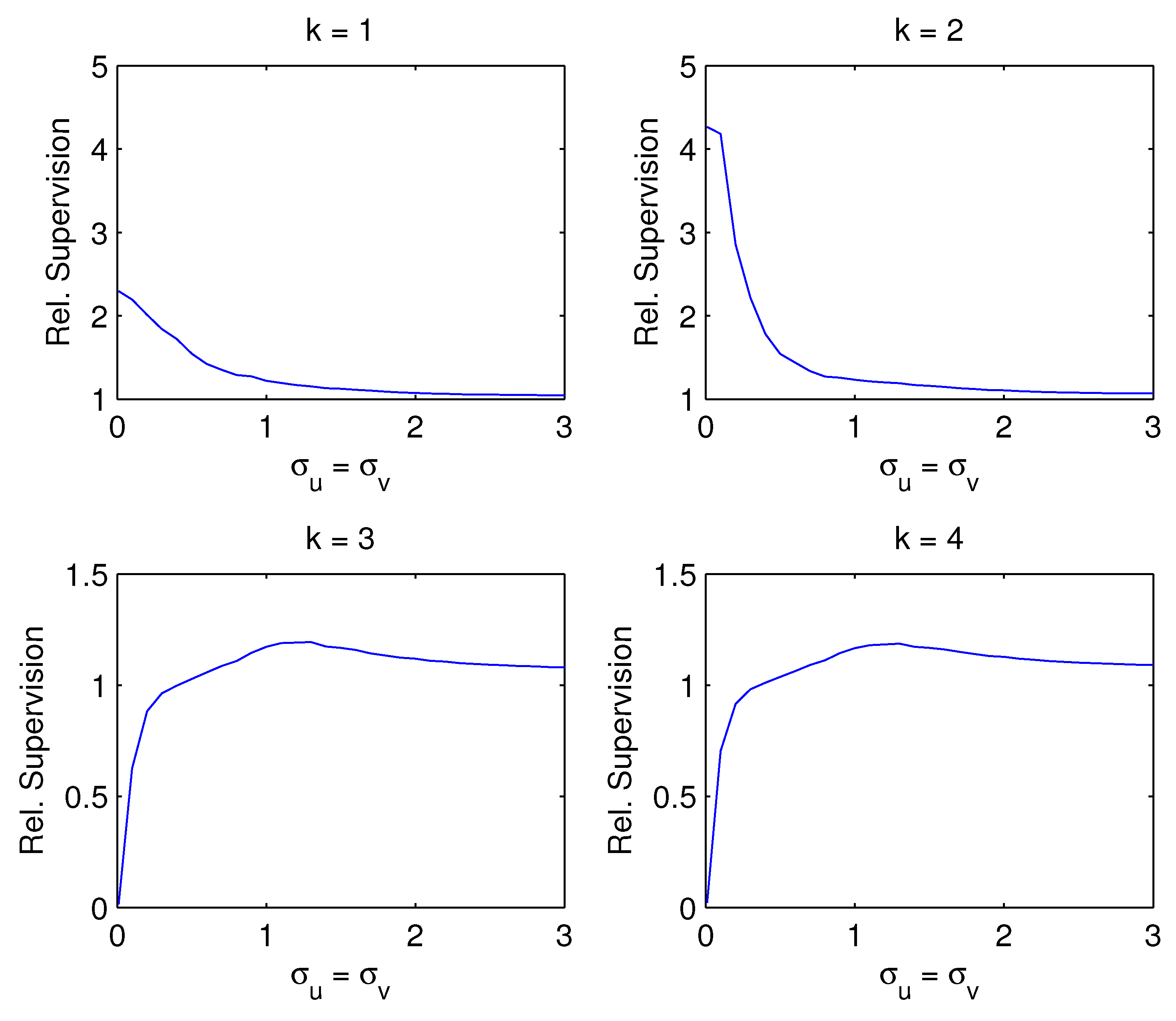
- Figure 2: If the number of estimated factors k is below the true number , as shown in top panels, the supervision becomes smaller with increasing noise. If the correct number of factors or more are estimated as in bottom panels, the advantage of supervision increases with the noise level , Even in this case when the CI-PC is the correct model ( supervision becomes larger as the noise increases.
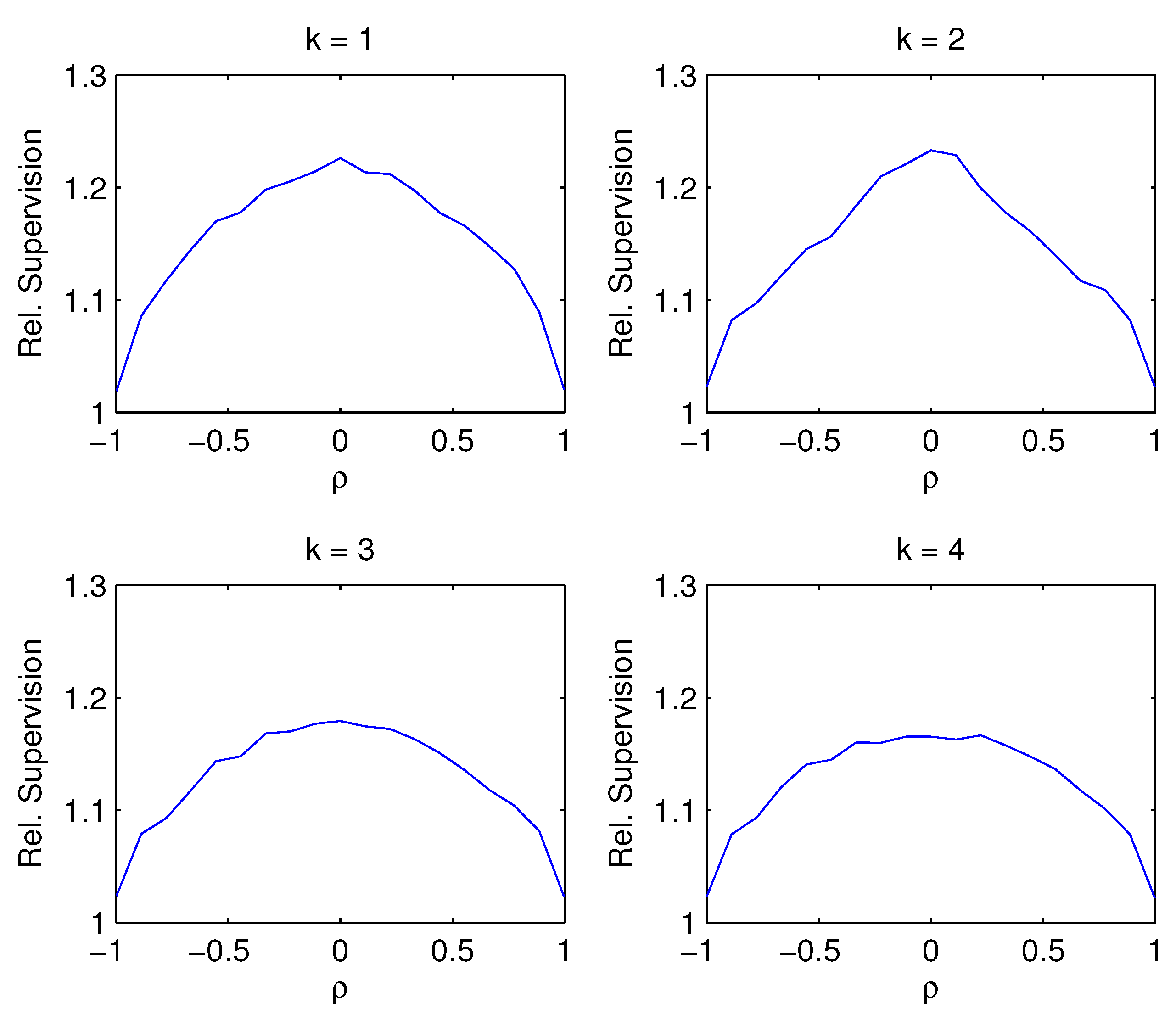
- Figure 3: The advantage of supervision is greatest when the contemporaneous correlation between predictors is minimal. For almost perfect correlation, the advantage of supervision disappears. This is true regardless of whether the correct number of factors is estimated or not. Intuitively, for near-perfect factor correlation, the difference between those factors that explain variation in the columns of X and those that explain variation in vanishes, and so supervision becomes meaningless.
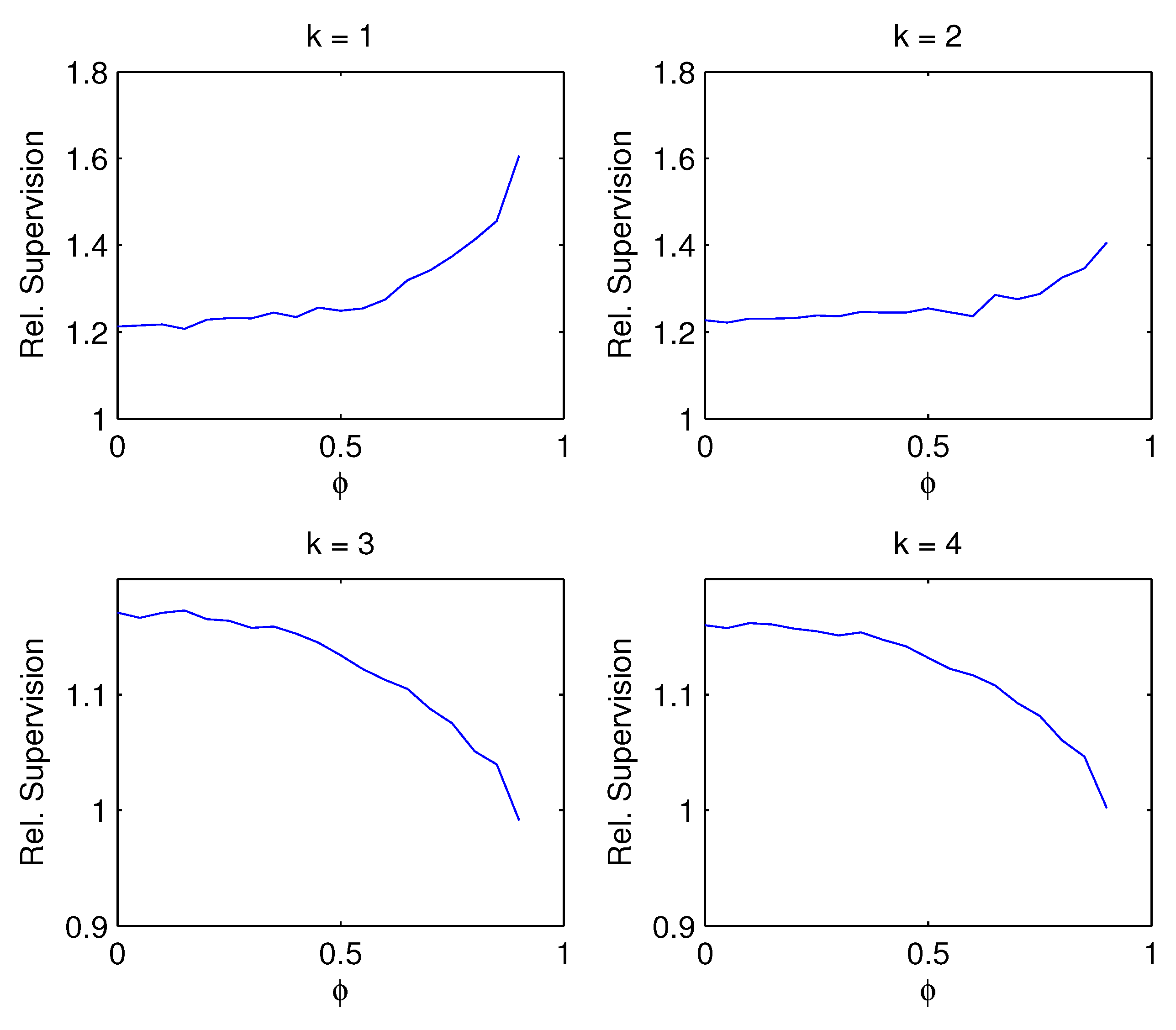
- Figure 4: If the correct number of factors or more are estimated , the advantage of supervision decreases with factor persistence . High persistence induces spurious contemporaneous correlation, and in this sense the situation is related to the result in No. 2. If the number of estimated factors is below the true number of factors , however, the advantage of supervision increases with factor persistence.
4. Supervising Nelson–Siegel Factors
In the previous section, we have examined the factor model based on principal components. When the predictors are points on the yield curve, an alternative factor model can be constructed based on Nelson–Siegel (NS) components. We introduce two new factor models, CF-NS and CI-NS, by replacing principal components with NS components in CF-PC and CI-PC models. Like CI-PC, CI-NS is unsupervised. Like CF-PC, CF-NS is supervised for the particular forecast target of interest.
4.1. Nelson–Siegel Components of the Yield Curve
As an alternative to using principal components in the factor model, one can apply the modified Nelson–Siegel (NS) three-factor framework of Diebold and Li (2006) to factorize the yield curve. Nelson and Siegel (1987) propose Laguerre polynomials with weight function to model the instantaneous nominal forward rate (forward rate curve)
where , , and for all j. The decay parameter may change over time, but we fixed for all t following Diebold and Li (2006).8
Then, the continuously compounded zero-coupon nominal yield of the bond with maturity months at time t is
Allowing the ’s to change over time and adding the approximation error we obtain the following approximate NS factor model for the yield curve for :
where are the three NS factors and are the factor loadings. Because and with (say) is proportional to the three NS factors are associated with level, slope, and curvature of the yield curve.
4.2. CI-NS and CF-NS
4.2.1. NS Components of Predictors X (CI-NS)
We have N predictors of yields where denotes the yield to maturity months at time t, Stacking for (48) can be written as
or
where denotes the i-th row of
which is the matrix of known factor loadings because we fix following Diebold and Li (2006). The NS factors are estimated from regressing on (over by fitting the yield curve period by period for each t.
Then, we consider a linear forecast equation
in order to forecast (such as output growth or inflation). We first estimate using the information up to time T and then form the forecast we call CI-NS by
This method is comparable to CI-PC with number of factors fixed at . It differs from CI-PC, however, in that the three NS factors have intuitive interpretations as level, slope and curvature of the yield curve, while the first three principal components may not have a clear interpretation. In the empirical section, we also consider two alternative CI-NS forecasts by including only the level factor (denoted CI-NS (, and only the level and slope factors (denoted CI-NS ()) to see whether the level factor or the combination of level and slope factors have dominant contribution in forecasting output growth and inflation.
4.2.2. NS Components of Forecasts (CF-NS)
While CI-NS solves the large-N dimensionality problem by reducing the N yields to three factors , it computes the factors entirely from yield curve information only, without accounting for the variable to be forecast. Similar in spirit to CF-PC, here we can improve CI-NS by supervising the factor computation, which we term as CF-NS.
The CF-NS forecast is based on the NS factors of , a vector of the N individual forecasts as in (10) and (11),
with in (51). Hence, for the NS factor models. Note that, when the NS factors loadings are normalized to sum up to one, the three CF-NS factors
are weighted individual forecasts with the three normalized NS loadings, with , , and . The CF-NS forecast can be obtained from the forecasting equation
which is denoted CF-NS. The parameter vector is estimated using information up to time T. Using only the first factor or the first two factors, one can obtain the forecasts CF-NS and CF-NS
Note that, while the CF-PC method can be used for data of many kinds, the CF-NS method we propose is tailored to forecasting using the yield curve. It uses fixed factor loadings in that are the NS exponential factor loadings for yield curve modeling, and hence avoids the estimation of factor loadings. In contrast, CF-PC needs to estimate .
Also note that, by construction, CF-NS is the equally weighted combined forecast .
5. Forecasting Output Growth and Inflation
This section presents the empirical analysis where we describe the data, implement forecasting methods introduced in the previous sections on forecasting output growth and inflation, and analyze out-of-sample forecasting performances. This allows us to analyze the differences between output growth and inflation forecasting using the same yield curve information and to compare the strengths of different methods.
5.1. Data
Let denote the variable to be forecast (output growth or inflation) using yield information up to time t, where h denotes the forecast horizon. The predictor vector contains the information about the yield curve at various maturities: denotes the zero coupon yield of maturity months at time t.
Two forecast targets, output growth and inflation, are constructed respectively as monthly growth rate of Personal Income (PI, seasonally adjusted annual rate) and monthly change in CPI (Consumer Price Index for all urban consumers: all items, seasonally adjusted) from 1970:01 to 2010:01. PI and CPI data are obtained from the web site of the Federal Reserve Bank of St. Louis (FRED2).
We apply the following data transformations. For the monthly growth rate of PI, we set as the forecast target (as used in Ang et al. (2006)). For the consumer price index (CPI), we set as the forecast target (as used in Stock and Watson (2007)).9
Our yield curve data consist of U.S. government bond prices, coupon rates, and coupon structures, as well as issue and redemption dates from 1970:01 to 2009:12.10 We calculate zero-coupon bond yields using the unsmoothed Fama and Bliss (1987) approach. We measure bond yields on the second day of each month. We also apply several data filters designed to enhance data quality and focus attention on maturities with good liquidity. First, we exclude floating rate bonds, callable bonds and bonds extended beyond the original redemption date. Second, we exclude outlying bond prices less than 50 or greater than 130 because their price discounts/premium are too high and imply thin trading, and we exclude yields that differ greatly from yields at nearby maturities. Finally, we use only bonds with maturity greater than one month and less than fifteen years because other bonds are not actively traded. Indeed, to simplify our subsequent estimation, using linear interpolation we pool the bond yields into fixed maturities of 1, 2, 3, 4, 5, 6, 7, 8, 9, 10, 11, 12, 13, 14, 15, 16, 17, 18, 19, 20, 21, 22, 23, 24, 25, 26, 27, 28, 29, 30, 33, 36, 39, 42, 45, 48, 51, 54, 57, 60, 63, 66, 72, 78, 84, 90, 96, 102, 108, and 120 months, where a month is defined as 30.4375 days.11
We examine some descriptive statistics (not reported for space) of the two forecast targets and yield curve level, slope, and curvature (empirical measures), over the full sample from 1970:01 to 2009:12 and the out-of-sample evaluation period from 1995:02 to 2010:01. We observe that both PI growth and CPI inflation become more moderate and less volatile from around the mid-1980s. This has become a stylized fact known as the “Great Moderation”. In particular, there is a substantial drop in persistency of CPI inflation. The volatility and persistency of the yield curve slope and curvature do not change much. The yield curve level, however, decreases and stabilizes.
In predicting macroeconomic variables using the term structure, yield spreads between yields with various maturities and the short rate are commonly used in the literature. One possible reason for this practice is that yield levels are treated as I(1) processes, so yield spreads will likely be I(0). Similarly, macroeconomic variables are typically assumed to be I(1) and transformed properly into I(0), so that, in using yield spreads to forecast macro targets, issues such as spurious regression are avoided. In this paper, however, we use yield levels (not spreads) to predict PI growth and CPI inflation (not change in inflation), for the following reasons. First, whether yields and inflation are I(1) or I(0) is still arguable. Stock and Watson (1999, 2012) use yield spreads and treat inflation as I(1), so they forecast change in inflation. Inoue and Kilian (2008), however, treat inflation as I(0). Since our target is forecasting inflation, not change in inflation, we will treat CPI inflation as well as yields as I(0) in our empirical analysis. Second, we emphasize real-time, out-of-sample forecasting performance more than in-sample concerns. As long as out-of-sample forecast performance is unaltered or even improved, we think the choice of treating the variables as I(1) or I(0) variables does not matter much.12 Third, using yield levels will allow us to provide clearer interpretations for questions such as what part of the yield curve contributes the most towards predicting PI growth or CPI inflation, and how the different parts of the yield curve interact in the prediction, etc.
5.2. Out-of-Sample Forecasting
All forecasting models are estimated in a rolling window scheme with window size months ending at month t (starting at ). In the evaluation period from 1995:02 to 2010:01 (180 months), the first rolling sample to estimate models begins at 1970:02 and ends at 1995:01, the second rolling sample is for 1970:03–1995:02, the third 1970:04–1995:03, and so on. The out-of-sample evaluation period is from 1995:02 to 2010:01 (hence out-of-sample size ).13 In all NS-related methods (CI and CF), we set , the parameter that governs the exponential decay rate, at for reasons discussed in Diebold and Li (2006).14 We compare h-months-ahead out-of-sample forecasting results of those methods introduced so far for months ahead.
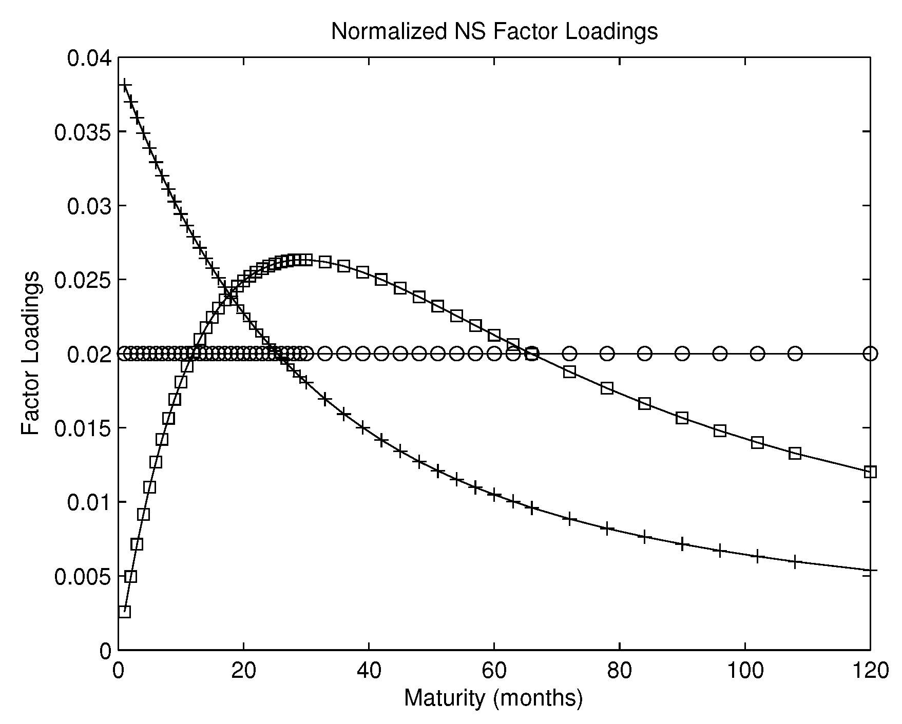
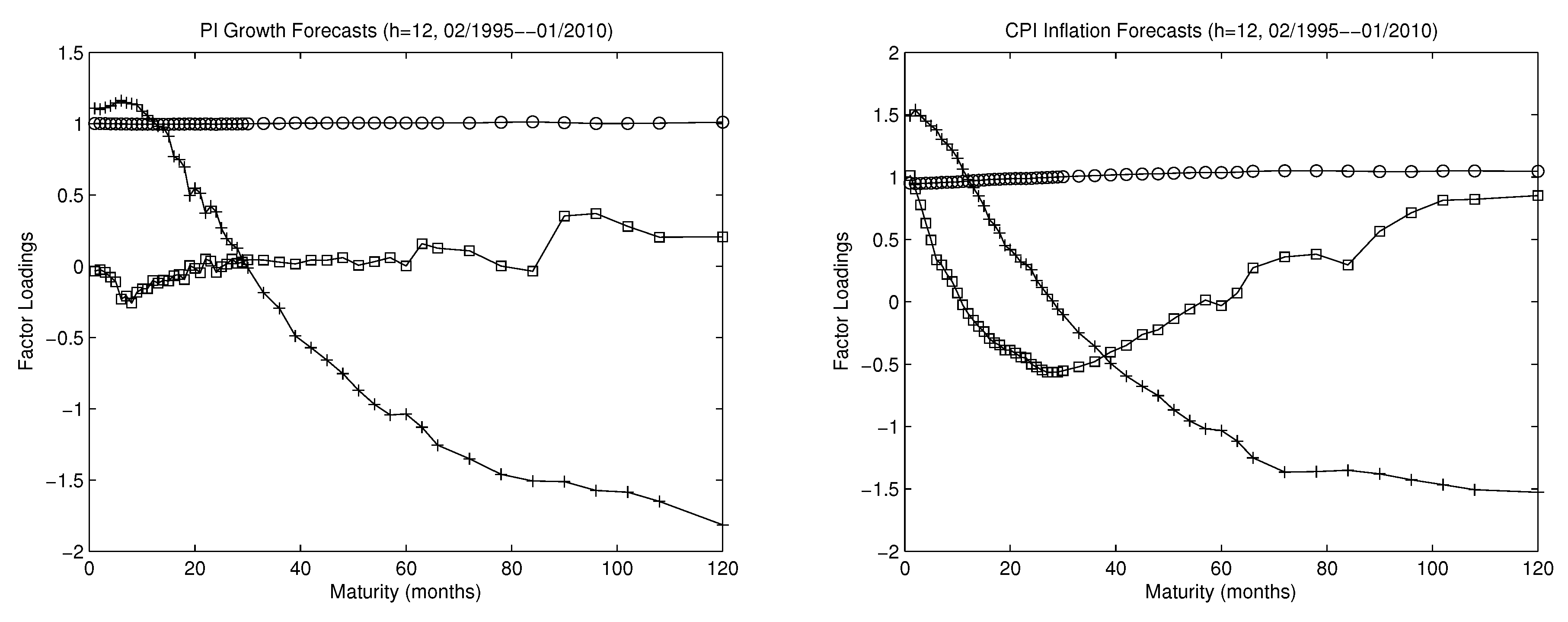
Figure 5 illustrates what economic contents these factors in CF-PC may bear. It shows that the first PC assigns about equal weights to all individual forecasts that use yields at various maturities (in months) so that it may be interpreted as the factor that captures the level of the yield curve; the second PC assigns roughly increasing weights so that it may be interpreted as the factor capturing the slope; and the third PC assigns roughly first decreasing then increasing weights, so that it may be interpreted as factor capturing curvature.
Table 1 and Table 2 present the root mean squared forecast errors (RMSFE) of PC methods with and of NS methods with for PI growth (Table 1A) and for CPI inflation (Table 2A) forecasts using all 50 yield levels.15 In Panel A of Table 1 and Table 2, we report the Root Mean Squared Forecast Errors (RMSFE, which is the squared root of the MSFE of a model).16 In Panel B of Table 1 and Table 2, we report Relative Supervision of CI-PC vs. CF-PC and Relative Supervision of CI-NS vs. CF-NS, according to Definition 3, which is the ratio of the MSFEs of two CI and CF models. The relative supervision in Panel B can be obtained from RMSFEs in Panel A. For simplicity of presentation in Panel B, we present the relative supervision only with the same number of factors ( and .
We find that, in general, supervised factorization performs better. The CF schemes (CF-PC and CF-NS) perform substantially better than the CI schemes (CI-PC and CI-NS). Within the same CF or CI schemes, two alternative factorizations work similarly: CF-PC and CF-NS are about the same, and CI-PC and CI-NS are about the same. We summarize our findings from Figure 5 and Table 1 and Table 2 as follows.
- Supervision is similar for CF-PC and CF-NS. The factor loadings for CF-NS and for CF-PC are similar as shown in Figure 5. Panel (c) of the figure plots three normalized NS exponential loadings in CF-NS that correspond respectively to the three NS factors. Note that the factor loadings in CF-NS are pre-specified while those in CF-PC are estimated from the N individual forecasts. Nevertheless, their shapes in panel (a) look very similar to those of the CF-PC loadings in panels (a) and (b) (apart from the signs). Accordingly, out-of-sample forecasting performance of CF-PC and CF-NS are very similar as shown in Panel A of Table 1 and Table 2.
- We often get the best supervised predictions with a single factor () with the CF-factor models.18 Since CF-NS is the equally weighted combined forecast as noted in Section 4.2.2, this is another case of the forecast combination puzzle discussed in Remark 3 that the equal-weighted forecast combination is hard to beat. Since CF-PC is numerically identical to CF-NS as shown in Figure 5, CF-PC is also effectively equally weighted forecast averaging.19
6. Conclusions
For forecasting in the presence of many predictors, it is often useful to reduce the dimension by a factor model (in a dense case) or by variable selection (in a sparse case). In this paper, we consider a factor model. In particular, we examine the supervised principal component analysis of Chan et al. (1999). The model is called CF-PC, as the principal components of many forecasts are the combined forecasts.
The CF-PC extracts factors from the space spanned by forecasts rather than from the space spanned by predictors. This factorization of the forecasts improves forecast performance compared to factor analysis of the predictors. We extend the CF-PC to CF-NS, which uses the NS factor model in place of the PC factor model, for the application where the predictors are the yield curve. While the yield curve is a functional data consisting of many different maturity points on a curve at each time, the NS factors can parsimoniously capture the shapes of the curve.
We have applied the CF-PC and CF-NS models in forecasting output growth and inflation using a large number of bond yields to examine if the supervised factorization improves forecast performance. In general, we have found that CF-PC and CF-NS perform substantially better than CI-PC and CI-NS, that the advantage of supervised factor models is even larger for longer forecast horizons, and that the two alternative factor models based on PC and NS factors are similar and perform similarly.
Author Contributions
All authors contributed equally to the paper.
Acknowledgments
We would like to thank the two referees for helpful comments. We also thank Jonathan Wright and seminar participants at FRB of San Francisco, FRB of St Louis, Federal Reserve Board (Washington DC), Bank of Korea, SETA meeting, Stanford Institute of Theoretical Economics (SITE), University of Cambridge, NCSU, UC Davis, UCR, UCSB, UCSD, USC, Purdue, LSU, Indiana, Drexel, OCC, WMU, and SNU, for useful discussions and comments. All errors are our own. E.H. acknowledges support from the Danish National Research Foundation. The views presented in this paper are solely those of the authors and do not necessarily represent those of ICBCCS, the Federal Reserve Board or their staff.
Conflicts of Interest
The authors declare no conflict of interest.
Appendix A. Calculation of Absolute and Relative Supervision in Example 1
Using R and obtained from the SVD for CI in (36), and S and obtained from the SVD for CF in (40), we calculate the absolute supervision and relative supervision for each k. The CI factors are from (23), and the CF factors from (28).
For ,
Hence, and
For ,
Hence, and
For ,
Hence, and
For ,
Hence, and
For , because
Hence, as noted in Remark 4, and is not defined for
References
- Ang, Andrew, and Monika Piazzesi. 2003. A No-Arbitrage Vector Autoregression of Term Structure Dynamics with Macroeconomic and Latent Variables. Journal of Monetary Economics 50: 745–87. [Google Scholar] [CrossRef]
- Ang, Andrew, Monika Piazzesi, and Min Wei. 2006. What Does the Yield Curve Tell Us about GDP Growth? Journal of Econometrics 131: 359–403. [Google Scholar] [CrossRef]
- Armah, Nii Ayi, and Norman R. Swanson. 2010. Seeing Inside the Black Box: Using Diffusion Index Methodology to Construct Factor Proxies in Large Scale Macroeconomic Time Series Environments. Econometric Reviews 29: 476–510. [Google Scholar] [CrossRef] [Green Version]
- Bai, Jushan. 2003. Inferential Theory for Factor Models of Large Dimensions. Econometrica 71: 135–71. [Google Scholar] [CrossRef]
- Bai, Jushan, and Serena Ng. 2006. Confidence Intervals for Diffusion Index Forecasts and Inference for Factor-Augmented Regressions. Econometrica 74: 1133–50. [Google Scholar] [CrossRef]
- Bai, Jushan, and Serena Ng. 2008. Forecasting Economic Time Series Using Targeted Predictors. Journal of Econometrics 146: 304–17. [Google Scholar] [CrossRef]
- Bair, Eric, Trevor Hastie, Debashis Paul, and Robert Tibshirani. 2006. Prediction by Supervised Principal Components. Journal of the American Statistical Association 101: 119–37. [Google Scholar] [CrossRef]
- Barndorff-Nielsen, Ole. 1978. Information and Exponential Families in Statistical Theory. New York: Wiley. [Google Scholar]
- Bernanke, Ben. 1990. On the Predictive Power of Interest Rates and Interest Rate Spreads, Federal Reserve Bank of Boston. New England Economic Review November/December: 51–68. [Google Scholar]
- Chan, Lewis, James Stock, and Mark Watson. 1999. A Dynamic Factor Model Framework for Forecast Combination. Spanish Economic Review 1: 91–121. [Google Scholar] [CrossRef]
- Christensen, Jens, Francis Diebold, and Glenn Rudebusch. 2009. An Arbitrage-free Generalized Nelson–Siegel Term Structure Model. Econometrics Journal 12: C33–C64. [Google Scholar] [CrossRef]
- De Jong, Sijmen. 1993. SIMPLS: An Alternative Approach to Partial Least Squares Regression. Chemometrics and Intelligent Laboratory Systems 18: 251–61. [Google Scholar] [CrossRef]
- De Jong, Sijmen, and Henk Kiers. 1992. Principal Covariate Regression: Part I. Theory. Chemometrics and Intelligent Laboratory Systems 14: 155–64. [Google Scholar] [CrossRef]
- Diebold, Francis, and Canlin Li. 2006. Forecasting the Term Structure of Government Bond Yields. Journal of Econometrics 130: 337–64. [Google Scholar] [CrossRef]
- Diebold, Francis, Monika Piazzesi, and Glenn Rudebusch. 2005. Modeling Bond Yields in Finance and Macroeconomics. American Economic Review 95: 415–20. [Google Scholar] [CrossRef]
- Diebold, Francis, Glenn Rudebusch, and Boragan Aruoba. 2006. The Macroeconomy and the Yield Curve: A Dynamic Latent Factor Approach. Journal of Econometrics 131: 309–38. [Google Scholar] [CrossRef]
- Engle, Robert, David Hendry, and Jean-Francois Richard. 1983. Exogeneity. Econometrica 51: 277–304. [Google Scholar] [CrossRef]
- Estrella, Arturo. 2005. Why Does the Yield Curve Predict Output and Inflation? The Economic Journal 115: 722–44. [Google Scholar] [CrossRef]
- Estrella, Arturo, and Gikas Hardouvelis. 1991. The Term Structure as a Predictor of Real Economic Activity. Journal of Finance 46: 555–76. [Google Scholar] [CrossRef]
- Fama, Eugene, and Robert Bliss. 1987. The Information in Long-maturity Forward Rates. American Economic Review 77: 680–92. [Google Scholar]
- Figlewski, Stephen, and Thomas Urich. 1983. Optimal Aggregation of Money Supply Forecasts: Accuracy, Profitability and Market Efficiency. Journal of Finance 38: 695–710. [Google Scholar] [CrossRef]
- Friedman, Benjamin, and Kenneth Kuttner. 1993. Why Does the Paper-Bill Spread Predict Real Economic Activity? In New Research on Business Cycles, Indicators and Forecasting. Edited by James Stock and Mark Watson. Chicago: University of Chicago Press, pp. 213–54. [Google Scholar]
- Gogas, Periklis, Theophilos Papadimitriou, and Efthymia Chrysanthidou. 2015. Yield Curve Point Triplets in Recession Forecasting. International Finance 18: 207–26. [Google Scholar] [CrossRef]
- Groen, Jan, and George Kapetanios. 2016. Revisiting Useful Approaches to Data-Rich Macroeconomic Forecasting. Computational Statistics & Data Analysis 100: 221–39. [Google Scholar]
- Hamilton, James, and Dong Heon Kim. 2002. A Reexamination of the Predictability of Economic Activity Using the Yield Spread. Journal of Money, Credit, and Banking 34: 340–60. [Google Scholar] [CrossRef]
- Huang, Huiyu, and Tae-Hwy Lee. 2010. To Combine Forecasts or To Combine Information? Econometric Reviews 29: 534–70. [Google Scholar] [CrossRef]
- Inoue, Atsushi, and Lutz Kilian. 2008. How Useful is Bagging in Forecasting Economic Time Series? A Case Study of U.S. CPI Inflation. Journal of the American Statistical Association 103: 511–22. [Google Scholar] [CrossRef]
- Kozicki, Sharon. 1997. Predicting Real Growth and Inflation with the Yield Spread, Federal Reserve Bank of Kansas City. Economic Review 82: 39–57. [Google Scholar]
- Lancaster, Tony. 2000. The incidental parameter problem since 1948. Journal of Econometrics 95: 391–413. [Google Scholar] [CrossRef] [Green Version]
- Litterman, Robert, and Jose Scheinkman. 1991. Common Factors Affecting Bond Returns. Journal of Fixed Income 1: 54–61. [Google Scholar] [CrossRef]
- Nelson, Charles, and Andrew Siegel. 1987. Parsimonious Modeling of Yield Curves. Journal of Business 60: 473–89. [Google Scholar] [CrossRef]
- Neyman, Jerzy, and Elizabeth Scott. 1948. Consistent Estimation from Partially Consistent Observations. Econometrica 16: 1–32. [Google Scholar] [CrossRef]
- Piazzesi, Monika. 2005. Bond Yields and the Federal Reserve. Journal of Political Economy 113: 311–44. [Google Scholar] [CrossRef]
- Rudebusch, Glenn, and Tao Wu. 2008. A Macro-Finance Model of the Term Structure, Monetary Policy, and the Economy. Economic Journal 118: 906–26. [Google Scholar] [CrossRef]
- Smith, Jeremy, and Kenneth Wallis. 2009. A Simple Explanation of the Forecast Combination Puzzle. Oxford Bulletin of Economics and Statistics 71: 331–55. [Google Scholar] [CrossRef]
- Stock, James, and Mark Watson. 1989. New Indexes of Coincident and Leading Indicators. In NBER Macroeconomic Annual. Edited by Olivier Blanchard and Stanley Fischer. Cambridge: MIT Press, vol. 4. [Google Scholar]
- Stock, James, and Mark Watson. 1999. Forecasting Inflation. Journal of Monetary Economics 44: 293–335. [Google Scholar] [CrossRef]
- Stock, James, and Mark Watson. 2002. Forecasting Using Principal Components from a Large Number of Predictors. Journal of the American Statistical Association 97: 1167–79. [Google Scholar] [CrossRef]
- Stock, James, and Mark Watson. 2004. Combination Forecasts of Output Growth in a Seven-country Data Set. Journal of Forecasting 23: 405–30. [Google Scholar] [CrossRef]
- Stock, James, and Mark Watson. 2007. Has Inflation Become Harder to Forecast? Journal of Money, Credit, and Banking 39: 3–34. [Google Scholar] [CrossRef]
- Stock, James, and Mark Watson. 2012. Generalized Shrinkage Methods for Forecasting Using Many Predictors. Journal of Business and Economic Statistics 30: 481–93. [Google Scholar] [CrossRef]
- Svensson, Lars. 1995. Estimating Forward Interest Rates with the Extended Nelson–Siegel Method. Quarterly Review 3: 13–26. [Google Scholar]
- Tibshirani, Robert. 1996. Regression Shrinkage and Selection via the Lasso. Journal of the Royal Statistical Society B 58: 267–88. [Google Scholar]
- Timmermann, Alan. 2006. Forecast Combinations. In Handbook of Economic Forecasting. Edited by Graham Elliott, Clive Granger and Alan Timmermann. Amsterdam: North-Holland, vol. 1, chp. 4. [Google Scholar]
- Wright, Jonathan. 2009. Forecasting US Inflation by Bayesian Model Averaging. Journal of Forecasting 28: 131–44. [Google Scholar] [CrossRef]
- Zou, Hui, Trevor Hastie, and Robert Tibshirani. 2006. Sparse Principal Component Analysis. Journal of Computational and Graphical Statistics 15: 262–86. [Google Scholar] [CrossRef]
| 1 | |
| 2 | Bai and Ng (2008) consider CI factor models with a selected subset (targeted predictors). |
| 3 | The suppressed time stamp of y and X captures the h-lag relation for the forecast horizon and we treat the data centered so that we do not include a constant term explicitly in the regression for notational simplicity. |
| 4 | Given the dependent nature of macroeconomic and financial time series, the forecasting equation can be extended to allow the supervision to be based on the relation between yt and some predictors after controlling for lagged dependent variables and to allow the dynamic factor structure, which we leave for future work. |
| 5 | |
| 6 | |
| 7 | In relation to the empirical application using the yield data in Section 5, we could have calibrated the simulation design to make the Monte Carlo more realistic for the empirical application in Section 5. Nevertheless, our Monte Carlo design covers wide ranges of the parameter values for the noise levels, correlation structures ( and ) in the yield data. Figure 2 shows that the supervision is smaller with larger noise levels, which may be rather obvious intuitively. Figure 4 shows that the advantage of supervision when the factors are persistence, which depends on the number of factors k relative to the true number of factors r. Particularly interesting is Figure 3 which shows that the advantage of supervision is smaller when the contemporaneous correlation between predictors is larger, which may be relevant for the yield data because the yields with different maturities may be moderately contemporaneously correlated. We thank a referee for pointing this out. |
| 8 | Diebold and Li (2006) show that fixing Nelson–Siegel decay parameter at maximizes the curvature loading at the two-year bond maturity and allows better identifications of the three NS factors. They also show that allowing the to be a free parameter does not improve the forecasting performance. Therefore, following their advice, we fix and did not estimate it. A small (for a slow decaying curve) fits the curve for long maturities better and a large (for a fast decaying curve) fits the curve for short maturities better. |
| 9 | is used in Bai and Ng (2008). |
| 10 | As a robust check, we apply our method to the original yield data of Diebold and Li (2006) and also to the sub-samples in our data set. The results are essentially the same as those summarized at the end of Section 5. |
| 11 | It may be interesting to explore whether different maturity yields might have different effects on the forecast outcome. However, the present paper is focused on the comparison between CF and CI, rather than a detailed CI-only analysis, e.g., to find the best maturity yield for the forecast outcome. Nevertheless, our CI-NS model has reflected such effects as the three NS factors (level, slope, and curvature) are different combinations of bond maturities as shown in Equation (55). The different coefficients on the NS factors suggest that different bond maturities have different effects on the forecast outcome, as Gogas et al. (2015) has found. |
| 12 | While not reported for space, we tried forecasting change in inflation and found forecasting inflation directly using all yield levels improves out-of-sample performances of most forecasting methods by a large margin. |
| 13 | As a robust check, we have also tried with different sample splits for the estimation and prediction periods, i.e., the number of in-sample regression observations and the out-of-sample evaluation observations. We find that the results are similar. |
| 14 | For different values of , the performances of CI-NS and CF-NS change only marginally. |
| 15 | While we report the results for for CF-PC, we do not report for for CF-NS. Svennsson (1995) and Christensen et al. (2009) (CDR 2009) extend the three factor NS model to four or five factor NS models. CDR’s dynamic generalized NS model has five factors with one level factor, two slope factors and two curvature factors. The Svensson and CDR extensions are useful to fit the yield curve at longer maturities (>10 years). Because we only used yields with maturities ≤10 years, the second curvature factor loadings will look similar to the slope factor loadings and we will have collinearity problem. CDR use yields up to 30 years. The 4th and 5th factors have no clear economic intrepretations and are hard to explain. For these reasons, we report results for for the CF-NS model. |
| 16 | For the statistical significance of the loss-difference (see Definition 2), the asymptotic p-values of the Diebold–Mariano statistics are all very close to zero especially for larger values of the forecast horizon |
| 17 | We conducted a Monte Carlo (not reported), which are consistent with the empirical results that the supervision is stronger for a longer forecast horizon |
| 18 | Figlewski and Urich (1983) talked about various constrained models in forming a combination of forecasts and examined when we need more than the simple averaging combined forecast. They discussed a sufficient condition when the simple average of forecasts is the optimal forecast combination: “Under the most extensive set of constraints, forecast errors are assumed to have zero mean and to be independent and identically distributed. In this case the optimal forecast is the simple average.” This corresponds to CF-PC() and CF-NS when the first factor in PC or NS is sufficient for the CF factor model. It is clearly the case in CF-NS as shown in Equation (55). One can show that the first PC (corresponding to the largest singular value) would also be the simple average. Hence, in terms of the CF-factor model, the forecast combination puzzle amounts to the fact that we often do not need the second PC factor. Interestingly, (Figlewski and Urich 1983, p. 696) continued to note the cases when the simple average is not optimal: “However, the hypothesis of independence among forecast errors is overwhelmingly rejected for our data-errors are highly positively correlated with one another.” On the other hand, they also noted other reasons why the simple average may still be preferred, as they wrote, “Because the estimated error structure was not completely stable over time, the models which adjusted for correlation did not achieve lower mean squared forecast error than the simple average in out-of-sample tests. Even so, we find...that forecasts from these models, while less accurate than the simple mean, do contain information which is not fully reflected in prices in the money market, and is therefore economically valuable.” We thank a referee for letting us know on this from Figlewski and Urich (1983). |
| 19 | While the simple equally weighted forecast combination can be implemented without the use of PCA or without making reference to the NS model, it is important to note that the simple average combined forecast indeed corresponds the first CF-PC factor (CF-PC) or the first CF-NS factor (CF-NS). In view of Figlewski and Urich (1983), it will be useful to know when the first factor is enough so that the simple average is good or when the higher order factors may be necessary as they contain more information in addition to the first CF-factor. This is important in understanding the forecast combination puzzle. The forecast combination puzzle is about whether to include only the first CF factor or more. |
Figure 1.
For Example 2. Monte Carlo averages of the sum of squared errors (SSE) against a grid of standard deviations ranging from 0.01 to 3 in factor and forecast equations, for a selection of to components. When the standard deviation is close to zero, the SSE are close to the ones reported in Example 1. With increasing noise, the advantage of CF over CI decreases but remains substantial, in particular for few components. For (not shown), the SSE of CI-PC and CF-PC coincide, as shown in Remark 4.
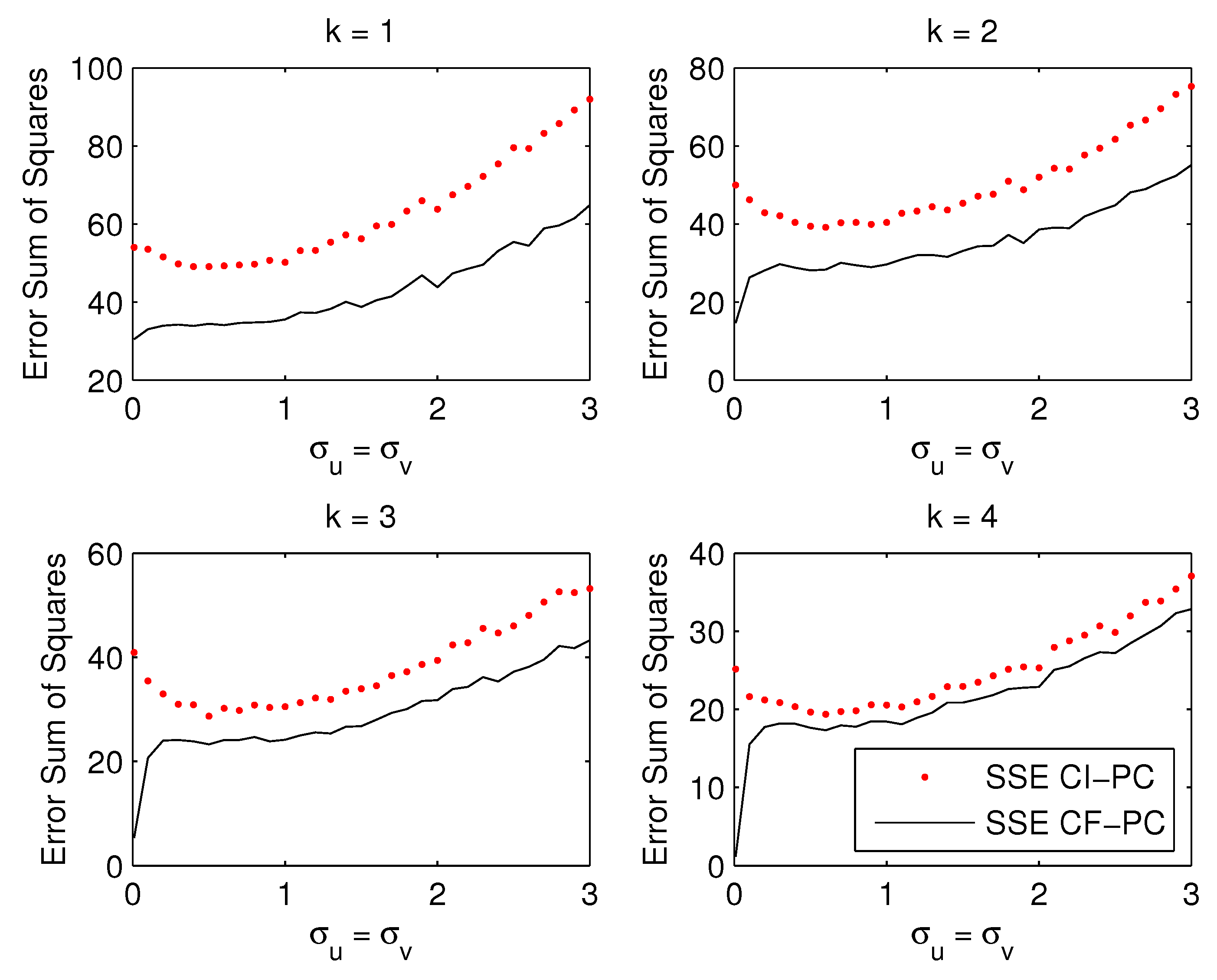
Figure 2.
Supervision dependent on noise. Relative supervision against a grid of standard deviations in factor and forecast equation , ranging from 0.01 to 3, while the factor serial correlation is fixed at and the contemporaneous factor correlation is .
Figure 2.
Supervision dependent on noise. Relative supervision against a grid of standard deviations in factor and forecast equation , ranging from 0.01 to 3, while the factor serial correlation is fixed at and the contemporaneous factor correlation is .

Figure 3.
Supervision dependent on contemporaneous factor correlation Relative supervision against a grid of contemporaneous correlation coefficients ranging from to while the factor serial correlation is fixed at zero and the noise level is fixed at .
Figure 3.
Supervision dependent on contemporaneous factor correlation Relative supervision against a grid of contemporaneous correlation coefficients ranging from to while the factor serial correlation is fixed at zero and the noise level is fixed at .

Figure 4.
Supervision dependent on factor persistence Relative supervision against a grid of AR(1) coefficients ranging from 0 to 0.9, while the noise level is fixed at and the contemporaneous regressor correlation is .
Figure 4.
Supervision dependent on factor persistence Relative supervision against a grid of AR(1) coefficients ranging from 0 to 0.9, while the noise level is fixed at and the contemporaneous regressor correlation is .

Figure 5.
Factor loadings of principal components and Nelson–Siegel factors. The first two panels: factor loadings of the first three principal components in CF-PC () averaged over the out-of-sample period (02/1995–01/2010), for both PI growth (first panel) and CPI inflation (second panel). The abscissa refers to the 50 individual forecasts that use yields at the 50 maturities (in months). The loading of the first principal component has the circle-symbol, the second the cross-symbol, and the third the square-symbol. The third panel: three normalized Nelson–Siegel (NS) exponential loadings in CF-NS that correspond to the three NS factors, respectively. The abscissa refers to the 50 individual forecasts that use yields at the 50 maturities (in months). The circled line denotes the first normalized NS factor loading , the crossed line denotes the second normalized NS factor loading , divided by the sum, and the squared line denotes the third normalized NS factor loading , divided by the sum, where denotes maturity and is fixed at 0.0609.


Table 1.
Out-of-sample forecasting of personal income growth.
| Panel A. Root Mean Squared Forecast Errors | ||||||||
| CI-PC() | 5.64 | 3.56 | 2.99 | 2.78 | 2.61 | 2.50 | 2.46 | 2.42 |
| CI-PC() | 5.67 | 3.64 | 3.12 | 3.00 | 2.81 | 2.66 | 2.55 | 2.45 |
| CI-PC() | 5.71 | 3.69 | 3.19 | 3.08 | 2.92 | 2.77 | 2.63 | 2.49 |
| CI-PC() | 5.72 | 3.76 | 3.23 | 3.12 | 2.93 | 2.77 | 2.58 | 2.36 |
| CI-PC() | 5.74 | 3.78 | 3.26 | 3.15 | 2.98 | 2.81 | 2.61 | 2.38 |
| CI-NS() | 5.84 | 3.84 | 3.28 | 3.06 | 2.86 | 2.69 | 2.53 | 2.41 |
| CI-NS() | 5.71 | 3.71 | 3.20 | 3.11 | 2.93 | 2.77 | 2.62 | 2.48 |
| CI-NS() | 5.72 | 3.69 | 3.19 | 3.09 | 2.93 | 2.78 | 2.63 | 2.47 |
| CF-PC() | 5.60 | 3.45 | 2.83 | 2.54 | 2.24 | 1.95 | 1.75 | 1.58 |
| CF-PC() | 5.56 | 3.43 | 2.83 | 2.62 | 2.31 | 1.93 | 1.76 | 1.61 |
| CF-PC() | 5.60 | 3.44 | 2.94 | 2.78 | 2.47 | 2.02 | 1.65 | 1.48 |
| CF-PC() | 5.63 | 3.60 | 3.08 | 2.83 | 2.39 | 1.97 | 1.67 | 1.45 |
| CF-PC() | 5.63 | 3.60 | 3.05 | 2.87 | 2.41 | 2.05 | 1.69 | 1.51 |
| CF-NS() | 5.60 | 3.45 | 2.83 | 2.54 | 2.24 | 1.95 | 1.75 | 1.58 |
| CF-NS() | 5.56 | 3.43 | 2.84 | 2.62 | 2.30 | 1.95 | 1.76 | 1.62 |
| CF-NS() | 5.59 | 3.44 | 2.94 | 2.79 | 2.47 | 2.02 | 1.64 | 1.48 |
| Panel B. Relative Supervision | ||||||||
| CI-PC() vs. CF-PC() | 1.01 | 1.06 | 1.12 | 1.20 | 1.36 | 1.64 | 1.98 | 2.35 |
| CI-PC() vs. CF-PC() | 1.04 | 1.13 | 1.22 | 1.31 | 1.48 | 1.90 | 2.10 | 2.32 |
| CI-PC() vs. CF-PC() | 1.04 | 1.15 | 1.18 | 1.23 | 1.40 | 1.88 | 2.54 | 2.83 |
| CI-PC() vs. CF-PC() | 1.03 | 1.09 | 1.10 | 1.22 | 1.50 | 1.98 | 2.39 | 2.65 |
| CI-PC() vs. CF-PC() | 1.04 | 1.10 | 1.14 | 1.20 | 1.53 | 1.88 | 2.39 | 2.48 |
| CI-NS() vs. CF-NS() | 1.09 | 1.24 | 1.34 | 1.45 | 1.63 | 1.90 | 2.09 | 2.33 |
| CI-NS() vs. CF-NS() | 1.05 | 1.17 | 1.27 | 1.41 | 1.62 | 2.02 | 2.22 | 2.34 |
| CI-NS() vs. CF-NS() | 1.05 | 1.15 | 1.18 | 1.23 | 1.41 | 1.89 | 2.57 | 2.79 |
The forecast target is Output Growth Out-of-sample forecasting period is 02/1995–01/2010. In Panel A, reported are the Root Mean Squared Forecast Errors (which is the squared root of the MSFE of a model). In Panel B, reported are Relative Supervision of CI-PC vs. CF-PC and Relative Supervision of CI-NS vs. CF-NS, according to Definition 3, which is the ratio of the MSFEs of the two models. For simplicity of presentation, we present the relative supervision in Panel B only with the same number of factors ( and .
Table 2.
Out-of-sample forecasting of CPI inflation.
| Panel A. Root Mean Squared Forecast Errors | ||||||||
| CI-PC() | 3.77 | 2.86 | 2.25 | 1.92 | 1.94 | 2.16 | 2.47 | 2.75 |
| CI-PC() | 4.21 | 3.45 | 2.96 | 2.76 | 2.77 | 2.84 | 2.96 | 3.08 |
| CI-PC() | 4.24 | 3.50 | 3.00 | 2.82 | 2.88 | 2.98 | 3.10 | 3.19 |
| CI-PC() | 4.31 | 3.57 | 3.05 | 2.87 | 2.91 | 3.00 | 3.12 | 3.18 |
| CI-PC() | 4.30 | 3.58 | 3.07 | 2.93 | 3.00 | 3.10 | 3.20 | 3.23 |
| CI-NS() | 3.95 | 3.12 | 2.62 | 2.48 | 2.60 | 2.79 | 2.97 | 3.10 |
| CI-NS() | 4.22 | 3.46 | 2.98 | 2.82 | 2.88 | 2.98 | 3.09 | 3.18 |
| CI-NS() | 4.24 | 3.50 | 3.01 | 2.83 | 2.89 | 2.99 | 3.11 | 3.20 |
| CF-PC() | 3.65 | 2.67 | 1.91 | 1.31 | 1.01 | 0.90 | 0.96 | 1.08 |
| CF-PC() | 3.66 | 2.70 | 1.93 | 1.35 | 1.10 | 1.05 | 1.11 | 1.19 |
| CF-PC() | 3.68 | 2.72 | 1.97 | 1.47 | 1.29 | 1.19 | 1.19 | 1.20 |
| CF-PC() | 3.74 | 2.80 | 2.01 | 1.47 | 1.22 | 1.14 | 1.15 | 1.17 |
| CF-PC() | 3.74 | 2.79 | 1.98 | 1.45 | 1.20 | 1.12 | 1.18 | 1.20 |
| CF-NS() | 3.65 | 2.68 | 1.91 | 1.31 | 1.02 | 0.90 | 0.96 | 1.08 |
| CF-NS() | 3.66 | 2.70 | 1.93 | 1.35 | 1.10 | 1.05 | 1.10 | 1.19 |
| CF-NS() | 3.68 | 2.73 | 1.97 | 1.47 | 1.29 | 1.20 | 1.19 | 1.20 |
| Panel B. Relative Supervision | ||||||||
| CI-PC() vs. CF-PC() | 1.07 | 1.15 | 1.39 | 2.15 | 3.69 | 5.76 | 6.62 | 6.48 |
| CI-PC() vs. CF-PC() | 1.32 | 1.63 | 2.35 | 4.18 | 6.34 | 7.32 | 7.11 | 6.70 |
| CI-PC() vs. CF-PC() | 1.33 | 1.66 | 2.32 | 3.68 | 4.98 | 6.27 | 6.79 | 7.07 |
| CI-PC() vs. CF-PC() | 1.33 | 1.63 | 2.30 | 3.81 | 5.69 | 6.93 | 7.36 | 7.39 |
| CI-PC() vs. CF-PC() | 1.32 | 1.65 | 2.40 | 4.08 | 6.25 | 7.66 | 7.35 | 7.25 |
| CI-NS() vs. CF-NS() | 1.17 | 1.36 | 1.88 | 3.58 | 6.50 | 9.61 | 9.57 | 8.24 |
| CI-NS() vs. CF-NS() | 1.33 | 1.64 | 2.38 | 4.36 | 6.85 | 8.05 | 7.89 | 7.14 |
| CI-NS() vs. CF-NS() | 1.33 | 1.64 | 2.33 | 3.71 | 5.02 | 6.21 | 6.83 | 7.11 |
The forecast target is Inflation Out-of-sample forecasting period is 02/1995–01/2010. In Panel A, reported are the Root Mean Squared Forecast Errors (which is the squared root of the MSFE of a model). In Panel B, reported are Relative Supervision of CI-PC vs. CF-PC and Relative Supervision of CI-NS vs. CF-NS, according to Definition 3, which is the ratio of the MSFEs of the two models. For simplicity of presentation, we present the relative supervision in Panel B only with the same number of factors ( and .
© 2018 by the authors. Licensee MDPI, Basel, Switzerland. This article is an open access article distributed under the terms and conditions of the Creative Commons Attribution (CC BY) license (http://creativecommons.org/licenses/by/4.0/).
Share and Cite
MDPI and ACS Style
Hillebrand, E.; Huang, H.; Lee, T.-H.; Li, C. Using the Entire Yield Curve in Forecasting Output and Inflation. Econometrics 2018, 6, 40. https://doi.org/10.3390/econometrics6030040
AMA Style
Hillebrand E, Huang H, Lee T-H, Li C. Using the Entire Yield Curve in Forecasting Output and Inflation. Econometrics. 2018; 6(3):40. https://doi.org/10.3390/econometrics6030040
Chicago/Turabian StyleHillebrand, Eric, Huiyu Huang, Tae-Hwy Lee, and Canlin Li. 2018. "Using the Entire Yield Curve in Forecasting Output and Inflation" Econometrics 6, no. 3: 40. https://doi.org/10.3390/econometrics6030040
Note that from the first issue of 2016, this journal uses article numbers instead of page numbers. See further details here.