
A Spatial Econometric Analysis of the Calls to the Portuguese National Health Line †
by
 , ,
, ,
Paula Simões
1,2,* ,
,
M. Lucília Carvalho
3,4,
Sandra Aleixo
2,3,
Sérgio Gomes
5 and
Isabel Natário
1,6 1
Centro de Matemática e Aplicações (CMA), Universidade Nova de Lisboa, 2829-516 Caparica, Portugal
2
Área Departamental de Matemática, ISEL—Instituto Superior de Engenharia de Lisboa, Instituto Politécnico de Lisboa, 1959-007 Lisboa, Portugal
3
Centro de Estatística e Aplicações (CEAUL), Universidade de Lisboa, 1749-016 Lisboa, Portugal
4
Faculdade de Ciências, Universidade de Lisboa, 1749-016 Lisboa, Portugal
5
Direção Geral de Saúde (DGS), 1049-005 Lisboa, Portugal
6
Departamento de Matemática, Faculdade de Ciências e Tecnologia, Universidade Nova de Lisboa, 2829-516 Caparica, Portugal
*
Author to whom correspondence should be addressed.
†
This paper is an extended version of our paper published in Simões, P.; Natário, I.; Aleixo, S.; Gomes, S., A Spatial econometric analysis of the calls to a national health line to assess hospital savings, Proceedings X World Conference of Spatial Econometrics Association-SEA2016 –Università Cattolica del Sacro Cuore, Rome, 13–15 June 2016.
Econometrics 2017, 5(2), 24; https://doi.org/10.3390/econometrics5020024
Submission received: 31 January 2017
/
Revised: 30 May 2017
/
Accepted: 31 May 2017
/
Published: 16 June 2017
(This article belongs to the Special Issue Recent developments in Spatial Econometrics, associated with the 10th Annual Conference of the Spatial Econometrics Association, Rome 13-15 June 2016)
Abstract
:The Portuguese National Health Line, LS24, is an initiative of the Portuguese Health Ministry which seeks to improve accessibility to health care and to rationalize the use of existing resources by directing users to the most appropriate institutions of the national public health services. This study aims to describe and evaluate the use of LS24. Since for LS24 data, the location attribute is an important source of information to describe its use, this study analyses the number of calls received, at a municipal level, under two different spatial econometric approaches. This analysis is important for future development of decision support indicators in a hospital context, based on the economic impact of the use of this health line. Considering the discrete nature of data, the number of calls to LS24 in each municipality is better modelled by a Poisson model, with some possible covariates: demographic, socio-economic information, characteristics of the Portuguese health system and development indicators. In order to explain model spatial variability, the data autocorrelation can be explained in a Bayesian setting through different hierarchical log-Poisson regression models. A different approach uses an autoregressive methodology, also for count data. A log-Poisson model with a spatial lag autocorrelation component is further considered, better framed under a Bayesian paradigm. With this empirical study we find strong evidence for a spatial structure in the data and obtain similar conclusions with both perspectives of the analysis. This supports the view that the addition of a spatial structure to the model improves estimation, even in the case where some relevant covariates have been included.
JEL Classification:
C49; C111. Introduction
An initiative to improve accessibility to health care and to rationalize the use of existing resources was carried out by the Portuguese Health Ministry through the creation of a national health line, LS24, in April 2007 (Portal of the National Portuguese Health Service 2015). These objectives are accomplished by the LS24 service which directs users to the most appropriate institutions of the national public health service or by counseling self-care home measures.
This study analyses the number of calls to LS24 at a municipal level, as the location attribute for LS24 data is an important source of information to describe its use, with a view to a future development of decision support indicators in a hospital context based on the economic impact of the use of LS24 rather than on the criterion of hospital urgency. As space is an important feature of these data, ignoring it results in a poorer analysis (Anselin et al. 1996; Cressie 1993).
To model the number of calls to LS24 in each municipality with spatial models, given the discrete nature of data (counts), an alternative is to use a hierarchical Bayesian model with covariates (Banerjee et al. 2004). This approach allows data to have any distribution where, in this case, the Poisson is the obvious choice. The spatial structure assumed for the risk of what is being counted is included, in the first level of the hierarchy, through a prior distribution of spatially structured random effects. In addition, some non-spatially structured random effects to account for risk variation not as yet explained can be considered. These models are better considered under the Bayesian paradigm and their inference needs to be based on simulation methods, namely the Markov Chain Monte Carlo (MCMC) method (Doucet et al. 2001).
For the hierarchical approach spatial autocorrelation is accounted for in the disturbances and not in the observed responses, as happens with spatial autoregressive approaches. The latter is a different modelling strategy common in spatial econometrics literature that may also be considered for these data. It is plausible to think that the number of calls to LS24 in one municipality is related to the number of calls in the municipalities of its neighbourhood, driven by effects of covariates such as the number of hospitals in one municipality, which may certainly have an impact on the number of calls to LS24 in a neighbouring municipality, or others not considered in the modelling (Lesage and Pace 2009). Hierarchical and autoregressive modelling perspectives have already been used to model the same data sets (Bivand et al. 2014a; Goméz-Rubio et al. 2014; Quddus 2008).
Traditional spatial econometric models, such as the spatial lag autoregressive model (slm) and the spatial error model (sem), rely however on the gaussian assumption of the response variable (Lesage and Pace 2009), which no longer holds true for the number of calls (counts). Consequently their usage for count data, such as the number of calls, demands data transformation to meet the assumptions of the models. Nevertheless in the scope of these spatial autoregressive models there are alternatives for modelling counts that we explore here. A spatial lag autoregressive component is incorporated in the model for counts, under a Bayesian paradigm and using Integrated Nested Laplace Approximations (INLA) methodology (Rue et al. 2009), taking into consideration a standard spatial lag model, as recently developed within a new class of latent models defined in INLA by Goméz-Rubio et al. (2015) and also taking into account a spatial autoregressive lag model of counts developed by Lambert et al. (2010), under a classical perspective. The model is implemented in R-INLA. Combining the two referred models results in a spatial lag Poisson model, a proposed alternative to do Bayesian inference in spatial econometric models for count data.
Both hierarchical and autoregressive approaches are not yet much explored for spatial econometric models for non-Gaussian data, but they are surely more adequate for these, avoiding data transformation and corresponding to more realistic models.
Regarding the study of the number of calls to LS24, firstly standard spatial econometric techniques are used to look for spatial dependence in the number of calls to LS24 in each municipality, considering a neighbourhood contiguity structure, as well as in the residuals of a baseline log-Poisson model with covariates. The number of calls is further analysed, on one hand, through different hierarchical log-Poisson models, and on the other hand, through a spatial lag Poisson model, implementing different econometric approaches to model spatial structure in data. The results of this study are intended to be used in the near future in cooperation with the Portuguese Directorate-General of Health to analyse, test, implement and predict consequences of different government management policies at hospital level under distinct scenarios. The savings from the correct use the LS24 will avoid unnecessary urgent care in hospitals that can then be channeled towards other needy areas.
This work is organised as follows: Section 2 is divided into two parts: (a) elaboration of some exploratory spatial techniques to look for spatial correlation and (b) description of Bayesian hierarchical models and Bayesian autoregressive models, both for Poisson count data. These methodologies are used in the following section for modelling the number of calls to LS24 in each municipality in 2014. Section 4 discusses the main results as well as some perspectives for future work.
2. Materials and Methods
Count data are typically modelled through Poisson regression models, classically not considering space dimension. However, when justified, the inclusion of a spatial component in these models is possible in a hierarchically or autoregressive way, both under a Bayesian paradigm, considering count data in areas or spatial units known as “Lattice Data” (Banerjee et al. 2004; Besag 1974; Cressie 1993).
2.1. Spatial Dependence
Spatial association, also referred to as spatial autocorrelation, is present in situations where observations or spatial units are non-independent over space, that is, when nearby spatial units are associated in some way (Cressie 1993). Such association can be identified in a number of ways, for example, using a scatter-plot where each value is plotted against the mean of neighbouring areas—the Moran’s scatter plot, or using a spatial autocorrelation statistic such as Moran’s I or Geary’s C. Moran’s I is a measure of global spatial autocorrelation, while Geary’s C is more sensitive to local spatial autocorrelation (Carvalho and Natário 2008).
Both these statistics require the choice of a spatial weights matrix, usually symmetric and denoted by the letter W (with elements , where n is the number of spatial units), that represents the topology or spatial arrangement of the data and our understanding of spatial association among all areas units (Fischer 2006). Usually, , but for , the association measure between area i and area j, , can be defined in many different ways, the most usual and the one used in this work being the contiguity criterion between areas for which only if areas i and j share a common border and elsewhere (Carvalho and Natário 2008).
Moran’s I Statistics
The Moran’s I statistics is one of the most used statistics to measure spatial association. This statistics can be applied directly to the dependent variable or to the residuals of a fitted model, and it is formally given by
representing y the quantity of interest.
For I statistics, tests for the null hypotheses of spatial independence can be built under two different situations: a randomized statistics distribution or a normal approximation. A significantly positive value of I indicates the presence of direct spatial correlation, a significantly negative value an inverse spatial correlation and when I is close to zero the absence of spatial correlation. Note that for relatively small values of n, the I distribution can be far away from the normal distribution and the randomized test is preferred.
When spatial autocorrelation is identified, due to its distinct nature, a specialized set of statistical methods is needed (Arbia 2006; Lesage 1999). In order to capture dependencies across spatial units, spatially correlated variables can be introduced in the model specification (Anselin 2010).
2.2. Spatial Models for Count Data—Hierarchical Bayesian Approach
In order to use traditional econometric models for continuous data to model count data, defined into spatial units of a lattice, it is necessary to transform the discrete dependent variable to meet the required assumptions (Lesage 1999). However, there are some alternative models which can be applied directly to count data, wherein the spatial dependency structure is defined conditionally.
Part of the spatial autocorrelation can be accommodated by including known covariate risk factors in a generalized linear regression model, but it is common that spatial structure remains in the residuals after accounting for these covariate effects. For modelling the residual autocorrelation, the most common approach is to expand the linear predictor with a set of spatially correlated random effects, as a part of a Bayesian hierarchical model (Banerjee et al. 2004).
The referred random effects are usually modeled by a conditional autoregressive (CAR) model (Besag et al. 1991), which induces a priori spatial autocorrelation through the contiguity structure of the spatial units. Different CAR prior distributions commonly used for modelling spatial autocorrelation have been establish in the literature: from the Besag, York and Mollié (BYM) proposal (Besag et al. 1991), to the alternatives developed by Leroux et al. (1999) and Stern and Cressie (1999), where each model is a special case of a Gaussian Markov Random Field (GMRF).
The general model is a generalized linear mixed model for spatial areal unit data, where the responses are assumed to be distributed as a member of the exponential family of distributions, such as the Poisson distribution. The next subsection describes and explains different Bayesian hierarchical models for Poisson count data.
2.2.1. Hierarchical log-Poisson regression model
Considering a spatial domain divided into n spatial units (or areas), let and represent, respectively, the number of observed and expected cases of what is being measured in each spatial unit, the latter obtained by some standardization procedure. The counts are assumed to be Poisson distributed with expected value , where is the relative risk in area i. Let denote a set of k covariates measured in spatial unit i, for , the first of which corresponds to the intercept term and let be the corresponding regression coefficients. This notation is assumed for the rest of the paper.
The general hierarchical log-Poisson regression model is defined as:
where , , the log relative risks (Dass et al. 2010; Lee 2014). Note that enter as known offsets in the model.
In (2), the log relative risks are decomposed into the effects of covariates plus some random effects that are able to account for possible over-dispersion:
When spatial autocorrelation is detected in data, the spatial structure can be considered through a global CAR prior, here considered with two different approaches, the Besag-York-Mollié and the Leroux models. The CAR specification defines prior conditional distributions for the spatial random effects , where the distribution of conditioned on the other , where , is given, depending only on the neighbours of each area, according to the chosen spatial structure. CAR prior is then specified as a set of n univariate full conditional distributions, , for , rather than via the multivariate specification (Besag 1974).
Besag-York-Mollié Model
The BYM model by Besag et al. (1991) comprises two sets of random effects, spatially correlated () and unstructured random effects (), that is in (3). The unstructured random effects partially accounts for possible effects of over-dispersion and are implemented with the exchangeable prior,
The variance parameter is assigned an Inverse-Gamma prior on the interval , with large (here taken to be 1000). For the spatial random effects, a CAR prior is proposed, where the conditional expectation of each effect is given as the average of the random effects in neighbouring areas, while the conditional variance is inversely proportional to the number of neighbours.
Leroux, Lei and Breslow Model
The previous model requires two random effects to be estimated for each data point, whereas only their sum is identifiable from data. To get through this, Leroux et al. (1999) proposed an alternative CAR prior for modelling spatial autocorrelation, using a single set of random effects for modelling varying strengths of spatial autocorrelation, that is in (3). The prior distribution of the random effects is given by
where is a spatial autocorrelation parameter, with corresponding to independence and corresponding to strong spatial autocorrelation. An uniform prior on the unit interval is specified for , , and a Inverse-Gamma prior on the interval is adopted for , with large (here taken to be 1000).
The CAR priors defined for these models enforce a single global level of spatial smoothing for the set of random effects, which, for the Leroux model, is controlled by .
The inference for these methods is based on MCMC simulation.
2.3. Spatial Autoregressive Bayesian Models for Count Data
Spatial patterns can be modelled differently through autoregressive models, very common in spatial econometrics literature, in which spatial dependence is included in a way such that the value of one observation is dependent on the value of its neighbour observations (Bivand et al. 2014b). This approach is also valid for count data when it is plausible to think that the space relation between these counts is driven by the effects of covariates whose values in one area may impact the counts in that area neighbourhood, even if those variables are not considered in the model (Lesage and Pace 2009).
Most of the traditional spatial autoregressive econometric models assume a continuous response variable. In this scope there are however alternatives for modelling counts that we explore here.
2.3.1. Bayesian Spatial Lag Model
Goméz-Rubio et al. (2015) recently developed a standard spatial lag model, within a new class of latent models defined in Integrated Nested Laplace Approximations (INLA) (Rue et al. 2009).
A first-order spatial autoregressive model on the response with covariates, also known as a spatial lag model (slm), is given by:
Here the spatial contiguity matrix W is usually row-standardized. This model tries to explain the variation on the response y as a linear combination of the response in neighbouring units and some explanatory variables. Parameter represents the autoregressive parameter and parameters reflect the influence of the covariates X on the y variation over the spatial domain. The error term is assumed to follow a normal distribution with zero mean and variance-covariance matrix , where is a global variance parameter and the identity matrix. This model is also named “mixed regressive-autoregressive model” because it combines a standard regression model with a spatially dependent variable model (Lesage 1999). For an exhaustive review on this topic see Anselin (2010) or Lesage (1999).
The methodology INLA (Rue et al. 2009) provides an alternative to the simulation methods for doing Bayesian inference, being based on numerical approximation techniques. It is quite broad in application, just requiring the models to be written in a special, but quite general, framework (simplified version below):
where are random effects.
Simultaneously with the INLA methodology development, their authors have been developing a set of R-functions (R-INLA) to implement the method, initially in simple modelling settings, having greatly developed since then such that nowadays a huge number of models are already covered and readily available to be fitted in R-INLA. The hierarchical log-Poisson regression model described before can be well estimated with the INLA procedure, using R-INLA. See Blangiardo and Cameletti (2015) for some examples. The INLA methodology is briefly described in Appendix A.
However, in practice, there are still some models not implemented in R-INLA, which led Goméz-Rubio et al. (2015), to have recently implemented in R-INLA a new class of models which includes the spatial lag model presented above, in slmINLA.
For the particular case of Gaussian models, the spatial lag model (7) can be rewritten as , which is the basis for the INLA formulation (8). The authors implement the expression
as a random effect, including it in the linear predictor (8), where is a vector of n random effects and , with precision . For details see Goméz-Rubio et al. (2014).
For this model, prior distributions are assigned to the vector of parameters , to the spatial autoregressive parameter, , and to the precision error term , namely:
with Q the precision matrix (that has to be specified).
In the development of the slmINLA, Gaussian distributions were considered for the response variable y, but other distributions can also be used. The case of a binary response, leading to the estimation of a spatial probit model is described by Goméz-Rubio et al. (2014) and exemplified by Bivand et al. (2014a). Next we analyse and develop the case of a Poisson response variable, suitable for counts.
2.3.2. The Spatial Lag Poisson Model, Classical Perspective
In this subsection, a spatial autoregressive lag model of counts, developed by Lambert et al. (2010) under a classical inference framework is described.
The autoregressive model for spatial lagged means for count responses specifies a multiplicative relationship between the mean of the Poisson response in each area and all the means of the responses in its neighbours, similarly to the multiplicative time series model for count data (Lambert et al. 2010):
This specification has a multiplicative component , differing from the non-spatial log-Poisson regression model. Moving that inside the exponential part leads to the structural model, written in terms of the predictor , as follows:
Expressing (11) in matrix notation for all spatial units leads to the reduced form of the conditional log-mean function,
where is the spatial multiplier term. Inference then proceeds by maximum likelihood.
2.3.3. The Spatial Lag Poisson Model, Bayesian Perspective
Combining the models of the previous two subsections, it is proposed in this work that the spatial lag autoregressive component (12) is incorporated in a model for counts, under the Bayesian paradigm, and using INLA methodology for doing inference, under Formulation (8):
This approach implements the slmINLA for the Poisson distribution of counts, considering as a random effect in the linear predictor, borrowed from the spatial lag Poisson model from the previous subsection, . This results in a spatial lag Poisson Bayesian model (slpmINLA), an alternative to do Bayesian inference for spatial autoregressive econometric models for count data. The R-code used in R-INLA to implement this spatial lag Poisson model can be found in Appendix A.
Note that an offset can be used as a correction factor in the model specification (Blangiardo and Cameletti 2015).
2.4. Model Selection
Bayesian models can be evaluated and compared by measuring their performance through their predictive accuracy. This can be estimated using cross-validation which requires training sets to re-fit the models which is less convenient, or information criteria, that uses functions of the deviance. Given the data with as likelihood function, the deviance of the model is
For the latter approach, measures like the Akaike (AIC), the Deviance (DIC) and Watanabe-Akaike (WAIC) information criteria are the most used. For a more detailed review of these measures of model checking and selection see, for example, Blangiardo and Cameletti (2015), Spiegelhalter et al. (2002), or Gelman et al. (2014). DIC is a generalization of AIC, developed especially for Bayesian model comparison (Spiegelhalter et al. 2002), and WAIC can be seen as an improvement over the DIC (Watanabe 2010). There is still some disagreement on which one should be used. For example, AIC does not perform well on settings with strong prior information; DIC can produce negative estimates of the effective number of parameters, it is based on a point estimate, it is not defined for singular models and, when the posterior distribution is not well summarized by its mean, provides nonsensical results; WAIC uses the posterior distribution rather then a point estimate, it is invariant to re-parametrization, being referred to as “fully Bayesian”. However, WAIC depends on data partition that might raise difficulties for structured models (Gelman et al. 2014). Nevertheless, according to recent studies “WAIC have various advantages over simpler estimates of predictive error such as AIC and DIC” but, because it requires an additional computational effort, it is less used in practice (Vehtari et al. 2017). Given the above, in this study we focus on WAIC and DIC measures to compare models, which are briefly presented. Actually, DIC is the predictive measure most used in Bayesian applications and WAIC has been shown to be more stable and particularly helpful with hierarchical and mixture structures, in which the number of parameters increases with sample size although when working with point estimates, it is not the most appropriate approach (Gelman et al. 2014). These criteria are shown in the equations below.
2.4.1. Deviance Information Criterion
2.4.2. Watanabe-Akaike Information Criterion
3. Results
3.1. The LS24 Data
The data considered in this study were provided by the Support Unit of the Call Center of the National Health Service of the Portuguese Directorate-General of Health. It is a comprehensive data set of the calls recorded by the LS24 health line in the year 2014 and includes information such as user’s gender, residence, age, call’s day of the week, together with the health problem specification.
The LS24 has two call centres and offers various services such as Triage, counseling and routing in disease situations (TAE); Therapeutic counseling (AT) to clarify issues relating to medication; Assistance in Public Health (LSP) in specific topics such as flu, heat, poisoning etc.; General Health Information (IGS), such as the location of public health units, pharmacies, among others. The LS24 service is provided by qualified nurses, trained to give the best advice or, when appropriate, to assist citizens in solving the situation by themselves. The service is available to the beneficiaries of all different kinds of health sub-systems. The LS24 incorporates approximately 300 nurses and 16 clinical supervisors.
Most of the calls answered by LS24, approximately 92%, are catalogued as TAE. These are the calls analyzed in this work where a description of the health problem and the original intention of the user about how to solve it (go to an urgency room, for example) are recorded, and then a decision algorithm follows. The final disposition is determined by this algorithm and by the evaluation of the nurse.
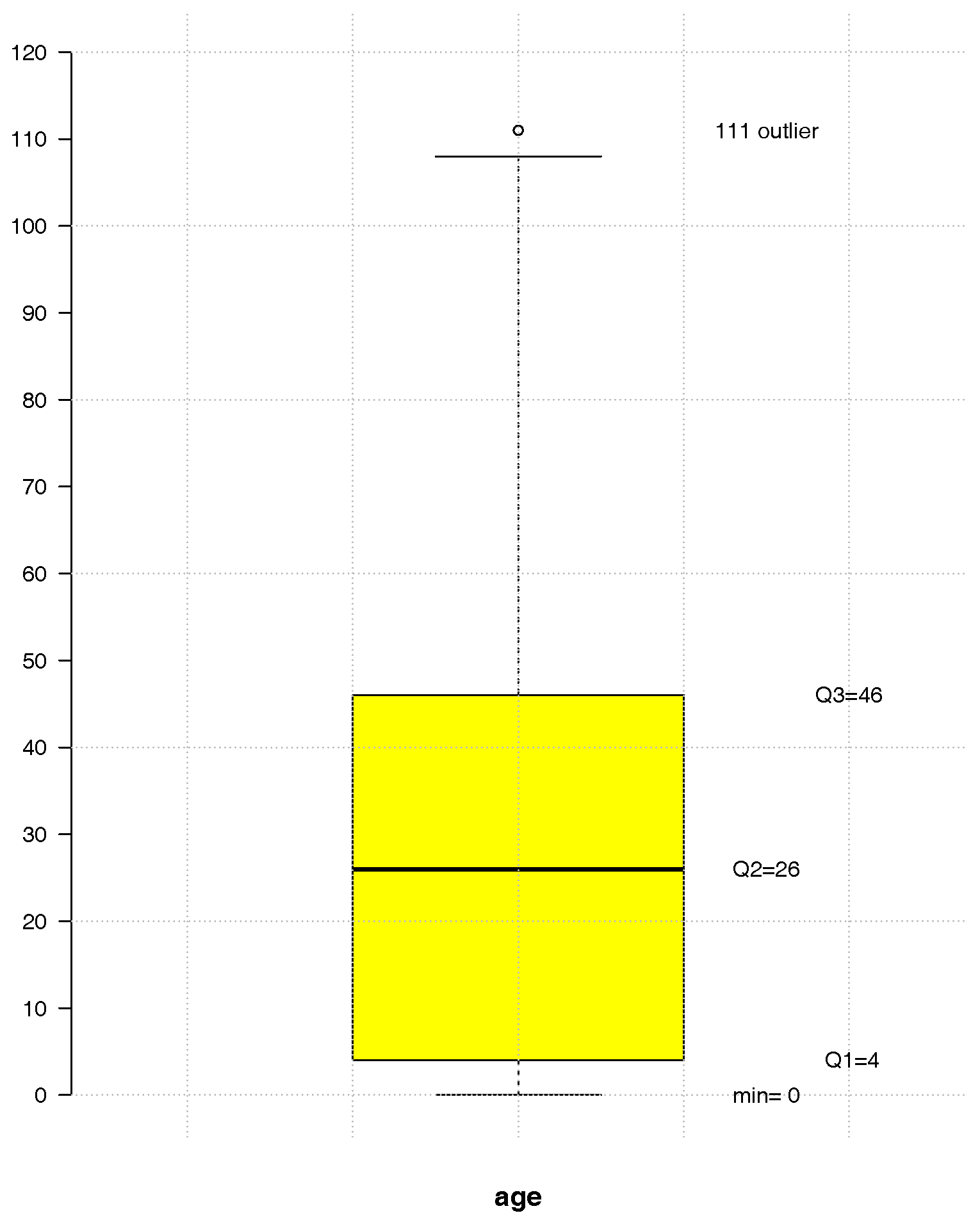
This work focuses on the number of TAE calls to LS24 in 2014 at a municipality level, in Continental Portugal. For this year, 50% of the users were aged between 4 and 46, with a median of 26 years and a range of 111 years—see Figure 1.
The distribution of the number of TAE calls to LS24, by municipality in 2014, is mapped in Figure 2. The average raw call rate by municipality is 32 per 1000 inhabitants.
3.2. Non-Spatial Modelling, the Log-Poisson Regression Model
The number of TAE calls to LS24 in each of the 278 municipalities of Continental Portugal were first modelled via a log-Poisson regression model before considering the need of a spatial analysis.
An indirect standardization of these numbers has been carried out, applied to the resident population of each municipality in terms of age groups, namely 0–9, 10–19, 20–29, 30–39, 40–49, 50–59, 60–69, 70–79 and >80. This method considers standard age rates
with the number of cases (calls) and the at risk population (resident population), in municipality i and age group j, , , in order to obtain , , the expected number of calls in each municipality, that is included in the model as an offset. So that, in fact, what is modelled is the relative call risk, which can be roughly estimated by the Standard Call Rate (SCR) mapped in Figure 3. This ratio is calculated from the observed number of cases and the expected number of cases, allowing comparisons across different populations. The resident population of each municipality in terms of age groups was obtained from Census 2011 data and adjusted for subsequent years (PORDATA-Database of Contemporary Portugal 2014).
Demographic and socio-economic information, development indicators as well as characteristics of the Portuguese health system at the municipal level, were investigated as possible covariates for modelling the TAE call counts in order to understand if the inclusion of certain covariates obviated the need for a spatial model. Using the Stepwise methodology of Rawlings et al. (1998) for selecting covariates, under different scenarios, the two best cases of the most significant sets of explanatory variables are:
- Case 1: The average number of years of schooling, the proportion of elderly residents, the unemployment rate, the rurality index, the number of hospitals and health centres per 1000 inhabitants and the proportion of women in each municipality (AIC: 29530);
- Case 2: The monthly average income, the proportion of children, the unemployment rate, the rurality index, the number of hospital and health centres (both per 1000 inhabitants), and the proportion of women in each municipality (AIC: 36980).
From these variables, the average number of years of schooling and the monthly average income are the ones that show a stronger positive correlation with the response variable (0.67 and 0.61, respectively), followed by the proportion of children (0.49). The rurality index and the proportion of elderly residents are negatively correlated with the response (−0.45 and −0.35, respectively).
Over-dispersion in these Poisson data is expected, as we suspect space to be an important feature for their modelling. If we ignore this over-dispersion, the standard errors of the covariate effects are underestimated, resulting in an incorrect assessment of the significance of individual regression parameters. Therefore, instead, we have opted to fit a quasi-Poisson model to account for the over-dispersion, realizing that the significant covariates under this approach were in fact different from the ones of the Poisson model (although the estimated effects are, of course, the same).
Table 1 and Table 2 depict the estimated coefficients of the considered quasi-Poisson log-regression models for these analyses, with
where is the relative risk in the ith municipality. For case 1, the unemployment rate turned out to be not significant after all, and for case 2, the same happened with the rurality index, the number of hospital and health centres.
3.3. Spatial Correlation
In this subsection standard spatial techniques are used to look for spatial dependence in the number of TAE calls, considering a contiguity neighbourhood structure, and also in the residuals of the log-Poisson regression models fitted before.
For the considered contiguity neighbourhood structure, the first order queen neighbourhood, there are 1.9% non-zero weights and the average number of neighbours is 5.3. Taking the corresponding queen neighbourhood matrix, and using Moran’s I statistics (1), for two sided test, both under normality (, ) or considering a randomized distribution of the statistics (, ), resulted in a clear rejection of the spatial independence hypothesis of the number of TAE calls, suggesting that there is a positive spatial correlation among these.
The spatial autocorrelation in the residuals of the log-Poisson regression models fitted in Section 3.2 was further investigated, using a randomized distribution of the statistic and a two sided test, having () for model 1 and () for model 2. The results suggest a high positive spatial autocorrelation in the residuals. With spatially correlated residuals, the fitted models may be providing biased estimates of the parameters, leading to incorrect interpretations and misleading conclusions (Lesage 1999). It is then clear that space is an important feature of these data and that must be considered in the modelling.
Package spdep (Bivand et al. 2014b) of R-project software was used to obtain the results presented in this section according to (Anselin 2007).
3.4. Spatial Modelling
3.4.1. Spatial Hierarchical Log-Poisson Regression Model
In order to capture and model data spatial variability, the number of TAE calls in each municipality is now analysed through different hierarchical log-Poisson regression models. The residual autocorrelation of the log-Poisson regression model considered before can be explained, in a Bayesian setting, adding to the model’s predictor a set of spatially structured () random effects, considering the contiguity neighbourhood structure mentioned before. Additional unstructured random effects () can be considered, if needed. The prior distributions of the random effects define their structure, as described in Section 2.2.
The estimates were obtained via MCMC, implemented in R-package CARBayes (Lee 2013). A MCMC run of 1,000,000 iterations was made, discarding 50,000 burn-in iterations and thinning by 100, in order to reduce autocorrelation, resulting in 100,000 sample points.
Two models were considered differing on the way the random effects are included.
Model A: BYM model
The BYM CAR prior model, applied to both cases 1 and 2 in Section 3.2, is a log-Poisson regression model with the covariates considered significant before plus unstructured () and spatially structured random effects (). The results are summarised in Table 3 and Table 4.
Model B: Leroux model
This is a log-Poisson regression model with the covariates previously considered significant plus the random effects (Leroux CAR prior). The results are displayed in Table 5 for case 1 and in Table 6 for case 2.
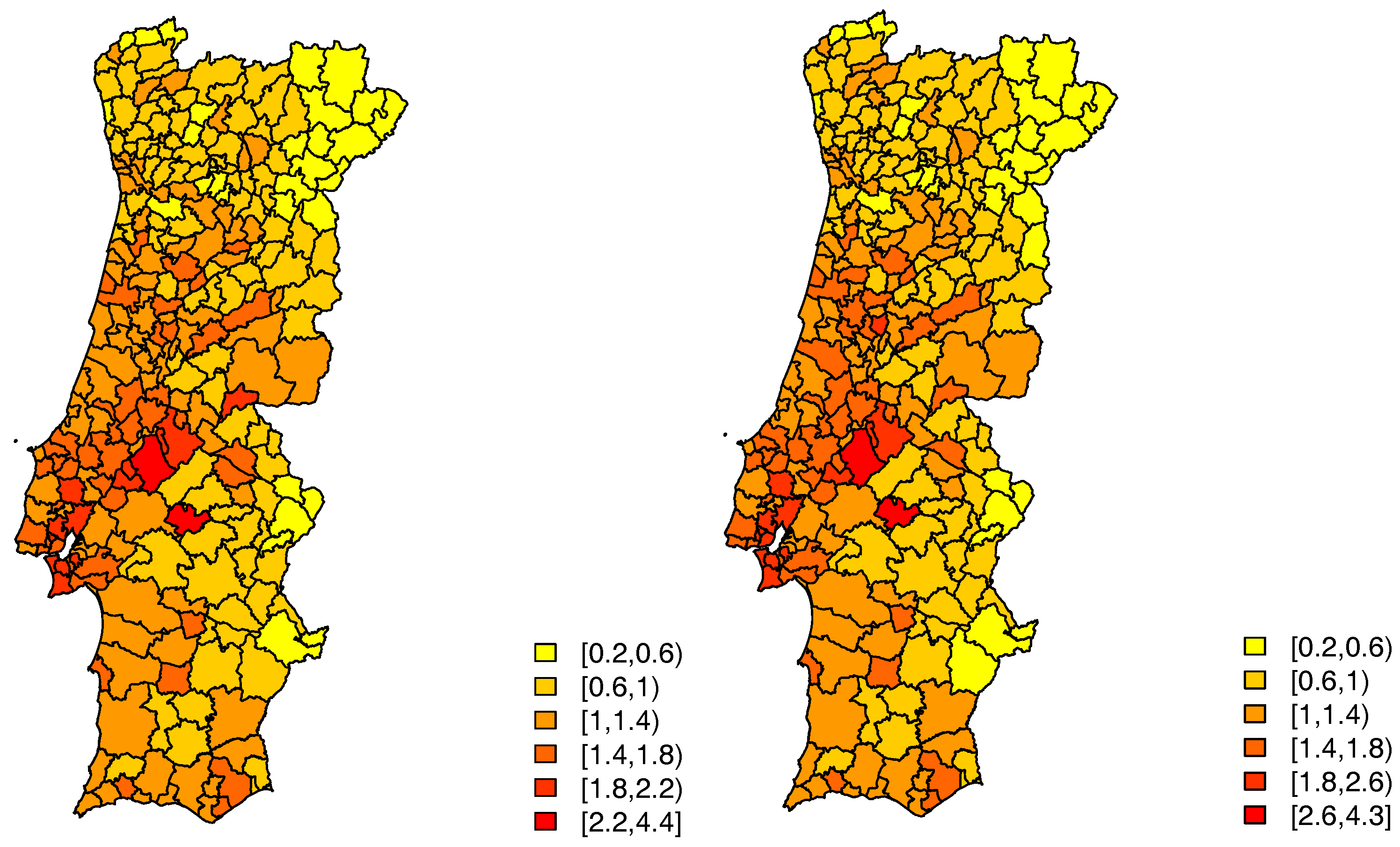
In this model, for the first case, only one of the initial covariates proved to be significant, the average number of years of schooling. The estimates of the random effects, given by , seem to indicate that there still is spatial variability in these data—right panel of Figure 4, which is strongly confirmed by an estimated value of of .
Considering this model, for the second case, also only one of the initial covariates proved to be significant, the monthly average income. This model has an estimated value of of , and the estimates of the random effects seem to indicate that there still is spatial variability—right panel of Figure 5.
3.4.2. The Spatial Lag Poisson Model
A modelling alternative is to account for spatial autocorrelation in the observed responses instead of the disturbances, as before, using an autoregressive perspective. This approach may also be considered for these data, given that it is plausible to think that the number of TAE calls to LS24 in one municipality is related to the number of calls in the municipalities of its neighbourhood, driven by effects of covariates such as the number of hospitals in one municipality, which may certainly have an impact on the number of calls to LS24 in a neighbour municipality, or others not considered in the modelling. Additionally, the considered covariates themselves display a high spatial dependency. Therefore, the response variable in a given area is most certainly a good predictor of the response variable in its neighbourhood areas.
Here, the TAE number of calls in each municipality is then analysed through the spatial lag Poisson model where a spatial autocorrelation lag is incorporated in the econometric model of counts. The estimates were obtained via INLA methodology, in terms of the “splmINLA” model, in R-package R-INLA, according to the R-code presented in Appendix B.
Model C: Spatial lag Poisson model
This is the spatial lag Poisson Bayesian autoregressive model with the covariates initially considered significant. Table 7 and Table 8 summarize the parameter estimates for case 1 and case 2, respectively.
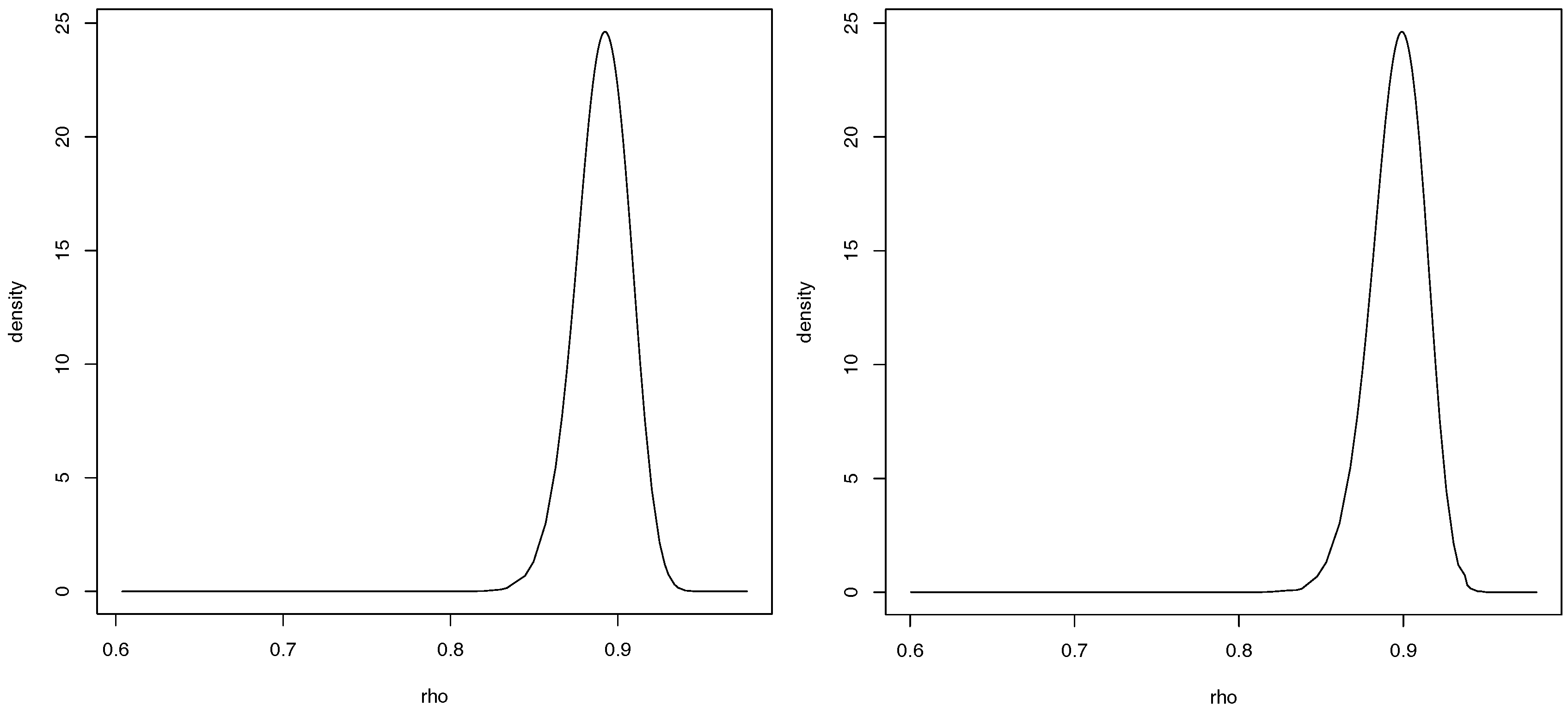
For case 1 only one of the previous covariates proved to be significant, the average number of years of schooling. This model has an estimated value of of . As for the second case, only the monthly average income is significant. This second model has an estimated value of of . The posterior marginal distribution of the spatial autocorrelation parameter, for both cases, is presented in Figure 6.
3.5. Comparison of Results
In the various spatial fits, the covariates considered important for explaining the number of calls and the corresponding effects where the same. These fits were further compared by means of their predictive accuracy, using the DIC measure and the WAIC measure. See Table 9 for case 1 and Table 10 for case 2. The Relative Root Mean Square Error (RRMSE) was also considered to measure goodness-of-fit. Results are displayed in Table 11 and Table 12.
In terms of spatial hierarchical log-Poisson regression models, the model with smaller DIC (preferred model) is the one including the covariates and the spatially structured random effects through Leroux CAR prior. This was confirmed by the RRMSE values. For the sake of comparison, the fit measures for the baseline log-Poisson regression model without random effects, also fitted by MCMC, are further displayed in the first line of the tables. The log-Poisson regression model was also fitted, including only covariates and unstructured random effects (results not shown here), which performed worse, indicating that spatial random effects are indeed necessary in the models. This might indicate that there are possibly some relevant covariates that are not yet being included in the model. There is a spatial asymmetry that is not explained by the variables. Similar conclusions were reached when the autoregressive perspective was considered in terms of the spatial lag Bayesian Poisson model.
In order to compare both hierarchical and autoregressive model fits, WAIC measure was used, as it is more appropriate for comparing different model structures. The autoregressive model reveals better performance, according to this measure. As for the RRMSE values, they are very similar although they are somewhat smaller for the hierarchical Leroux model.
4. Discussion
This study combines insights from classical spatial econometrics and the analysis of spatial data in order to handle spatial count data, both in a spatial hierarchical and in a spatial autoregressive perspectives. The approach applied here allows the limitations of the classical econometrics methods to be circumvented. In terms of the practical application, it represents a work in progress and this paper displays the first results of the proposed study.
Within the scope of the spatial econometric methods and also resorting to Bayesian hierarchical and autoregressive methodology, their application to study of the number of TAE calls to the national health line, LS24, revealed spatial-correlation and the addition of spatial structure in the models improved estimation.
In this study, the count data were first analysed with a log-Poisson regression model and then the inclusion of spatial random effects in a hierarchical Bayesian setting, proved to be relevant, as expected, although the modelling may perhaps be improved by considering some other more adequate covariates. Furthermore a recent alternative for doing Bayesian inference using INLA (Rue et al. 2009) for spatial econometric models, the slmINLA recently developed by Goméz-Rubio et al. (2015) and implemented in R-INLA, was explored. Subsequently, considering a multiplicative spatial autoregressive lag model for counts developed by Lambert et al. (2010), combined with the slmINLA model, a spatial lag Poisson model was developed, an alternative to do Bayesian inference for spatial econometric models for count data. Similar conclusions were drawn when both the hierarchical and the autoregressive perspectives were considered.
The average number of years of schooling for case 1 of the analysis and the average monthly income for case 2 stand out as being important in explaining the use of LS24. Additionally, the spatial component for both cases was quite relevant, which was confirmed by the high values of the estimates of the spatial autocorrelation parameter.
For the future it is the intention to proceed with the study of the LS24 data set, maybe considering some other possible relevant covariates and to carry out analyses under other possible scenarios in order to be able to describe and evaluate in which municipalities the use of LS24 should be encouraged, as well as detecting those regions that most contribute to the economic success of the good use of the line for future assessment of hospital savings (Hughes and McGuire 2003).
Additionally, this analysis should be extended to include available data for previous years between 2010 and 2014, fitting some spatio-temporal models (Cressie and Wikle 2011) under an econometric approach and developing and implementing the temporal effects on Bayesian hierarchical models (Banerjee et al. 2004; Lee et al. 2015), or on Bayesian autoregressive models (Blangiardo and Cameletti 2015), for count data, trending towards a spatio-temporal Bayesian econometric approach for processing count data. It is expected that analyses like the one considered here for the LS24 data contribute, in general, to the improvement of management policies in several areas of activity, the hospital domain in this case, or in others such as education or road safety.
Acknowledgments
This work is financed by national funds through FCT—Foundation for Science and Technology—under the projects UID/MAT/00297/2013 and UID/MAT/00006/2013. The authors thank the Referees for their careful and detailed revision of this paper, which has greatly improved the work.
Author Contributions
Paula Simões, M. Lucília Carvalho and Isabel Natário, reviewed, discussed and developed the proposed methodologies for the specific Poisson data type; Paula Simõe analysed the data and implemented this study in the R software; Paula Simões, M. Lucília Carvalho, Sandra Aleixo and Isabel Natário wrote the paper and Sérgio Gomes collected and made available the L24 data.
Conflicts of Interest
The authors declare no conflict of interest. The founding sponsors had no role in the design of the study; in the collection, analyses, or interpretation of data; in the writing of the manuscript, and in the decision to publish the results.
Abbreviations
The following abbreviations are used in this manuscript:
| LS24 | Portuguese national health line |
| slm | spatial autoregressive model |
| sem | spatial error model |
| MCMC | Markov Chain Monte Carlo |
| INLA | Integrated Nested Laplace Approximations |
| CAR | Conditional autoregressive |
| GMRF | Gaussian Markov Random Field |
| BYM | Besag-York-Mollié |
| slmINLA | spatial lag model |
| splmINLA | spatial lag Poisson model |
| AIC | Akaike information criteria |
| DIC | Deviance information criteria |
| WAIC | Watanabe-Akaike information criteria |
| TAE | Triage, counseling and routing |
| AT | Therapeutic counseling |
| LSP | Assistance in Public Health |
| IGS | General Health Information |
| SCR | Standard Call Rate |
| RRMSE | Relative Root Mean Square Error |
| MVN | Multivariate Normal |
Appendix A. The Integrated Nested Laplace Approximation
Recently Rue et al. (2009) have developed an approximate method, known as the Integrated Nested Laplace Approximation (INLA), that allows one to estimate the marginal posterior distribution of the parameters of interest in a Bayesian model, being particularly efficient in the estimation of latent Gaussian models and capable of providing accurate and fast results (Blangiardo and Cameletti 2015; Rue et al. 2009). Another advantage is that it is quit general in the type of model that it can fit, allowing for great automation of the inferential process. Nowadays this method is available through program R, with package R-INLA. Next are described the INLA methodology and the corresponding context in which it should be applied, according to Blangiardo and Cameletti (2015) and Natário (2013).
Consider n observed values of our response variable, , that are assumed to be distributed according to one of the distributions in the exponential family, with mean parameter , related to the linear predictor through a link function :
This linear predictor is defined as:
where is a scalar that represents the intercept, corresponds to the linear effects of the chosen covariates on the response, and to the non-linear effects, functions of the variables .
The class of Gaussian models is very flexible, the terms can assume many different forms as non-linear effects of covariates, seasonal effects, temporal or spatial random effects, covering generalized linear models, hierarchical models, spatial and spatio-temporal models. The vector of latent effects, forms a Gaussian Markov Random Field (GMRF) with precision matrix , where is also a vector of hyperparameters. The distribution of will depend on a number of parameters . Consider the density function of , assuming conditional independence given and , the distribution of the n observations is given by,
Let be a single vector of parameters, with density function . The posterior distribution of the latent effects, , and the parameters , with precision matrix ) is given by,
corresponding to the product of the likelihood (A2), of the GMFR prior density and the parameter prior distribution .
The INLA approach does not estimate the posterior marginal distributions of the latent effects, , and the hyperparameters , but rather the whole posterior distribution,
by constructing “nested approximations”, numerical approximations based on the Laplace approximation method. This method allows one to approximate the density function by the first terms of Taylor series expansion of the log of the density.
where corresponds to the approximate density function. The proposed Laplace approximation for is then given by,
where is the Gaussian approximation, given by the Laplace approximation method, where , and is the mode for a given .
The INLA approximation of follows three main steps:
- i
- Computation of an approximation to the posterior distribution of the hyperparameters as in (A4),
- ii
- Use again the Laplace approximation to obtain . For example, rewriting the vector of parameters as ,where is the mode.
- iii
- Using the previous steps and a numerical integration,can be solved through a finite weighted sum:considering that , has m relevant elements with a corresponding set of weights , where m small.
Appendix B. R-Code Used in R-INLA to Implement Spatial Lag Poisson Model
Start with the R-Code available in http://www.math.ntnu.no/inla/r-inla.org/doc/latent/slm.pdf for fitting the slmINLA model:
#### slmINLA Model:

## Index for the latent model
BD3$idx

## Define adjacency using a row-standardised matrix
concelhos_listw<-nb2listw(concelhos_nb)
W <- as(as_dgRMatrix_listw(concelhos_listw), "CsparseMatrix")

## Model definition log_n.cham_pop.resi/log.cham.SMR
f1 <- log.cham.SMR ~Escolaridade + Perc.idosos+TxDesemp+IndRural+
  +Hospitais1000+CentrosSaude1000+ PropMulheres

f2 <- log.cham.SMR ~Perc.criancas + TxDesemp+Rendim+IndRural +
  +Hospitais1000+CentrosSaude1000+ PropMulheres

#Covariate matrix###
mmatrix1 <- model.matrix(f1,BD3)
mmatrix2<- model.matrix(f2,BD3)

## Zero-variance for error term
zero.variance = list(prec=list(initial = 25, fixed=TRUE))


## Compute eigenvalues for slm model, used to obtain rho.min and
## rho.max
e = eigenw(concelhos_listw)
re.idx = which(abs(Im(e)) < 1e-6)
rho.max = 1/max(Re(e[re.idx]))
rho.min = 1/min(Re(e[re.idx]))
rho = mean(c(rho.min, rho.max))

## Precision matrix for beta coeffients’ prior
betaprec <- .0001
Q.beta = Diagonal(n=ncol(mmatrix), betaprec)

## Priors on the hyperparameters
hyper = list(
  prec = list(
    prior = "loggamma",
    param = c(0.01, 0.01)),
  rho = list(
    initial=0,
    prior = "logitbeta",
    param = c(1,1)))

    Next, there is the R-code for fitting the spatial lag poisson model:


## slpmINLA Model
## Fit model  for SCR case1
slmm1 <- inla( n.chamadas ~ -1 +
                 f(idx, model="slm",
                   args.slm=list(
                     rho.min = rho.min,
                     rho.max = rho.max,
                     W=W,
                     X=mmatrix1,
                     Q.beta=Q.beta),
                   hyper=hyper),
               data=BD3, family="poisson",
               control.family = list(hyper=zero.variance),
               control.compute=list(dic=TRUE, cpo=TRUE, waic=TRUE),
               offset=log(e_st)
)

n <- nrow(BD3)
slmm1$summary.random$idx[n+1:ncol(mmatrix1),]

## Fit model for SCR case2

slmm2 <- inla( n.chamadas ~ -1 +
                 f(idx, model="slm",
                   args.slm=list(
                     rho.min = rho.min,
                     rho.max = rho.max,
                     W=W,
                     X=mmatrix2,
                     Q.beta=Q.beta),
                   hyper=hyper),
               data=BD3, family="poisson",
               control.family = list(hyper=zero.variance),
               control.compute=list(dic=TRUE, cpo=TRUE, waic=TRUE),
               offset=log(e_st)
)

n <- nrow(BD3)
slmm2$summary.random$idx[n+1:ncol(mmatrix2),]
References
- Anselin, Luc. 2007. Spatial Regression Analysis in R—A Workbook. Urbana: Center for Spatially Integrated Social Sciences. [Google Scholar]
- Anselin, Luc. 2010. Thirty Years of Spatial Econometrics. Papers in Regional Science 89: 3–25. [Google Scholar] [CrossRef]
- Anselin, Luc, Anil K. Bera, Raymond Florax, and Mann J. Yoon. 1996. Simple diagnostic tests for spatial dependence. Regional Science and Urban Economics 26: 77–104. [Google Scholar] [CrossRef]
- Arbia, Giuseppe. 2006. Spatial Econometrics: Statistical Foundations and Applications to Regional Convergence. Heidelberg and Berlin: Springer. [Google Scholar]
- Banerjee, Sudipto, Bradley P. Carlin, and Alan E. Gelfand. 2004. Hierarchical Modeling and Analysis for Spatial Data. Boca Raton: Chapman and Hall/CRC. [Google Scholar]
- Besag, Julian. 1974. Spatial Interaction and the Statistical Analysis of Lattice Systems (with discussion). Journal of the Royal Statistical Society B 36: 192–236. [Google Scholar]
- Besag, Julian, Jeremy York, and Annie Mollié. 1991. Bayesian image restoration with two applications in spatial statistics (with discussion). Annals of The Institute of Statistical Mathematics 43: 1–59. [Google Scholar] [CrossRef]
- Bivand, Roger S., Virgilio Goméz-Rubio, and Havard Rue. 2014a. Approximate Bayesian inference for spatial econometrics models. Spatial Statistics 9: 146–65. [Google Scholar] [CrossRef]
- Bivand, Roger, Micah Altman, Luc Anselin, Renato Assunção, Olaf Berke, Andrew Bernat, Guillaume Blanchet, Eric Blankmeyer, Marilia Carvalho, Bjarke Christensen, and et al. 2014b. Spdep: Spatial Dependence: Weighting Schemes, Statistics and Models. Available online: http://cran.r-project.org/web/packages/spdep/index.html (accessed on 1 February 2016).
- Blangiardo, Marta, and Michela Cameletti. 2015. Spatial and Spatial-Temporal Bayesian Models with R-INLA. Chichester: Wiley. [Google Scholar]
- Carvalho, M. Lucília, and Isabel Natário. 2008. Análise de Dados Espaciais. Lisboa: Sociedade Portuguesa de Estatística. [Google Scholar]
- Cressie, Noel A. C. 1993. Statistics for Spatial Data. New York: Jonh Wiley & Sons, Inc. [Google Scholar]
- Cressie, Noel A. C., and Christopher K. Wikle. 2011. Statistics for Spatio-Temporal Data. Hoboken: Jonh Wiley & Sons, Inc. [Google Scholar]
- Dass, Sarat C., Chae Young Lim, and Tapabrata Maiti. 2010. Experiences with Aproximate Bayes Inference for the Poisson-CAR Model. Techinal Report RM679. East Lansing: Department of Statistics and Probability, Michigan State University. [Google Scholar]
- Database of Contemporary Portugal. 2014. Available online: https://www.pordata.pt/ (accessed on 3 April 2016).
- Doucet, Arnaud, Nando de Freitas, and Neil Gordon, eds. 2001. Sequential Monte Carlo Methods in Practice. New York: Springer. [Google Scholar]
- Fischer, Manfred M. 2006. Spatial Analysis and GeoComputation. Heidelberg and Berlin: Springer. [Google Scholar]
- Gelman, Andrew, Jessica Hwang, and Aki Vehtari. 2014. Understanding predictive information criteria for Bayesian models. Statistics and Computing 24: 997–1016. [Google Scholar] [CrossRef]
- Goméz-Rubio, Virgilio, Roger S. Bivand, and Havard Rue. 2015a. A new latent class to fit spatial econometrics models with Integrated Nested Laplace Approximations. In Spatial Statistics: Emmerging Patterns—Part 2. vol. 27, pp. 116–18. Available online: http://www.math.ntnu.no/inla/r-inla.org/doc/latent/slm.pdf (accessed on 21 September 2016).
- Goméz-Rubio, Virgilio, Roger S. Bivand, and Havard Rue. 2015b. Estimating Spatial Econometrics Models with Integrated Nested Laplace Approximations. Technical Report-Preprint to Elsevier. Available online: https://previa.uclm.es/profesorado/vgomez/SSTMR/papers/INLA-slm.pdf (accessed on 27 June 2016).
- Hughes, David, and Alistair McGuire. 2003. Stochastic demand, production responses and hospital costs. Journal of Health Economics 22: 999–1010. [Google Scholar] [CrossRef]
- Lambert, Dayton M., Jason P. Brown, and Raymond J. G. M. Florax. 2010. A two-step estimator for a spatial lag model of counts: Theory, small sample performance and an application. Regional Science and Urban Economics 40: 241–52. [Google Scholar] [CrossRef]
- Lee, Duncan. 2013. R Archive Network: CARBayes. CRAN. Available online: https://cran.r-project.org/web/packages/CARBayes/ (accessed on 3 February 2016).
- Lee, Duncan. 2014. CARBayes: An R Package for Bayesian Spatial Modeling with Conditional Autoregressive Priors. Journal of Statistical Software 55, Issue 13. [Google Scholar] [CrossRef]
- Lee, Duncan, Alastair Rushworth, and Gary Napier. 2015. CARBayesST: An R Package for Spatio-temporal Areal Unit Modelling with Conditional Autoregressive Priors. R Package Version 2.2. Available online: https://cran.r-project.org/web/packages/CARBayesST/ (accessed on 25 February 2016).
- Leroux, Brian G., Xingye Lei, and Norman Breslow. 1999. Estimation of Disease Rates in Small Areas: A New Mixed Model for Spatial Dependence. In Statistical Models in Epidemiology, the Environment, and Clinical Trials. Edited by M. E. Halloran and D. Berry. New York: Springer, pp. 135–78. [Google Scholar]
- Lesage, James P. 1999. The Theory and Practice of Spatial Econometrics. Toledo: University of Toledo. [Google Scholar]
- Lesage, James P., and Robert Kelley Pace. 2009. Introduction to Spatial Econometrics. Boca Raton: CRC Press. [Google Scholar]
- Natário, Isabel. 2013. Métodos Computacionais: INLA, Integrated Nested Laplace Approximation. Boletim da Sociedade Portuguesa de Estatística Outono de 2013: 52–56. [Google Scholar]
- Portal of the National Portuguese Health Service. 2015. Available online: https://www.dgs.pt/paginas-de-sistema/saude-de-a-a-z/saude-24.aspx (accessed on 3 September 2015).
- Quddus, Mohammed A. 2008. Modelling area-wide count outcomes with spatial correlation and heterogeneity: An analysis of London crash data. Accident Analysis and Prevention 40: 1486–97. [Google Scholar] [CrossRef] [PubMed]
- Rawlings, John O., Sastry G. Pantula, and David A. Dickey. 1998. Applied Regression Analysis: A Research Tool, 2nd ed. New York: Springer. [Google Scholar]
- Rue, Havard, Sara Martino, and Nicolas Chopin. 2009. Approximate Bayesian inference for lattent Gaussian models by using integreted nested Laplace approximations. Journal of the Royal Statistical Society: Series B 71, Part 2: 319–92. [Google Scholar] [CrossRef]
- Spiegelhalter, David J., Nicola G. Best, Bradley P. Carlin, and Angelika Van der Linde. 2002. Bayesian Measures of Model Complexity and Fit. Journal of the Royal Statistical Society B 64: 583–639. [Google Scholar] [CrossRef]
- Stern, Hal, and Noel A. Cressie. 1999. Inference for Extremes in Disease Mapping. In Disease Mapping and Risk Assessment for Public Health. Edited by Andrew B. Lawson, Annibale Biggeri, Dankmar Böhning, Emmanuel Lesaffre, Jean-Fran Viel and Roberto Bertollini. Hoboken: John Wiley & Sons, pp. 63–84. [Google Scholar]
- Vehtari, Aki, Andrew Gelman, and Jonah Gabry. 2017. Pratical Bayesian model evaluation using leave-one-out cross-validation and WAIC. Statistics and Computing 27: 1413–32. [Google Scholar] [CrossRef] [PubMed]
- Watanabe, Sumio. 2010. Asymptotic equivalence of Bayes cross-validation and widely applicable information criterion in singular learning theory. Journal of Machine Learning Research 11: 3571–94. [Google Scholar]
Figure 1.
The LS24 users age empirical distribution in 2014.

Figure 2.
Number of TAE calls to LS24 per 1000 inhabitants, in 2014.
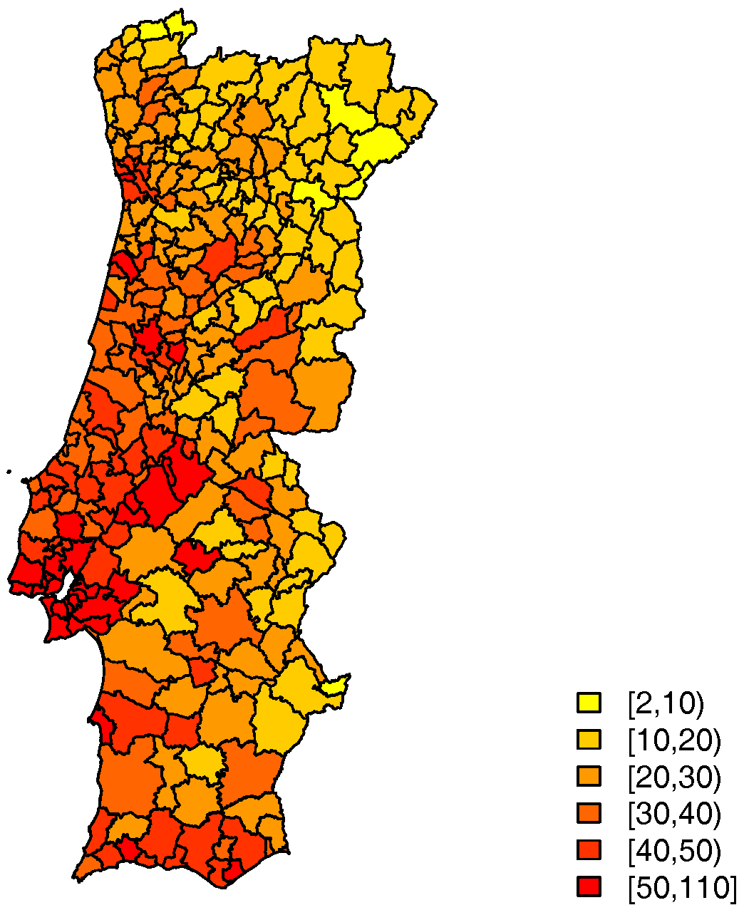
Figure 3.
Standard Call Rate to LS24, in 2014.

Figure 4.
Estimated random effects for Model A (Left) and for Model B (Right), case 1.

Figure 5.
Estimated random effects for Model A (Left) and for Model B (Right), case 2.
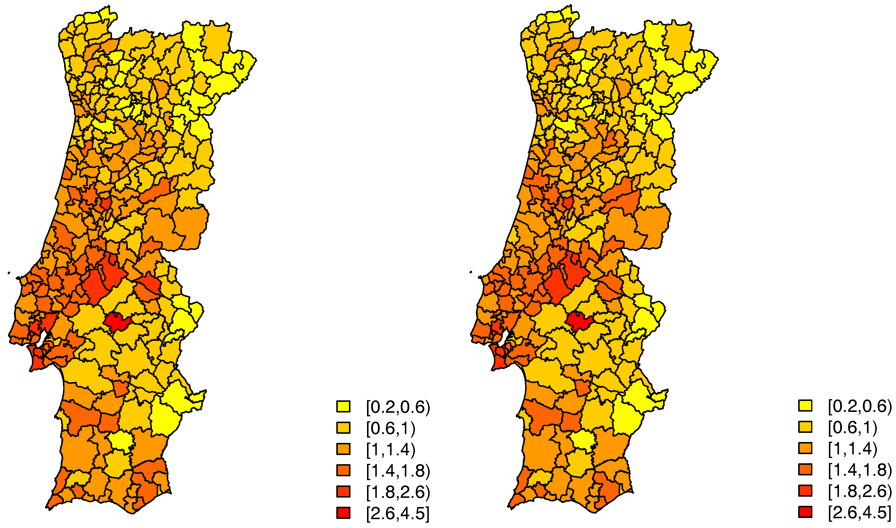
Figure 6.
Posterior marginal distribution of the spatial autocorrelation parameter for Model C, case 1 (Left) and case 2 (Right).
Figure 6.
Posterior marginal distribution of the spatial autocorrelation parameter for Model C, case 1 (Left) and case 2 (Right).

Table 1.
Covariates and their estimated coefficients for the quasi-Poisson log-regression model, case 1, for the LS24 2014 data.
Table 1.
Covariates and their estimated coefficients for the quasi-Poisson log-regression model, case 1, for the LS24 2014 data.
| Variable | Id | Coefficients | p-Values |
|---|---|---|---|
| Average number of years of schooling | <2 | ||
| Proportion of elderly residents | 9.52 | ||
| Unemployment rate | 0.3156 | ||
| Rurality index | 4.10 | ||
| Number of hospitals | 6.68 | ||
| Number of health centres | 0.0437 | ||
| Proportion of women | 0.0661 | ||
| Intercept | 0.8390 |
Table 2.
Covariates and their estimated coefficients for the quasi-Poisson log-regression model, case 2, for the LS24 2014 data.
Table 2.
Covariates and their estimated coefficients for the quasi-Poisson log-regression model, case 2, for the LS24 2014 data.
| Variable | Id | Coefficients | p-Values |
|---|---|---|---|
| The monthly average income | 5.97 | ||
| Proportion of children | 0.0004 | ||
| Unemployment rate | 0.0391 | ||
| Rurality index | 0.1884 | ||
| Number of hospitals | 0.6504 | ||
| Number of health centres | 0.1702 | ||
| Proportion of women | 0.0003 | ||
| Intercept | 7.64 |
Table 3.
Parameter estimates for the Besag, York and Mollié (BYM) hierarchical log-Poisson model, case 1, for the LS24 2014 data.
Table 3.
Parameter estimates for the Besag, York and Mollié (BYM) hierarchical log-Poisson model, case 1, for the LS24 2014 data.
| Variable | Id | Median | 2.5% | 97.5% |
|---|---|---|---|---|
| Average number of years of schooling | ||||
| Proportion of elderly residents | ||||
| Unemployment rate | ||||
| Rurality index | ||||
| Number of hospitals | ||||
| Number of health centres | ||||
| Proportion of women | ||||
| Intercept | ||||
Table 4.
Parameter estimates for the BYM hierarchical log-Poisson model, case 2, for the LS24 2014 data.
Table 4.
Parameter estimates for the BYM hierarchical log-Poisson model, case 2, for the LS24 2014 data.
| Variable | Id | Median | 2.5% | 97.5% |
|---|---|---|---|---|
| The monthly average income | ||||
| Proportion of children | ||||
| Unemployment rate | ||||
| Rurality index | ||||
| Number of hospitals | ||||
| Number of health centres | ||||
| Proportion of women | ||||
| Intercept | ||||
Table 5.
Parameter estimates for the Leroux hierarchical log-Poisson model, case 1, for the LS24 2014 data.
Table 5.
Parameter estimates for the Leroux hierarchical log-Poisson model, case 1, for the LS24 2014 data.
| Variable | Id | Median | 2.5% | 97.5% |
|---|---|---|---|---|
| Average number of years of schooling | ||||
| Proportion of elderly residents | ||||
| Unemployment rate | ||||
| Rurality index | ||||
| Number of hospitals | ||||
| Number of health centres | ||||
| Proportion of women | ||||
| Intercept | ||||
Table 6.
Parameter estimates for the Leroux hierarchical log-Poisson model, case 2, for the LS24 2014 data.
Table 6.
Parameter estimates for the Leroux hierarchical log-Poisson model, case 2, for the LS24 2014 data.
| Variable | Id | Median | 2.5% | 97.5% |
|---|---|---|---|---|
| The monthly average income | ||||
| Proportion of children | ||||
| Unemployment rate | ||||
| Rurality index | ||||
| Number of hospitals | ||||
| Number of health centres | ||||
| Proportion of women | ||||
| Intercept | ||||
Table 7.
Parameter estimates for the Spatial lag Poisson model, case 1, for the LS24 2014 data.
| Variable | Id | Median | 2.5% | 97.5% |
|---|---|---|---|---|
| Average number of years of schooling | ||||
| Proportion of elderly residents | ||||
| Unemployment rate | ||||
| Rurality index | ||||
| Number of hospitals | ||||
| Number of health centres | ||||
| Proportion of women | ||||
| Intercept | ||||
Table 8.
Parameter estimates for the Spatial lag Poisson model, case 2, for the LS24 2014 data.
| Variable | Id | Median | 2.5% | 97.5% |
|---|---|---|---|---|
| The monthly average income | ||||
| Proportion of children | ||||
| Unemployment rate | ||||
| Rurality index | ||||
| Number of hospitals | ||||
| Number of health centres | ||||
| Proportion of women | ||||
| Intercept | ||||
Table 9.
Deviance Information Criterion (DIC) and Watanabe-Akaike Information Criterion (WAIC) measured for the 3 models fitted for case 1.
Table 9.
Deviance Information Criterion (DIC) and Watanabe-Akaike Information Criterion (WAIC) measured for the 3 models fitted for case 1.
| Model | DIC | pD | WAIC | pW |
|---|---|---|---|---|
| Baseline Model MCMC | 2816.9 | 287.2 | 2830.8 | 198.5 |
| Model A | 2801.1 | 275.2 | 2773.8 | 179.9 |
| Model B | 2788.6 | 267.16 | 2744.5 | 157.2 |
| Model C | 2778.63 | 261.96 | 2717.6 | 144.9 |
Table 10.
DIC and WAIC measured for the 3 models fitted for case 2.
| Model | DIC | pD | WAIC | pW |
|---|---|---|---|---|
| Baseline Model MCMC | 2816.9 | 287.2 | 2830.8 | 198.5 |
| Model A | 2800.0 | 275.6 | 2770.7 | 169.5 |
| Model B | 2793.2 | 272.4 | 2743.0 | 156.7 |
| Model C | 2777.3 | 262.6 | 2714.1 | 143.8 |
Table 11.
Relative Root Mean Square Error (RRMSE) measured for the 3 models fitted for case 1.
| Model | RRMSE |
|---|---|
| Baseline Model | 0.588 |
| Model A | 0.029 |
| Model B | 0.028 |
| Model C | 0.037 |
Table 12.
RRMSE measured for the 3 models fitted for case 2.
| Model | RRMSE |
|---|---|
| Baseline Model | 0.469 |
| Model A | 0.025 |
| Model B | 0.026 |
| Model C | 0.034 |
© 2017 by the authors. Licensee MDPI, Basel, Switzerland. This article is an open access article distributed under the terms and conditions of the Creative Commons Attribution (CC BY) license (http://creativecommons.org/licenses/by/4.0/).
Share and Cite
MDPI and ACS Style
Simões, P.; Carvalho, M.L.; Aleixo, S.; Gomes, S.; Natário, I. A Spatial Econometric Analysis of the Calls to the Portuguese National Health Line . Econometrics 2017, 5, 24. https://doi.org/10.3390/econometrics5020024
AMA Style
Simões P, Carvalho ML, Aleixo S, Gomes S, Natário I. A Spatial Econometric Analysis of the Calls to the Portuguese National Health Line . Econometrics. 2017; 5(2):24. https://doi.org/10.3390/econometrics5020024
Chicago/Turabian StyleSimões, Paula, M. Lucília Carvalho, Sandra Aleixo, Sérgio Gomes, and Isabel Natário. 2017. "A Spatial Econometric Analysis of the Calls to the Portuguese National Health Line " Econometrics 5, no. 2: 24. https://doi.org/10.3390/econometrics5020024
Note that from the first issue of 2016, this journal uses article numbers instead of page numbers. See further details here.