
Oil Price and Economic Growth: A Long Story?


1
Department of Applied Economics, University of Zaragoza, Zaragoza 50006, Spain
2
Directorate General Economics, Statistics and Research, Bank of Spain, Madrid 28045, Spain
3
Department of Economic Analysis, University of Zaragoza, Zaragoza 50006, Spain
*
Author to whom correspondence should be addressed.
Econometrics 2016, 4(4), 41; https://doi.org/10.3390/econometrics4040041
Submission received: 30 August 2016
/
Revised: 30 September 2016
/
Accepted: 7 October 2016
/
Published: 28 October 2016
(This article belongs to the Special Issue Unit Roots and Structural Breaks)
Abstract
:This study investigates changes in the relationship between oil prices and the US economy from a long-term perspective. Although neither of the two series (oil price and GDP growth rates) presents structural breaks in mean, we identify different volatility periods in both of them, separately. From a multivariate perspective, we do not observe a significant effect between changes in oil prices and GDP growth when considering the full period. However, we find a significant relationship in some subperiods by carrying out a rolling analysis and by investigating the presence of structural breaks in the multivariate framework. Finally, we obtain evidence, by means of a time-varying VAR, that the impact of the oil price shock on GDP growth has declined over time. We also observe that the negative effect is greater at the time of large oil price increases, supporting previous evidence of nonlinearity in the relationship.
JEL Classification:
C22; C32; E32; Q431. Introduction
The literature on oil and macroeconomic variables is very extensive (see [1,2]). There is an ongoing debate on the interaction between oil price and macroeconomic performance. However, analyses of the link between oil price shocks and the business cycle have concentrated almost completely on relatively short horizons, from the early 1970s on. In particular, two specific periods have received a great deal of attention: the 1970s in particular and, to a lesser extent, the years since the beginning of the 21st century. It is well recognized that this interest dates back to the 1970s because the 1970s (and also the early 1980s) were characterized by serious oil price fluctuations together with unfavorable oil supply shocks, considered as the reasons behind worldwide macroeconomic volatility and stagflation. The interest has been rekindled in more recent times, given the possibility of a recurrence of this scenario. Indeed, some authors have investigated the different effects between these two periods on the macroeconomic variables see [3,4].1 Two notable exceptions to this relatively short-term perspective are [7], who investigate the volatility and persistence patterns of oil price shocks based on annual data for 1861–2008,2 and, more recently [8], who analyze the effects of oil prices on output and real dividends using a quarterly sample beginning in 1946.
The fact that the literature has focused on correctly identifying the source of shocks on oil prices, almost exclusively during the post-1970s period, is related to the frequent and tumultuous events in oil price markets at that time. It is also due to the absence of high-frequency data from earlier periods. However, much can be learned about the relationship between oil prices and macroeconomic conditions from the less-recent past. We expect that over such a long period there have been important changes in the demand and supply for oil that could lead to identify some structural breaks. For instance, prior to the mass production of automobiles, demand for oil focused on kerosene lamps. Regarding oil supply, the relative importance of Texas Railroad Commission and OPEC in setting world oil prices changed over this period. In this study, we aim to investigate changes in the behavior of oil prices and their influence on the US economy, using the longest available oil price series (January 1861–February 2016), which allows us to offer an alternative view to the literature of the historical role of the macroeconomic effects of oil.
The contributions of this study, which has some advantages over the previous literature, are twofold. First, we use data with a broader coverage in the time dimension than the previous studies (January 1861–February 2016 for oil prices and January 1875–February 2016 for GDP). In particular, our study is the first one, as far as we know, that captures the relationship between oil price shocks and the US GDP growth with such a long-term perspective. Second, we provide a comprehensive methodological framework to analyze the relationship between the two variables. We investigate the univariate properties of the series, focusing on the presence of structural breaks and volatility. Then, we adopt a multivariate perspective to delve into the relationship between oil price shocks and GDP performance in order to identify structural breaks in the multivariate regressions by employing three complementary tools: a VAR method, a rolling estimation of causality and long-term impacts, and the Qu and Perron (QP, henceforth) methodology [9]. Once the presence of instabilities in the series has been established, we propose a time-varying GDP-oil price model to capture the relationship between the two variables over time, detailing impulse responses during periods of intense shocks in the oil price markets.
The main findings of the study are as follows. First, although neither of the two series presents structural breaks in the mean, we identify in both of them, separately, different volatility periods associated with major events either in the economic performance of the US economy or in the oil markets. Second, delving deep into the relationship between the two variables through the full period, we observe that changes in oil prices have no significant effect on GDP growth. Nevertheless, it is reasonable to think that, with so many significant events in such a long period, both in business cycle dynamics and in the demand and supply factors of oil prices, the relationship between the two variables may have not been so stable. This is clear when we carry out a rolling analysis and investigate the presence of structural breaks in the multivariate framework. In particular, we clearly identify four different periods: February 1875–April 1912, January 1913–January 1941, February 1941–March 1970, and April 1970–February 2016. Third, we obtain evidence of a changing relationship over time regarding the time-varying VAR: the impact of an oil price shock on GDP growth has declined over time. We also observe that the negative effect is greater at the time of large oil price increases, supporting previous evidence of nonlinearity in the relationship.
The remainder of the paper is organized as follows. Section 2 describes the dataset used in the analysis. Section 3 investigates the univariate evolution of the series, focusing on the presence of structural breaks in mean and volatility. Section 4 analyzes the transmission of the effects between oil price shocks and GDP growth, adopting a multivariate perspective. Section 5 proposes a time-varying VAR model to capture different behaviors in the relationship over time. Finally, Section 6 concludes the study.
2. Data
We use series beginning in the nineteenth century and running until the present for our analysis of oil prices and US GDP. Regarding the US GDP, we use real quarterly data from the Bureau of Economic Analysis (BEA) and the National Bureau of Economic Research (NBER), covering the period January 1875 to February 2016. In particular, the BEA GDP series from 1947 onward is linked to a historical dataset beginning in 1875, which is available at the NBER until 1983.3
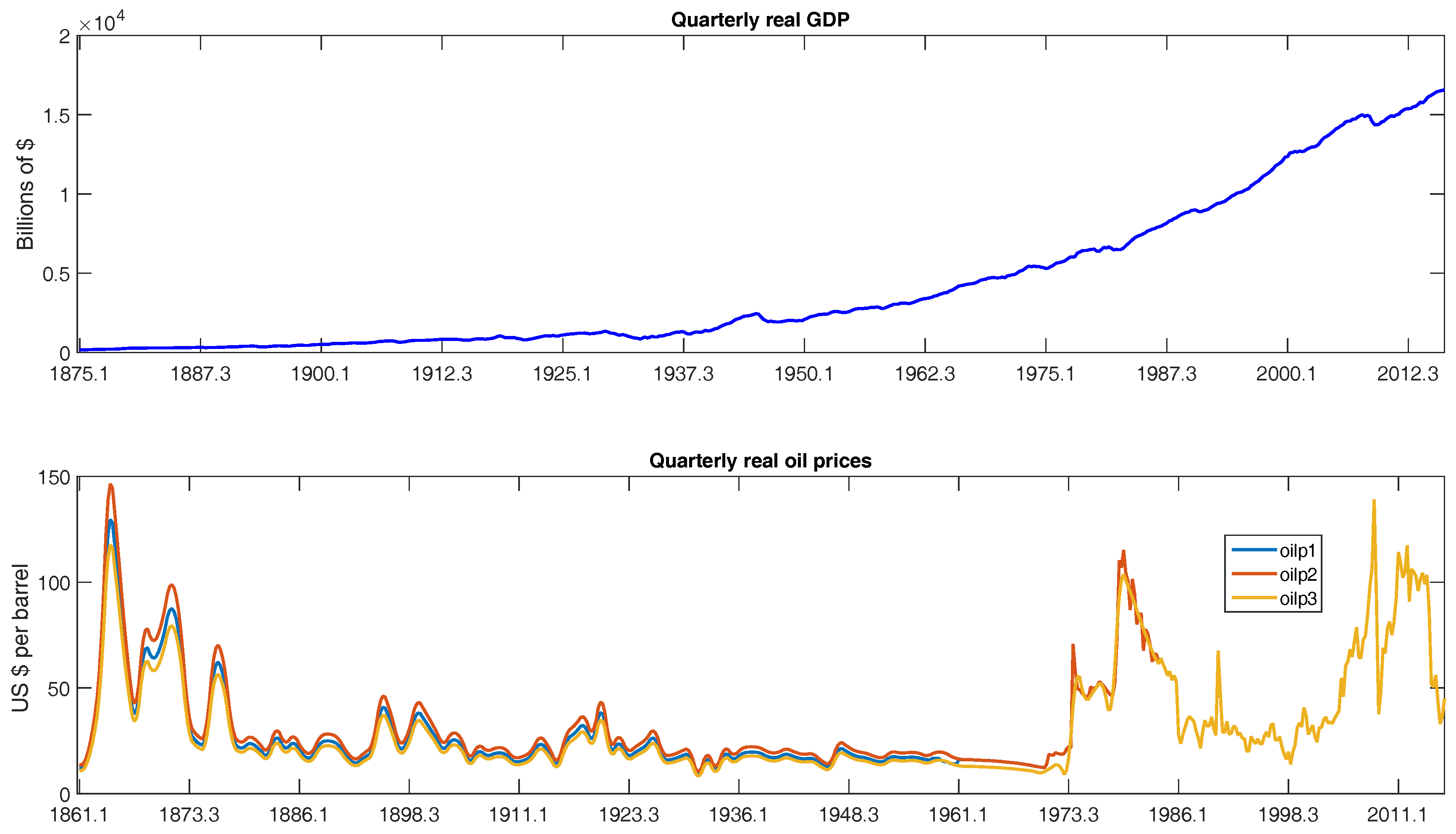
The long crude oil price series in real terms is taken from the British Petroleum’s Statistical Review of World Energy [11]. This series has an annual frequency and links three different price series: US average price (1861–1944), Arabian Light (1945–1983), and Brent (1984–2015). Since our aim is to analyze the relationship between oil price shocks and GDP, we adopt two strategies to be able to work with higher-frequency data, which would allow us to better capture the effects of oil prices on economic growth. First, we use the Chow-Lin interpolation technique [12] to convert the annual series of oil prices into a quarterly series dataset, using an intercept as high frequency indicator.4 Figure 1 displays both historical series. Second, in the last part of our sample, we work with real quarterly Brent data from Datastream.5 We have considered three options to link this quarterly series with the transformed annual data: (i) begin using the quarterly series in 1957, the first year for which Brent data are available; (ii) delay the use of the quarterly series until the 1970s, when data variability clearly increases; (iii) maintain the first two consecutive series of the British Petroleum database and link with the quarterly series in 1984. Figure 2 illustrates the different options, and we observe hardly any difference among the three (called oilp1, oilp2, and oilp3, respectively). To obtain more reliable quarterly data, we chose the Brent quarterly series beginning in 1957 (oilp3).6 This series is more accurate due to its higher frequency and is directly obtained from Datastream. Thus, our final crude oil price time series consists of the quarterly interpolated British Petroleum historical dataset until 1956, linked to the quarterly Brent data from 1957 onward, and ranges from January 1861 to February 2016. Figure 3 displays the growth rates of oil prices and GDP, calculated as the first logarithmic differences, which we denote as and , respectively.
3. Univariate Analysis of the Series
In this section, as a first data exploratory analysis, we examine the univariate evolution of each of the two series, oil prices and GDP growth rates. In particular, we explore the possible existence of structural changes in both mean and variance of the series.
3.1. Changes in Mean
In this subsection, we test for the presence of structural breaks in the mean of ΔGDP and ΔOILP. To this end, we apply the methodology of Bai and Perron [15,16,17] (BP, henceforth).7 The BP methodology looks for multiple structural breaks, consistently determining the number of break points over all possible partitions, as well as their location, and it is based on the principle of global minimizers of the sum of squared residuals. The methodology considers m possible breaks ( regimes) in a general linear model of the type:
where the explanatory variables β and are the corresponding vectors of the coefficients and are the break points, which are treated endogenously in the model.
Using this method, [15] proposes three types of tests. The first one, called the test, considers the null hypothesis of no breaks against the alternative of k breaks. The second test, , considers the existence of l breaks, with , as , against the alternative of changes. Finally, the so-called double maximum tests and (the third type) test the null of the absence of structural breaks against the existence of an unknown number of breaks. The strategy suggested by Bai and Perron [16] consists of first beginning with the sequential test . In case no break is detected, they recommend checking this result with the and tests to determine whether at least one break exists. When this is the case, they recommend continuing with the sequential application of the test, with In addition, information criteria such as the traditional Schwarz Bayesian information criterion (SBIC) and the modified Liu Wu Zidek criterion (LWZ)8 are used to select the number of changing points.
This strategy has been followed to explore the existence of structural breaks in a model representing the mean of the variables, that is, a model with just a constant: and . The disturbance term is allowed to present both autocorrelation and heteroskedasticity. A maximum number of five breaks has been considered in accordance with a sample size of for GDP growth and 621 for oil price growth. Then, according to the length of the series, the selected trimming is . A non-parametric correction has been employed to consider these effects. Table 1 shows the results. According to the different tests, we cannot reject the hypothesis that neither ΔGDP nor ΔOILP presents structural changes in the mean.9 For the whole period, the mean GDP growth is 0.80% and the mean oil price growth, 0.19%.
3.2. Changes in Volatility
To test for the possibility of structural breaks in the variance of the process, we consider the Inclán and Tiao (IT) test [21]. This test, which has been extensively used, allows for the detection of changes in the unconditional variance of a series and belongs to the CUSUM-type family of tests. The test is defined as follows:
This test assumes that the disturbance in equation , being or , is a zero-mean, normally i.i.d. random variable and uses an iterated cumulative sum of squares () procedure to detect the number of breaks. However, [22] shows that the asymptotic distribution of the IT test is critically dependent on normality. Indeed, the IT test has large size distortions when the Gaussian innovation assumption is not met in the fourth-order moment, or for heteroskedastic conditional variance processes, and consequently tends to overestimate the number of breaks.10 To overcome this drawback, they propose a correction that explicitly takes into account both the fourth-order moment properties of the disturbances and the conditional heteroskedasticity ( and , respectively).
where is a consistent estimator of
The US GDP growth series is not mesokurtic (in fact, its excess kurtosis series is 3.15) and has a fat right tail. Moreover, the conditional variance of the innovations is not constant over time.11 These properties are even more accentuated for oil price growth series, in which excess kurtosis reaches 20.10 and shows very long tails. Consequently, we use the previous corrections in addition to the original ICSS algorithm.
Table 2 shows the results of the , , and tests applied to the US GDP and oil price growth rates. We observe overestimation of break dates when using the original IT test (and even in the test), which is especially dramatic for oil price growth, considering the properties of this series. Therefore, we focus on the results of the test, which includes all corrections. We find three breaks in the variance of GDP growth, chronologically located in April 1917, February 1946, and January 1984, confirming the findings of [19].12 These break dates approximately match the end of each of the world wars and the beginning of the Great Moderation. Thus, a secular reduction in volatility is observed in US GDP growth.
The results of the variance tests applied to the oil price growth rate show only two changes in variance, in April 1878 and April 1973. Indeed, oil prices are more volatile in the beginning and ending periods (the last period being significantly more volatile), while a much less volatile period is observed from 1878 to 1973 (see Figure 3). These break points to are related to a combination of technological and geographic factors affecting the oil market by [7],13 along with a booming demand for oil, driven by the large-scale industrialization of the US and East Asia.14
To provide robustness to the previous results, we use an additional test within the parametric framework, which consists in applying the BP test to the mean of the absolute value of the estimated residuals from one of the following specifications:15
where represents or .
Table 3 roughly confirms the test results. We focus on the results of Model 1. Regarding the identification of structural breaks in the GDP growth rate, we identify three break points as in the previous exercise. However, the dates differ, as a structural break in March 1929 coincides with the 1929 Crash as against the one related to the end of the first world war.16 Concerning the oil prices, we find three break points instead of two. The new break point is located in February 1935, while the other two are the same previously identified. This methodology to the annual series of oil prices by [7], finding roughly the same three break points. They link the new break to both a major oil discovery a few years earlier (the East Texas oil Field) and a worldwide recession.
4. Multivariate Analysis of the Series
After studying the univariate evolution of both oil price and GDP growth rates, this section analyzes the transmission of the effects between them and their direction. To this end, we first use a standard VAR methodology and, subsequently, consider different methodologies to take into account the possible instability of the VAR parameters. In particular, we compute a rolling causality test and cumulative impulse response functions. In addition, we analyze the presence of structural breaks in our VAR equation.
4.1. VAR Estimation
A simple way to analyze the dynamic relationship between oil price variations and GDP growth is the use of a standard VAR(p) model. Following [30,31], among many others, we define this model as follows:
where is a 2 × 1 vector composed of observations of the variables, are 2 × 2 coefficient matrices, with is an unobservable zero mean white noise vector of dimension T, and p is the parameter that determines the VAR dimension, chosen according to the SBIC criterion.17 The model is specified as follows:
The VAR estimation is reported in Table 4. The results show no significant effect of oil price growth on GDP growth, which means does not influence—that is, does not Granger-cause—GDP growth. We obtain a similar result in the opposite direction, as the effect of GDP growth on oil price growth is not significant.
Furthermore, the parameter is negative and is positive. This means that the effect of oil price growth on output growth is negative, while the effect of GDP growth on oil price is positive. Although these findings are quite suggestive and support our intuition about the causal effects between GDP and oil prices, we test them more formally.
The previous framework allows us to test for causality direction. Following [32], a variable (or group of variables), , is found to help predict another variable (or group of variables), . Then, is said to Granger-cause . We can test this hypothesis by simply studying whether the Ψ matrices are triangular, which is a remarkably visual test for a VAR(1). Additionally, a more formal Wald test is computed, where the null hypothesis is that does not cause . More specifically, does not lead to if .18 The results of the Granger causality analysis are presented in the last rows of Table 4, confirming the previous findings.19
We also employ impulse-response functions (IRFs) to capture the dynamics of the shocks. To obtain IRFs, we use a moving average representation of the VAR system, which is defined in the following expression:
or in matrix notation and in terms of the innovations of the structural model: .
The coefficients of the succession of matrices represent the impact that a shock in the structural innovation has on the variables of the VAR system over time. Results of IRF computations with a horizon of 5 years (20 quarters) are displayed in Figure 4, where confidence intervals at 90% are computed according to bootstrap-after-bootstrap method of [33]. We conclude that the effects, which are negative for the response of to an impulse of and positive for the response of to an impulse of , last between 7 and 8 quarters and are not significant at any length. We also observe a high degree of uncertainty during the time of non-zero IRFs.20
In addition, we compute cumulative impulse-response functions (CIR), defined as , which allow us to identify the same effects in the long run. Thus, considering the full period (February 1875–February 2016), has a negative effect (−0.0057) on , while has a positive effect (0.3306) on , although neither is significant.21
Summing up, we do not observe any significant effect between changes in oil prices and GDP growth when considering the full period. Nevertheless, it is reasonable to think that in such a long period in which significant events have occurred, both in the business cycle dynamics and in the demand and supply factors of oil prices, the relationship between the two variables may have not been so stable. In fact, our findings in the previous section already show several structural breaks in volatility that correspond to important changes in the characteristics of the business cycle and different periods in the evolution of oil prices. The hypothesis of a changing relationship is explored in the following subsections.
4.2. Rolling Sample Analysis
The previous section provides some insights about the direction of the relationship between oil inflation and the US GDP growth. However, it is possible that this relationship has been modified across time, as suggested by [4]. Thus, it is advisable to estimate the model for different subsamples in order to verify whether the parameters change. In this regard, we adopt two alternative strategies: (i) compute causality test and (ii) calculate CIRs, as a measure of long-run impacts, instead of using short-run parameters. We consider a rolling estimation with a window of 40 quarters in both cases.
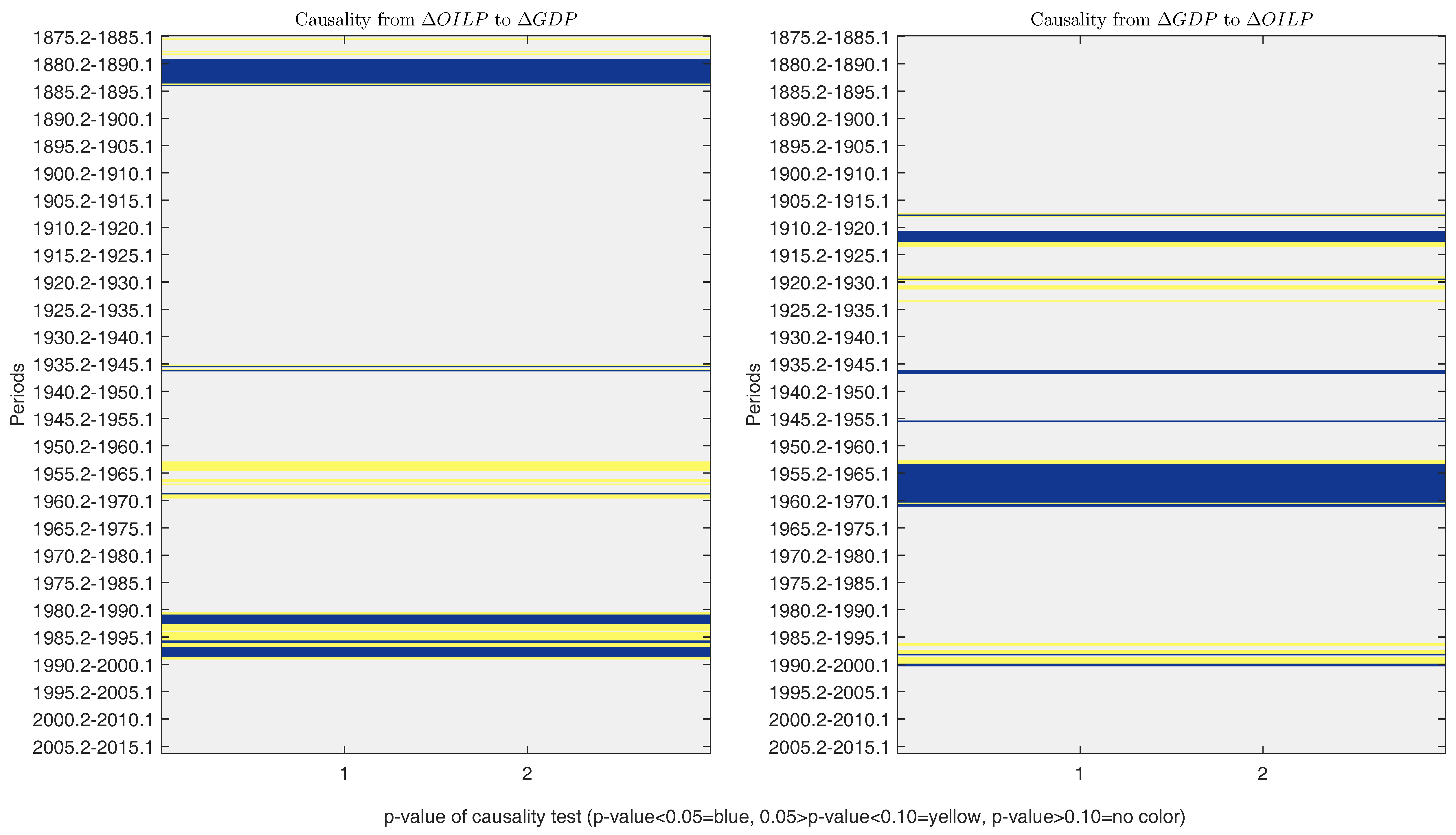
Regarding the causality test, results are displayed in Figure 5, which plots a heat map of p-values of the Granger causality test. Different colors represent the different significance levels at which we can reject or accept the Granger causality test. Values in yellow and dark blue mean that we can reject the null hypothesis of non-causality, whereas values in no colour indicate no causality between the variables. In general, we scarcely observe periods of significant causality, given the overwhelming presence of no color in the figure. Focusing on causality from to (left-hand side of the figure) and with a liberal threshold of the 0.10 significance level, we identify two stable and long periods where oil prices clearly influence GDP growth: January 1879–April 1894 and January 1981–February 1999. In the rest of the period, we only find isolated dates during mid-20th century (the 1950s) and at the beginning of the period, before April 1879. Results basically hold when considering a tighter significance level of 5%, although the instability during the 1980s and 1990s increases. To sum up, the influence of oil price growth on GDP growth is significant only for 14% of the sample at the 10% significance level.
As for the opposite direction of causality, from to (right-hand side of the figure), the proportion of the sample where the influence is significant is similar at 10% level but reduces to 9% at the 5% significance level. Periods of causality from GDP growth to oil price variations are found in February 1911–April 1923, February 1953–February 1971, and February 1988–February 2000.22 We conclude that the relationship between the two variables is relatively weak in the long run. However, at shorter horizons, the major intensity in the bidirectional relationship is located in the 1980s and 1990s.
With respect to CIRs, Figure 6 displays the results of impulses from to (upper panel) and from to (lower panel). Focusing on the rolling estimation of CIRs between the two variables, we observe that the estimated response to an impulse from to remains close to zero, and non-significant, over the whole sample, except for the estimated impulse response over the periods 1961–197123 and 1937–1946.24 The estimated impulse from to presents higher variability. Indeed, from the mid-1960s to the end of the century, it is positive most of the time. The effect turns negative during the noughties of the 21st century. Nonetheless, the confidence intervals show no significant effect in the short periods, also identified in the upper panel of the figure.25
4.3. Structural Breaks in the Relationship between Oil Prices and GDP
The univariate analysis of the series offers some evidence of structural breaks in the volatility of the two series. Additionally, the rolling results of the previous subsection are not conclusive about the hypothesis of parameter stability. Thus, it seems to be appropriate to consider the existence of structural breaks in our multivariate specification. To that end, the Qu and Perron (QP) [9] approach provides a valid technique to find structural breaks,26 as it allows for multiple structural changes that occur at unknown dates in a general system of equations, which indeed include the one defined in (10).
Following these authors, we assume that we have n equations and T observations, the vector includes our two endogenous variables ( and ), the parameter q is the number of regressors, and is a set that includes the regressors from all the equations. The selection matrix S is of dimension with full column rank, where q is the total number of parameters. It involves elements that take the values 0 and 1, indicating which regressors appear in each equation. The total number of structural changes in the system is m, and the break dates are denoted by the m vector , considering that and , with j indexing the regime . Then, the model proposed takes the following form:
with having mean 0 and covariance matrix for . In our present case, we should note that , and , where and p is the selected number of lags. Again, the number of lags has been chosen by taking into account the SBIC.
To determine the number of breaks in the system, we first use the statistics to test whether at least one break is present. When the tests reject it, the test is sequentially applied for until it fails to reject the null hypothesis of no additional structural break. Additionally, we compute the to test versus .
According to the critical values derived from the response surface regressions, the tests offer evidence of three breaks () in the system of equations, which satisfies the minimal length requirement, notice that because of our sample size (), we have carried out the procedure with a trimming parameter of 0.2. Results of the application of this procedure are reported in Table 5. The three break dates are located in April 1912, January 1941, and March 1970. Notice that the first two breaks are quite close to those identified in the univariate analysis of structural breaks in volatility of the GDP growth, while the third break is near the last structural volatility break in oil prices. Hence, we identify four different periods in the relationship between oil price shocks and the US GDP growth.27 For each of the four periods, we repeat the analysis presented in Section 4.1. The number of lags for each period has been selected according to different information criteria (they appear in brackets in Table 5).
The first interval covers the period between January 1875 and April 1912. Thus, the imminent beginning of World War I (WWI, henceforth) marks the end of this period. The sample begins just after the panic of 1873, when the US was still facing its economic consequences. A few years later, the US economy had to cope with the aftermath of the 1893 panic, while already in the 20th century, the US economy faced WWI (1914–1918). Regarding oil prices, this period is characterized by the evolution of the oil industry along with the exhaustion in production of key oil fields, at a time in which the demand was strong.
The second period starts in January 1913 and ends in the early 1940s. During that time, the US economy was affected by some of the most influential economic events of the 20th century, such as the Crash of 1929, with devastating economic effects during the next decade, and WWII (1939–1945). Concerning the historical oil price shocks, this period was much influenced by the Great Depression, with an associated decline in oil demand, and the introduction of state regulation of industry and restrictions on competition. No Granger causality is identified from any of the two variables to the other in either of the first two subperiods.
The third period runs from February 1941 to March 1970. In terms of the US economy dynamics, this period is characterized by a post-war economic boom that lasted until the 1970s. Indeed, during the 1950s, and especially the 1960s, the US experienced its longest, almost uninterrupted period of economic expansion in history. Oil prices were quite stable during this period. OPEC was established in 1960 with five founding members. Throughout the post-WWII period, exporting countries experienced an increasing demand for oil, and the volume of oil that Texas producers could produce was no longer limited, but the power to control crude oil prices shifted from the US to OPEC. During this period of economic boom, has a significant effect on .
Finally, the last period begins in the early 1970s and ends in February 2016. The 1970s were characterized by the end of the Bretton Woods system and substantial oil price shocks, economic growth became stagnant, and inflation grew. In the 1980s, these disequilibria were reversed, and the US economy witnessed a reduction in the volatility of the business cycle. The last period of the sample (from 1984 on) is called the Great Moderation. During this period, the US enjoyed long economic expansions, interrupted only by three recessions, the last one being the Great Recession (2007–2009), which was followed by a weak recovery. The evolution of oil prices during this period and its effect on macroeconomic performance have been extensively studied in the literature. The US, as did most industrialized economies, became heavily dependent on imported crude oil from the Middle East, and the 1970s were a tumultuous decade in terms of oil market events.28 Other political events that influenced oil prices took place during the rest of the period.29 During this final period, the effect of on is significant at 10%.
To sum up, the Granger causality between the two variables is significant only in two periods. has a significant effect on , on the one hand, in the February 1941–March 1970 sample, when the US economy experienced a huge economic boom, and, on the other, in the March 1970–February 2016 sample (in the opposite causality direction), when oil price shocks exerted a significant influence on economic performance.
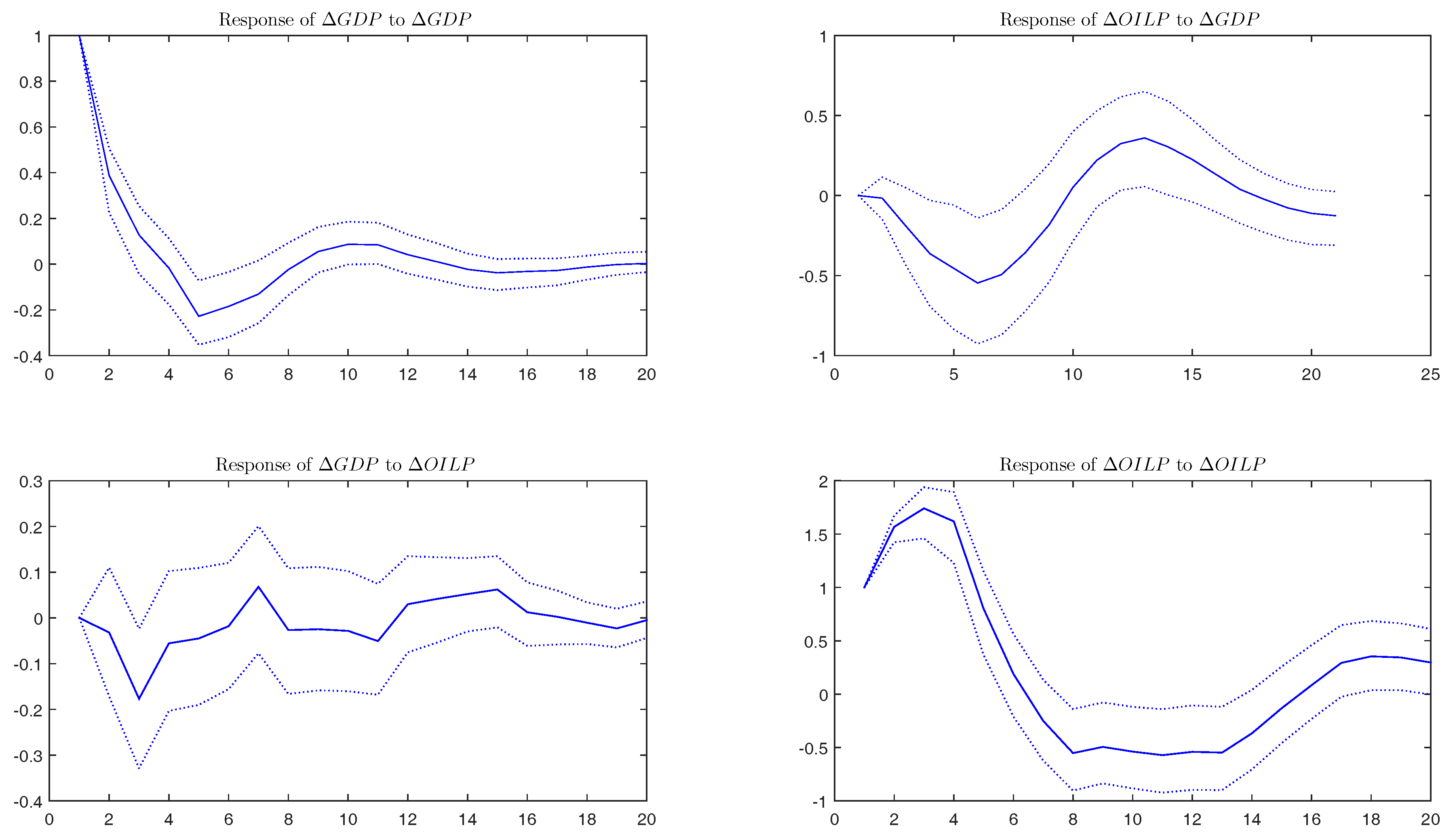
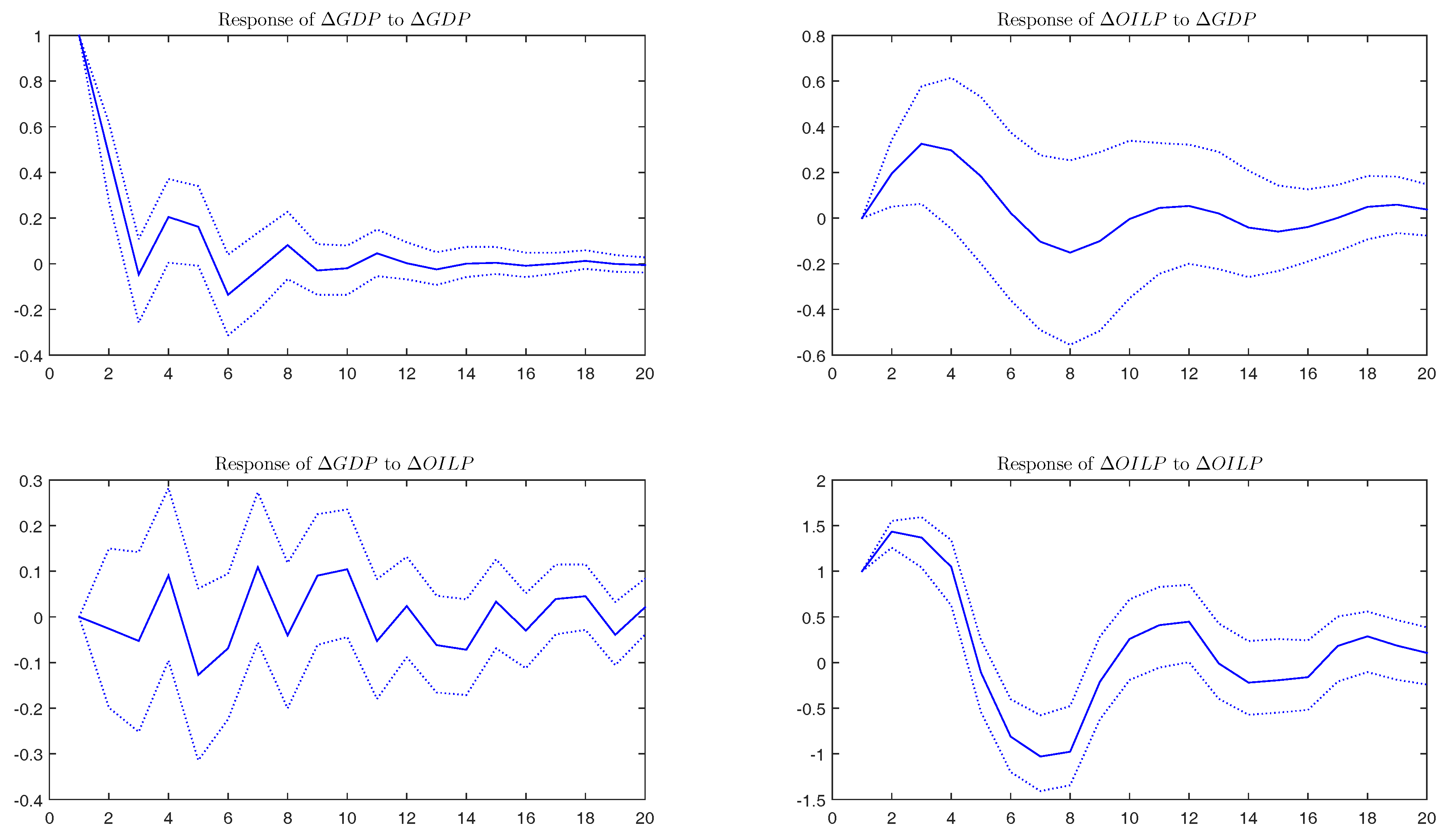
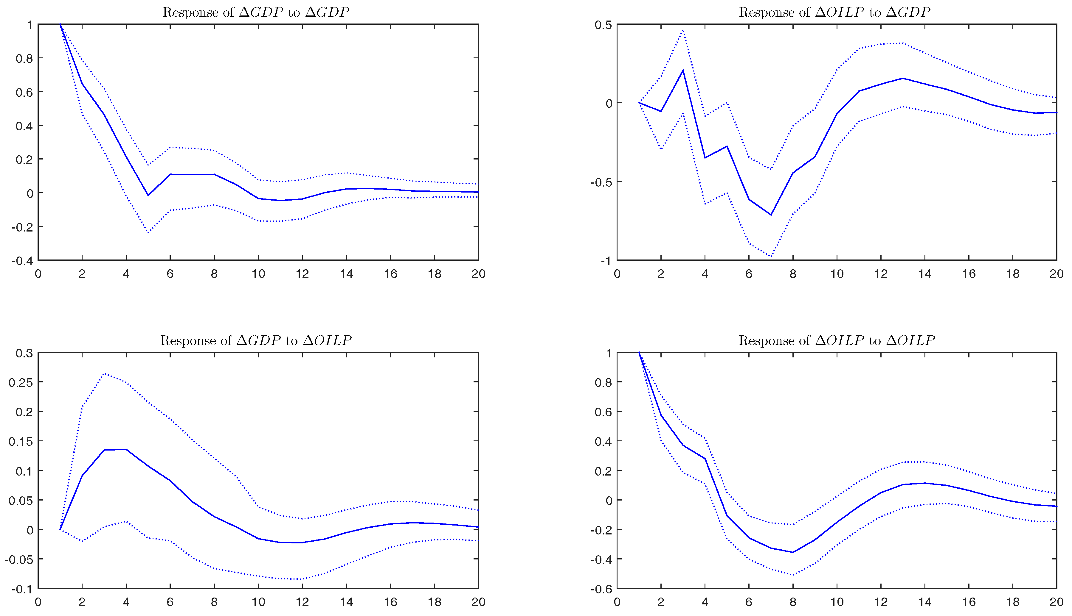
Figure 7, Figure 8, Figure 9 and Figure 10 display IRFs in different regimes delimited by structural breaks. We observe that has a negative effect on in all periods except February 1941–March 1970. Regarding the effect of the shock on , the sign changes, highlighting the positive influence in the last period. Nevertheless, these effect are non significant for the most part of all sub-periods.
5. A Time-Varying GDP-Oil Price Model
In previous sections, we find ample evidence of instability and non-linearities in the relationship between real GDP growth and oil price shocks. In this section, we use a more subtle and sophisticated econometric tool, a time-varying structural VAR model, to further explore the relationship between the two variables. Following [35], we consider the model
where is a 2 × 1 vector of time-varying coefficients for the constant term; is a 2 × 2 matrix of time-varying coefficients, and contains heteroskedastic unobservable shocks with the variance-covariance matrix . After a triangular reduction of , we obtain the following model:
where is a lower triangular matrix and is a diagonal matrix.
The time-variant nature of the VAR model derives both from the coefficients and the variance-covariance matrix of the innovations. Its estimation is based on a Markov chain Monte Carlo algorithm with a Bayesian approach.30
The identification conditions of the model allow us to capture oil price shocks affecting GDP growth, but these shocks are exogenous to GDP growth, as well as the reaction of oil prices to GDP growth evolution. Thus, we focus on exogenous oil price shocks, which can be isolated in the time-varying system and are more relevant considering the previous analysis. Figure 11 presents the posterior mean of the time-varying standard deviation of oil price shocks. The post-1970s period exhibits a substantially higher variance of oil price shocks than other periods. Although not our primary concern, the time-varying standard deviation of GDP growth, too, reveals interesting results. We can observe a secular decline in volatility and identify several periods delimited by WWII and the Great Moderation.31
More interestingly, the time-varying VAR approach allows us to calculate IRFs at different points of time and assess different responses. The dates are not arbitrary, but capture major shocks behind the largest movements in oil price markets, which could have exerted an influence on the economic conditions regarding the relationship between oil prices and GDP growth in those dates. In particular, we select the oil price downturns of April 2014, April 2008, January 1986, January 1991, and March 2008, ordered from the highest to the lowest decline (−91.1%, −65.1%, −51.4%, −48.0%, and −39.6%, respectively), and the increases that took place in January 1974, March 1990, February 1979, February 2009, and January 1999, from the highest to the lowest value (118.2%, 89.5%, 41.5%, 36.6%, and 35.1%, respectively). They are displayed in Figure 12. In the following paragraphs, we describe the events affecting world oil markets during these dates in chronological order.
The Arab oil-exporting nations’ embargo of 1973 against countries (in particular, the US and many other developed countries) supporting Israel in the Yom Kippur War, at a time of rising demand and decreasing OPEC production, caused oil prices to abruptly increase. Specifically, by the first quarter of 1974, the increase reached 118.2%.
From 1974 to 1978, crude oil prices were relatively flat, but the crises in Iran and Iraq in 1979 and 1980 led to a new round of increases. Indeed, the Iranian revolution was the cause of one of the highest oil price rises, in spite of its relatively short duration. In the second quarter of 1979, the oil price jump was 41.5%.
In 1986, there was a collapse in crude oil prices, which was due to the fact that the OPEC cut output significantly to defend its official price in response to declining world oil demand and increasing production in non-OPEC countries. In the first quarter of the year, the decrease in oil prices reached 65.1%.
The Persian Gulf War also affected world oil markets. The Iraqi invasion of Kuwait in 1990 caused a rapid oil price escalation. Indeed, in the third quarter of 1990, oil prices rose by 89.5%. However, after two months of oil price increases, the United Nations approved the use of force against Iraq and oil prices began falling. In the first quarter of 1991, oil prices diminished by 48%.
In early 1999, oil prices began to grow, after the downward trend during the previous year, caused by a decline in consumption in Asian economies and higher OPEC production. This rise in oil prices was due to the reduction of OPEC production. This organization decided to cut production by about three million barrels per day, and the increase in oil prices in the first quarter of 1999 was 35.1%.
In 2008, after the Great Recession began,32 falling petroleum demand, at a time when speculation in the crude oil futures market was exceptionally strong, decreased oil prices. In the third quarter of 2008, this decrease was 39.6%, while in the fourth quarter, the decline deepened to 91.1%. Nevertheless, an OPEC production cut in early 2009, some tensions in the Gaza Strip, and a rising demand from Asian countries increased oil prices steadily. In the second quarter of 2009, oil prices peaked at 36.6%.
The oil price decline in 2014 came after a period of stability. This drop was due to several factors. There was a slowdown in global economic activity. Indeed, the same countries that pushed up the price of oil in 2008 helped bring oil prices down in 2014. The US and Canada increased their production of oil, cutting their oil imports sharply, which put further downward pressure on world prices. Furthermore, Saudi Arabia decided to keep its production stable in order not to sacrifice their market share and restore the price. The oil price decline in the fourth quarter of 2014 was −91.1%.33
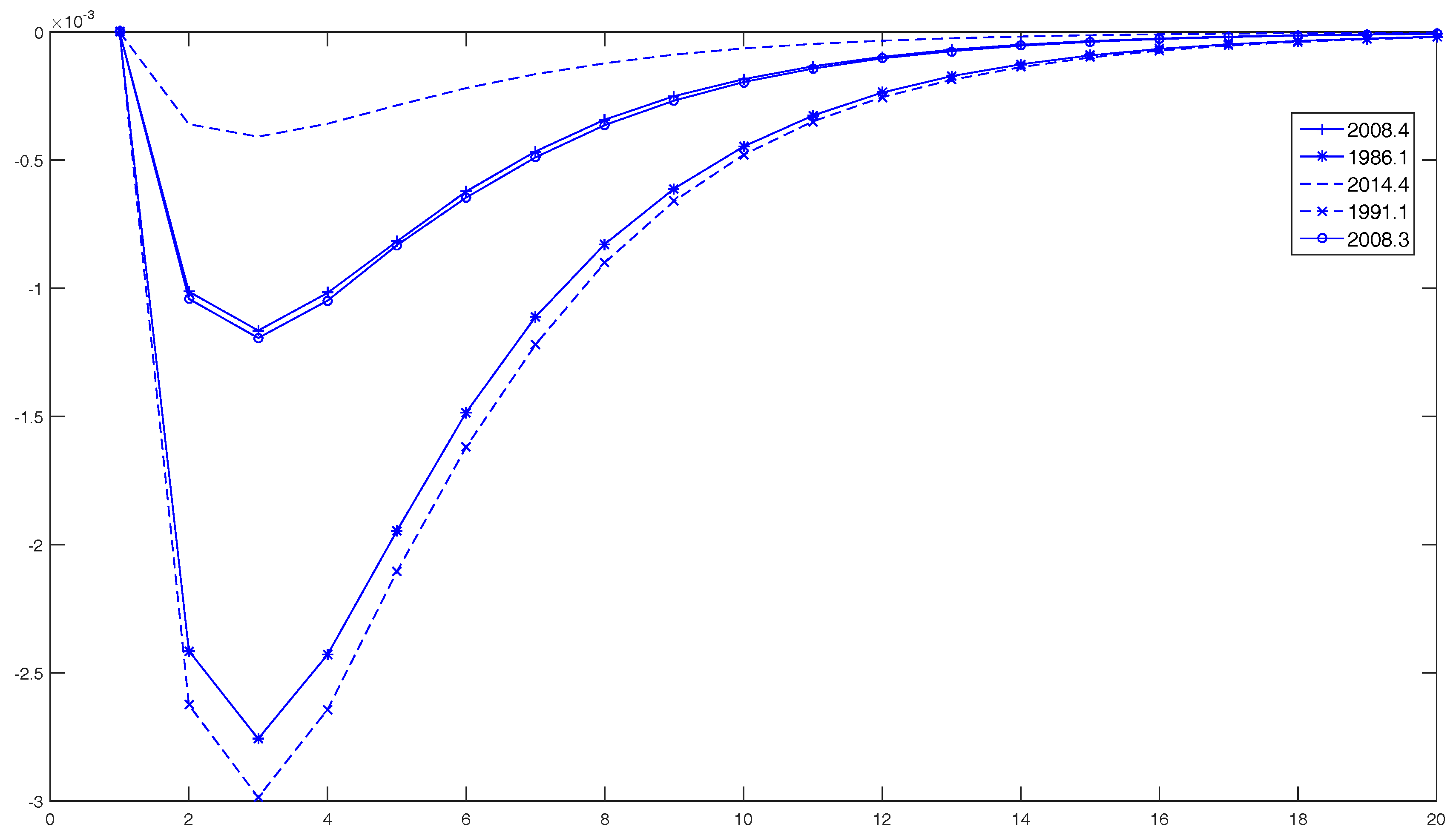
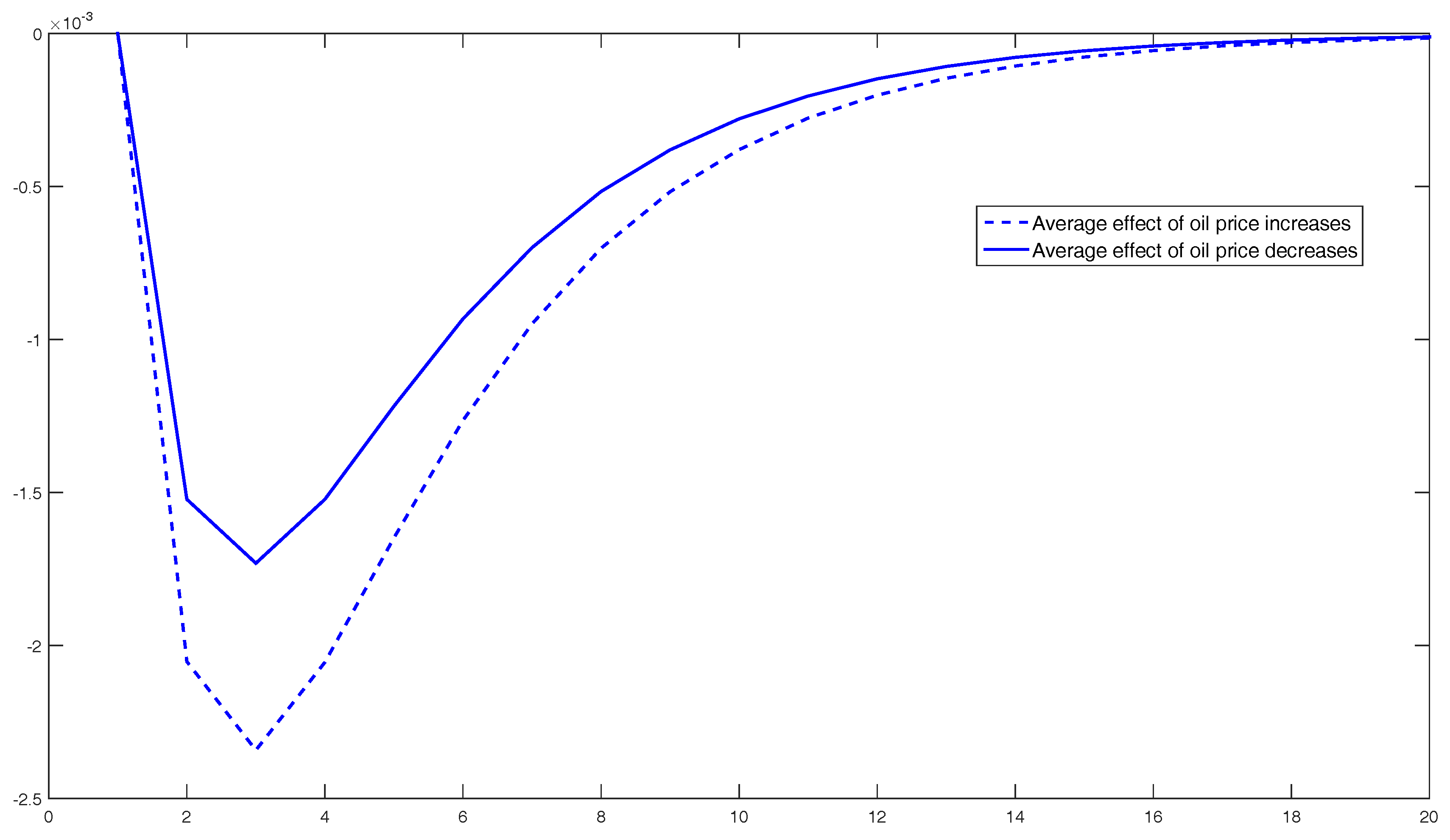
Results of impulse-response analysis over time are displayed in Figure 13 and Figure 14. It should be noted that at selected dates (either increases or decreases), we introduce a normalized shock in the model (always positive) to see to what extent the conditions of the economy could have changed over time. Oil price growth shocks have temporary effects on GDP growth. At the time of large oil price increases, we observe a GDP decline over the first three quarters, while at the time of large oil price decreases, the effect on GDP is not so clear. However, confidence intervals are quite large during the first two years and a half. Figure 15 and Figure 16 compare the magnitude of GDP growth changes in different periods. We observe that all the oil price increase dates considered have a similar negative effect on GDP growth, except the one in February 2009. We find the same pattern for the effect of oil price decreases. The impact of an oil price shock on GDP growth has declined over time, although there is more dispersion among different episodes in this case. Overall, oil price elasticity with respect to GDP has declined.34 Finally, Figure 17 compares the average effects at the time of large oil price increases and decreases. We observe that the negative effect of oil price shocks on GDP growth is greater at the time of large oil price increases, which confirms previous evidence of nonlinearity in the relationship [37].
6. Conclusions
This study analyzes the relationship between oil prices and GDP from a long-term perspective, from the last third of the 19th century, when crude oil started to be commercially produced in Pennsylvania, to the present. Using different econometric tools, we analyze the individual dynamics of the series, as well as their interaction. The univariate study of the series shows that none of them presents structural breaks in mean. However, this apparent tranquility hides a considerable, and divergent, volatility. While real GDP growth has evolved into a secular volatility reduction, the variability of oil prices has substantially changed over the sample period.
Considering the whole sample, the evidence of the influence between GDP and oil prices is extremely weak, and not statistically significant, which could be due to the fact that there are instabilities in the relationship masking it. Indeed, over such a long period there have been important changes in the demand and supply for oil that could lead to identify some structural breaks. Therefore, we use several econometric techniques to detect and isolate different episodes, finding three break dates which are located in 1912, 1941, and 1970. Only this last period has been thoroughly studied in the literature.
We find that the period of the strongest relationship, characterized by a negative effect of oil price increases on GDP growth, occurs after the 1970s. However, in this last period, a time-varying model shows a decline in the impact of oil price shocks on GDP growth since then. Furthermore, we identify an asymmetric effect between large oil price increases and decreases. We notice that the negative effect of oil price shocks on GDP growth is greater at the time of large oil price increases. We also observe that the response of GDP to oil is significant over the periods 1961–1971 and 1937–1946.
Overall, the story of the relationship between GDP and oil prices is relatively turbulent. Although our findings point to a negative influence from oil price increases on economic growth, this phenomenon is far from being stable and has gone through different phases over time. Further research is necessary to fathom this complex relationship.
Acknowledgments
The authors acknowledge financial support of the Ministerio de Ciencia y Tecnología under grants ECO2014-58991-C3-1-R and ECO2014-58991-C3-2-R (M. Dolores Gadea) and ECO2015-65967-R (A. Montañes). The views expressed in this paper are the responsibility of the authors and do not necessarily represent those of the Banco de España or the Eurosystem.
Author Contributions
The authors contributed equally to this work.
Conflicts of Interest
The authors declare no conflict of interest.
References
- J.D. Hamilton. “Oil and the macroeconomy.” In The New Palgrave Dictionary of Economics. Edited by S.N. Durlauf and L.E. Blume. London, UK: Palgrave Macmillan, 2008. [Google Scholar]
- L. Kilian. “The Economic Effects of Energy Price Shocks.” J. Econ. Lit. 46 (2008): 871–909. [Google Scholar] [CrossRef]
- O.J. Blanchard, and J. Galí. The Macroeconomic Effects of Oil Price Shocks: Why are the 2000s so different from the 1970s? In International Dimensions of Monetary Policy. NBER Chapters; Cambridge, MA, USA: National Bureau of Economic Research, Inc., 2007, pp. 373–421. [Google Scholar]
- A. Gomez-Loscos, M.D. Gadea, and A. Montañés. “Economic growth, inflation and oil shocks: Are the 1970s coming back? ” Appl. Econ. 44 (2012): 4575–4589. [Google Scholar] [CrossRef]
- J.D. Hamilton. “Oil and the Macroeconomy since World War II.” J. Political Econ. 91 (1983): 228–248. [Google Scholar] [CrossRef]
- A. Gómez-Loscos, A. Montañés, and M.D. Gadea. “The impact of oil shocks on the Spanish economy.” Energy Econ. 33 (2011): 1070–1081. [Google Scholar] [CrossRef]
- E. Dvir, and K.S. Rogoff. Three Epochs of Oil. NBER Working Paper; Cambridge, MA, USA: National Bureau of Economic Research, Inc., 2009. [Google Scholar]
- K. Mohaddes, and M.H. Pesaran. “Oil prices and the global economy: Is it different this time around? ” USC-INET Reseach Paper, No. 16-21. 2016. Available online: https://papers.ssrn.com/sol3/papers.cfm?abstract_id=2808084 (accessed on 6 June 2016).
- Z. Qu, and P. Perron. “Estimating and testing structural changes in multivariate regressions.” Econometrica 75 (2007): 459–502. [Google Scholar] [CrossRef]
- R.J. Gordon. The American Business Cycle: Continuity and Change. NBER Book Series Studies in Business Cycles; Cambridge, MA, USA: National Bureau of Economic Research, 1986. [Google Scholar]
- British Petroleum. BP Statististical Review of World Energy. Technical report; London, UK: British Petroleum, 2016. [Google Scholar]
- C. Chow, and A.L. Lin. “Best linear unbiased interpolation, distribution, and extrapolation of time series by related series.” Rev. Econ. Stat. 53 (1971): 372–375. [Google Scholar] [CrossRef]
- J. LeSage. “Applied Econometrics Using MATLAB.” 1999. Available online: http://www.spatial-econometrics.com/html/mbook.pdf (accessed on 9 July 2016).
- E.M. Quilis. “A Matlab library of temporal disaggregation methods.” Instituto Nacional de Estadística, Internal Document, Madrid, Spain, 2004. [Google Scholar]
- J. Bai, and P. Perron. “Estimating and Testing Linear Models with Multiple Structural Changes.” Econometrica 66 (1998): 47–78. [Google Scholar] [CrossRef]
- J. Bai, and P. Perron. “Computation and analysis of multiple structural change models.” J. Appl. Econom. 18 (2003): 1–22. [Google Scholar] [CrossRef]
- J. Bai, and P. Perron. “Critical values for multiple structural change tests.” Econom. J. 6 (2003): 72–78. [Google Scholar] [CrossRef]
- J. Liu, S. Wu, and J. V. Zidek. “On Segmented Multivariate Regressions.” Statistica Sinica 7 (1997): 497–525. [Google Scholar]
- M.D. Gadea-Rivas, A. Gómez-Loscos, and G. Pérez-Quirós. The Great Moderation in Historical Perspective. Is It That Great? CEPR Discussion Paper No. 10825; London, UK: Center for Economic Policy Research, 2014. [Google Scholar]
- D.W.K. Andrews. “Heteroskedasticity and Autocorrelation Consistent Covariance Matrix Estimation.” Econometrica 59 (1991): 817–858. [Google Scholar] [CrossRef]
- C. Inclán, and G.C. Tiao. “Use of Cumulative Sums of Squares for Retrospective Detection of Changes of Variance.” J. Am. Stat. Assoc. 89 (1994): 913–923. [Google Scholar] [CrossRef]
- A. Sanso, V. Arago, and J.L. Carrion-i Silvestre. “Testing for changes in the unconditional variance of financial time series.” Revista de Economia Financiera 4 (2004): 32–53. [Google Scholar]
- A. Deng, and P. Perron. “The Limit Distribution of the Cusum of Squares Test Under General Mixing Conditions.” Econom. Theory 24 (2008): 809–822. [Google Scholar] [CrossRef]
- J. Zhou, and P. Perron. Testing for Breaks in Coefficients and Error Variance: Simulations and Applications. Working Papers Series No. wp2008-010; Boston, MA, USA: Department of Economics, Boston University, 2008. [Google Scholar]
- G. Fagiolo, M. Napoletano, and A. Roventini. “Are output growth-rate distributions fat-tailed? some evidence from OECD countries.” J. Appl. Econom. 23 (2008): 639–669. [Google Scholar] [CrossRef]
- J.D. Hamilton. Historical Oil Shocks. NBER Working Paper No. 16790; Cambridge, MA, USA: National Bureau of Economic Research, Inc., 2011. [Google Scholar]
- A.M. Herrera, and E. Pesavento. “The Decline in U.S. Output Volatility: Structural Changes and Inventory Investment.” J. Bus. Econ. Stat. 23 (2005): 462–472. [Google Scholar] [CrossRef]
- J.H. Stock, and M.W. Watson. Has the Business Cycle Changed and Why? NBER Working Paper No. 9127; Cambridge, MA, USA: National Bureau of Economic Research, Inc., 2002. [Google Scholar]
- M.D. Gadea, A. Gomez-Loscos, and G. Perez-Quiros. The Two Greatest. Great Recession vs. Great Moderation. CEPR Discussion Paper Series No. 10092; London, UK: Center for Economic Policy Research, 2014. [Google Scholar]
- C. Sims. “Macroeconomics and Reality.” Econometrica 48 (1980): 1–48. [Google Scholar] [CrossRef]
- H. Lütkepohl. Introduction to Multiple Time Series Analysis. Berlin, Germany: Springer, 2005. [Google Scholar]
- C. Granger. “Investigating Causal Relations by Econometric Models and Cross Spectral Methods.” Econometrica 37 (1969): 424–438. [Google Scholar] [CrossRef]
- L. Kilian. “Small-Sample Confidence Intervals For Impulse Response Functions.” Rev. Econ. Stat. 80 (1998): 218–230. [Google Scholar] [CrossRef]
- M.D. Gadea, and A. Gomez-Loscos. “Oil price shocks and the US economy: What makes the latest oil price episode different.” Int. Econ. Lett. 3 (2014): 36–44. [Google Scholar]
- G.E. Primiceri. “Time Varying Structural Vector Autoregressions and Monetary Policy.” Rev. Econ. Stud. 72 (2005): 821–852. [Google Scholar] [CrossRef]
- C. Baumeister, and L. Kilian. “Understanding the Decline in the Price of Oil since June 2014.” J. Assoc. Environ. Resour. Econ. 3 (2016): 131–158. [Google Scholar] [CrossRef]
- J.D. Hamilton. “What is an oil shock? ” J. Econom. 113 (2003): 363–398. [Google Scholar] [CrossRef]
- 1.Since the seminal work of [5] for the US economy, a growing number of articles have analyzed the economic consequences of oil price shocks in industrialized countries. Most of the literature shows that the effect of oil price on the economy was very important during the 1970s, but has gradually disappeared since then (many studies support this view; the work in [2] provides a comprehensive review of the literature). The papers [4,6] show that this influence has revived, but with less intensity, since 2000 and, most important, is manifested on inflation.
- 2.The authors find that the real price of oil has historically tended to be both more persistent and more volatile whenever rapid industrialization in the world economy coincided with uncertainty regarding access to supply.
- 3.The first series is in real 2009 dollars, while the long historical series is in real 1972 dollars, but has been transformed to link both. The historical series is taken from Appendix B of [10].
- 4.Chow-Lin interpolation is a regression-based technique to transform low-frequency (annual, in our case) data into higher-frequency (quarterly, in our case) data. In particular, we apply the average version, which disaggregates the annual data into the means of four quarters and is the most suitable approach for price data, and select the maximum likelihood method. We use the Matlab toolbox of [13,14]. This approach gives us the best fit when compared to the available quarterly data. However, we have tested the accuracy of other disaggregation methods and the results remain broadly unchanged.
- 5.Prices are in 2009 US dollars per barrel, and the US GDP deflator data are from the IMF.
- 6.We have also considered other alternatives: (1) use the British Petroleum dataset, updating the last years with the annual Brent series and transforming the whole sample into quarterly data through the Chow-Lin procedure; (2) use the historical British Petroleum series linked to the West Texas Intermediate data or the Producer Price Index for crude petroleum (since they are available or from 1984 onward) instead of Brent prices. We have decided to disregard these options to obtain a more homogeneous dataset by using Brent prices. However, comparing the path of the alternative series to the one we use, we do not observe much difference. Furthermore, we repeated some calculations, obtaining quite similar results.
- 7.We have tested, but not rejected, the hypothesis that both series are I(0), using a battery of standard unit root tests. The stationarity of the series is a pre-condition for applying the BP method. Detailed results are available upon request.
- 8.See [18].
- 9.Alternatively, we tried a standard autoregressive model of order 1, with and , finding similar conclusions. The results are also robust to considering a higher number of maximum breaks. A paper by [19] also confirms the absence of structural breaks in the mean of US GDP series.
- 10.The IT approach is extended to more general processes by [23], showing that the correction for non-normality proposed by [22] is suitable when the test is applied to the unconditional variance of raw data. Furthermore, [24] carry out a Monte Carlo experiment that highlights the adequacy of this procedure when the mean or other coefficients in the regression do not change; otherwise, the test has important size distortions, which increase with the magnitude of change in the mean.
- 11.The US GDP growth rates can be approximated by leptokurtic densities as shown by [25]. This indicates that output growth changes tend to be quite uneven in the sense that large positive or negative changes seem to be more frequent than a Gaussian model would predict.
- 12.The authors offer a thorough analysis of the sources and features of these different volatility periods.
- 13.Construction of the first long-distance pipeline began in 1878, allowing the railroad monopoly over oil transportation to end. However, US control over excess exploitable reserves ended and OPEC dominance increased in 1969.
- 14.See also [26] for a historical survey of the oil industry with particular focus on the events related to significant oil price changes.
- 15.A paper by [24] shows that, in case changes in the mean of the series are not taken into account, the test suffers from severe size distortions. However, we have shown that our series do not have structural breaks in the mean. This method has been used in several studies: [27,28,29], among others.
- 16.Notice that these break points are the least significant ones with both approaches. Indeed, the break of March 1929 is not even identified with Model 2 of the BP methodology.
- 17.The SBIC criterion selects one lag. Nevertheless, other information criteria, such as the Akaike information criterion (AIC) and the Hannan-Quinn (HQ) criterion select five lags. Therefore, we use a VAR(1) as the preferred model and estimate, additionally, a VAR(5) to check the robustness of our results. For simplicity, and to save space, we only present the results for the VAR(1) and discuss whether some interesting results or significant differences appear with respect to the VAR(5).
- 18.We have repeated the analysis with annual data as a robustness check, finding qualitatively the same results.
- 19.An estimation of a VAR system with five lags does not change this conclusion.
- 20.As is well-known, the order of variables is relevant for IRF computation, as the Cholesky decomposition requires triangulation. To test the robustness of the results, we have redone all calculations with the system in the inverse order: and have also calculated the generalized IRF. The findings are the same, which is not surprising, given the results of casualty.
- 21.The confidence intervals are (−0.0269, 0.0151) and 0.3306 (−0.4279, 1.1086), respectively. They were computed with the same bootstrap methodology as for the IRFs.
- 22.Since 2005, the causality test is near the 10% threshold limit of significance. This result agrees with that of [34], who document a positive and significant effect of GDP growth on oil prices since the 2000s.
- 23.This was an extraordinary growth period in the US economy. The increasing demand for oil caused oil price increases.
- 24.During this period, the US economy had to face World War II with devastating economic consequences (the first postwar US recession began at the end of 1948). The demand for petroleum products caused a sharp increase in the price of oil and although the US increased oil production enormously during World War II, there were shortages in several plants.
- 25.We have repeated the analysis using annual data, reaching the same conclusions.
- 28.The Arab-Israel war in 1973, which followed the long-lasting Arab-Israeli conflict, and the Iranian revolution in 1978–1979 are a few examples.
- 29.Such as the Iran-Iraq war of 1980–1988, the Persian Gulf War of 1990–1991, the Venezuelan crisis of 2002, the Iraq War of 2003, or the Libyan uprising of 2011.
- 30.For technical details, see [35]. An adaptation of its Matlab code has been used to compute the estimates.
- 31.These results confirm those obtained by [19].
- 32.The Great Recession has been the worst recession in the US economy since the Great Moderation. For an analysis of the Great Moderation in the face of the Great Recession, see [29].
- 33.See [36] for a thorough analysis of this episode.
- 34.These results would be in line with [3], who find a changing relationship over time, such that the economy is more resilient to an oil price shock today than in the past.
Figure 1.
Historical oil prices. Notes: The top figure represents the annual BP oil price series, which are made of three different series: US average price (1861–1944), Arabian Light (1945–1983), and Brent (1984–2015). The bottom figure displays the same series converted to a quarterly frequency through the Chow-Lin interpolation technique. Dates are in year.month format.
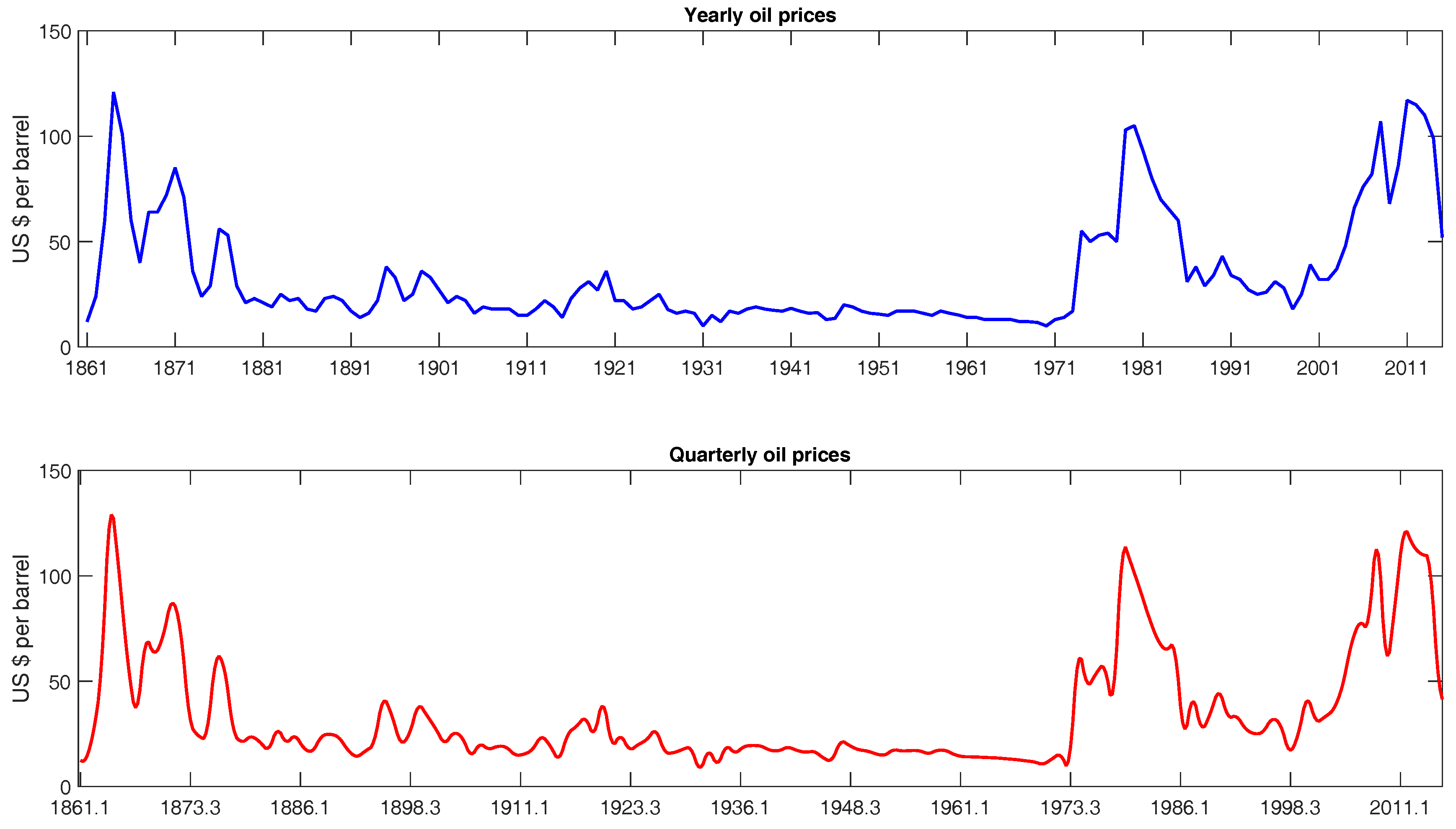
Figure 2.
Oil prices and GDP. Notes: The top figure represents the US real quarterly GDP obtained from the BEA and the NBER (January 1875–February 2016). The bottom figure shows three different real quarterly oil price series: “oilp1” links the BP real quarterly series (transformed using the Chow-Lin technique) with Brent quarterly data from 1957 on; “oilp2” is composed of the BP real quarterly series (transformed using the Chow-Lin technique) and Brent quarterly data from 1970 on; “oilp3” puts together the BP real quarterly series (transformed using the Chow-Lin technique) and Brent quarterly series from 1984 on. Dates are in year.month format.

Figure 3.
Oil prices and GDP growth rates. Notes: The top figure represents the growth rate of the US real quarterly GDP obtained from the BEA and the NBER (January 1875–February 2016). The bottom figure displays the growth rate of “oilp3”, which consists of the quarterly interpolated BP historical dataset until 1956 linked to the quarterly Brent data from 1957 onward and ranges from January 1861 to February 2016. Dates are in year.month format.
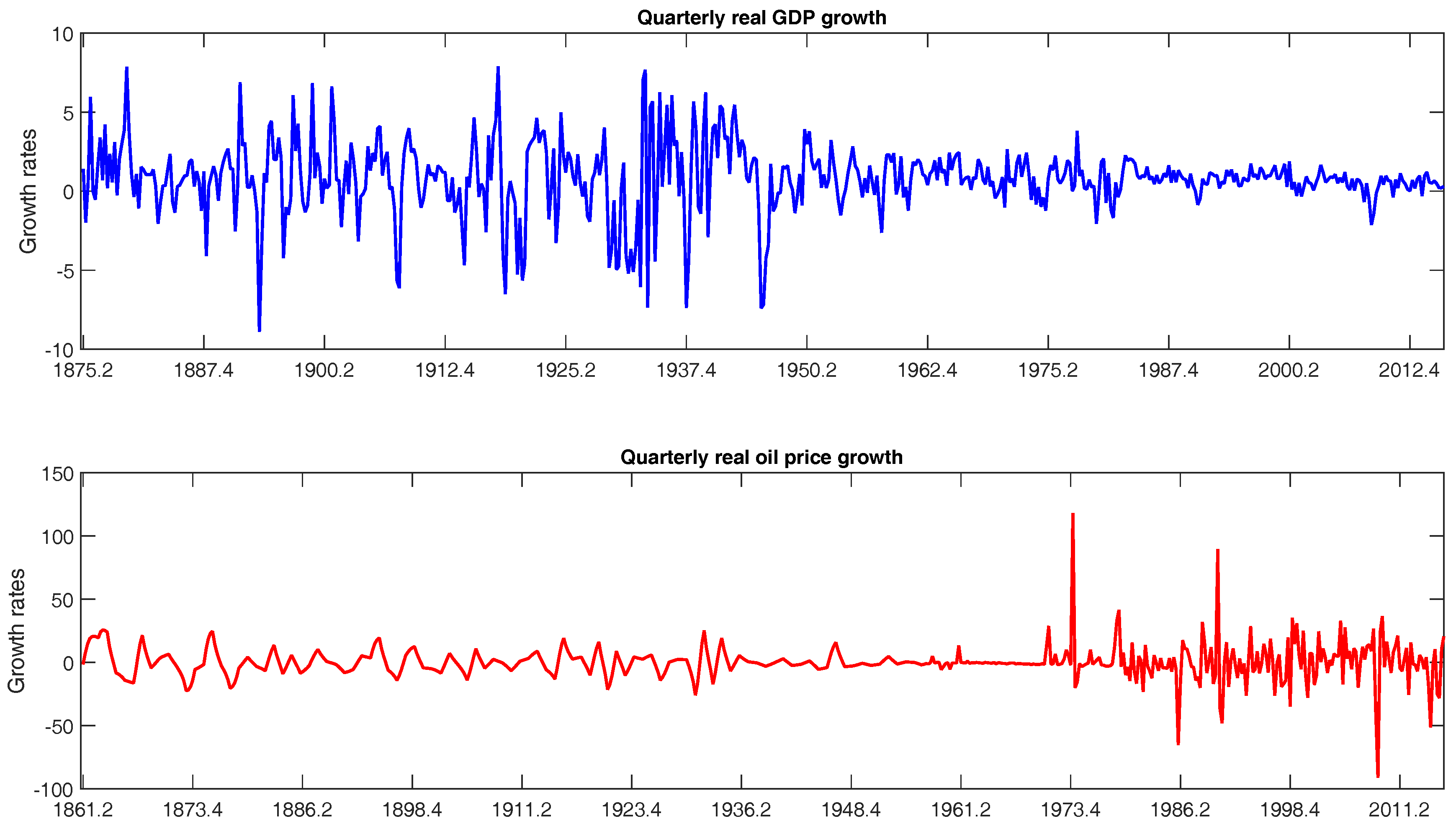
Figure 4.
Impulse-response functions (IRFs) of a VAR(1) for GDP and oil price growth rates. Note: Confidence intervals at 90% of confidence level have been computed according to [33].
Figure 4.
Impulse-response functions (IRFs) of a VAR(1) for GDP and oil price growth rates. Note: Confidence intervals at 90% of confidence level have been computed according to [33].
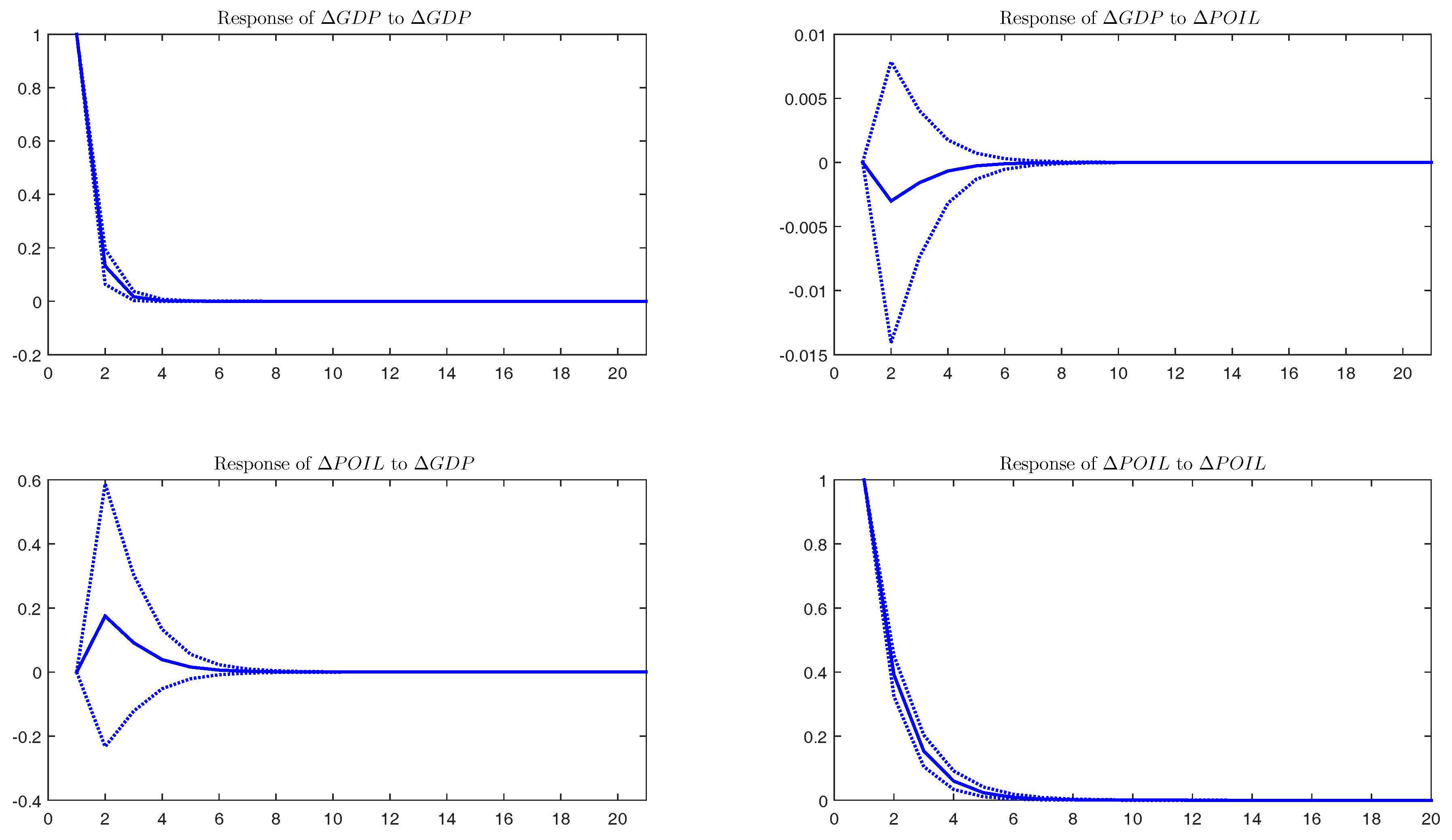
Figure 5.
Rolling estimation of causality test. Notes: We estimate the causality test with a rolling window of 40 quarters. The left-hand side of the figure presents results of Granger causality from to ; the right-hand side shows the results of Granger causality from to . Values in dark blue mean that we can reject the hypothesis of non-causality at 5% significance level and values in yellow mean that we can reject it at 10% significance level, whereas no color indicates no causality between the variables. Dates are in year.month format.

Figure 6.
Rolling estimation of CIR. Notes: We estimate the CIRs with a rolling window of 40 quarters. Confidence intervals at 90% of confidence level. CIR: Cumulative Impulse Response Function. Dates are in year.month format.
Figure 6.
Rolling estimation of CIR. Notes: We estimate the CIRs with a rolling window of 40 quarters. Confidence intervals at 90% of confidence level. CIR: Cumulative Impulse Response Function. Dates are in year.month format.
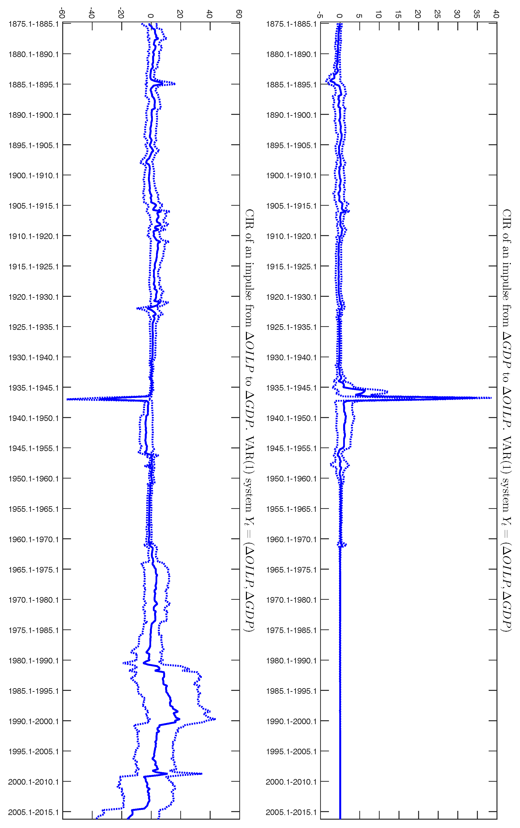
Figure 7.
IRF of February 1875–April 1912. Note: Confidence intervals at 90% of confidence level.

Figure 8.
IRF of January 1913–January 1941. Note: Confidence intervals at 90% of confidence level.

Figure 9.
IRF of February 1941–March 1970. Note: Confidence intervals at 90% of confidence level.

Figure 10.
IRF of April 1970–February 2016. Note: Confidence intervals at 90% of confidence level.
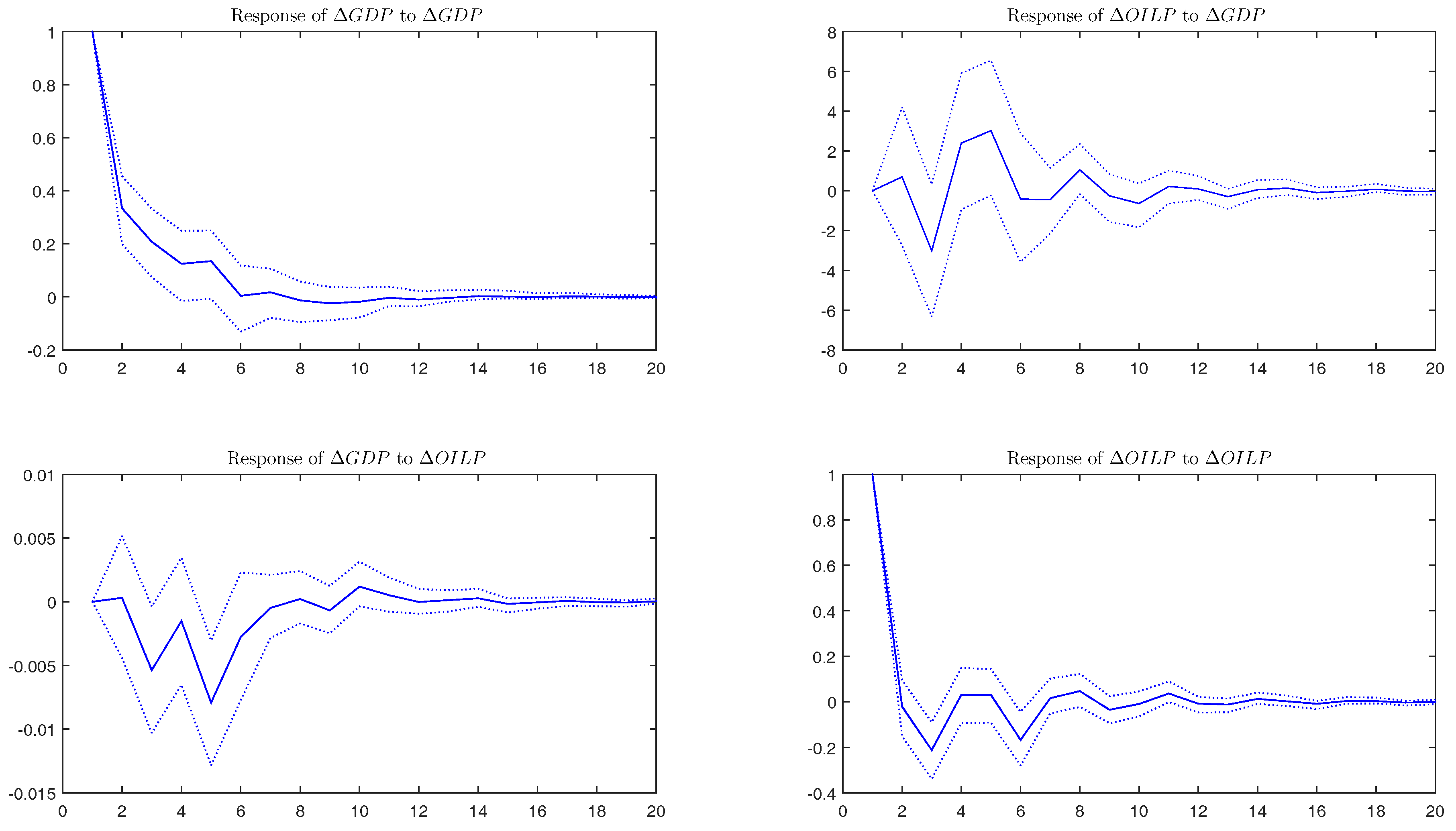
Figure 11.
Posterior means of the standard deviation of residuals.
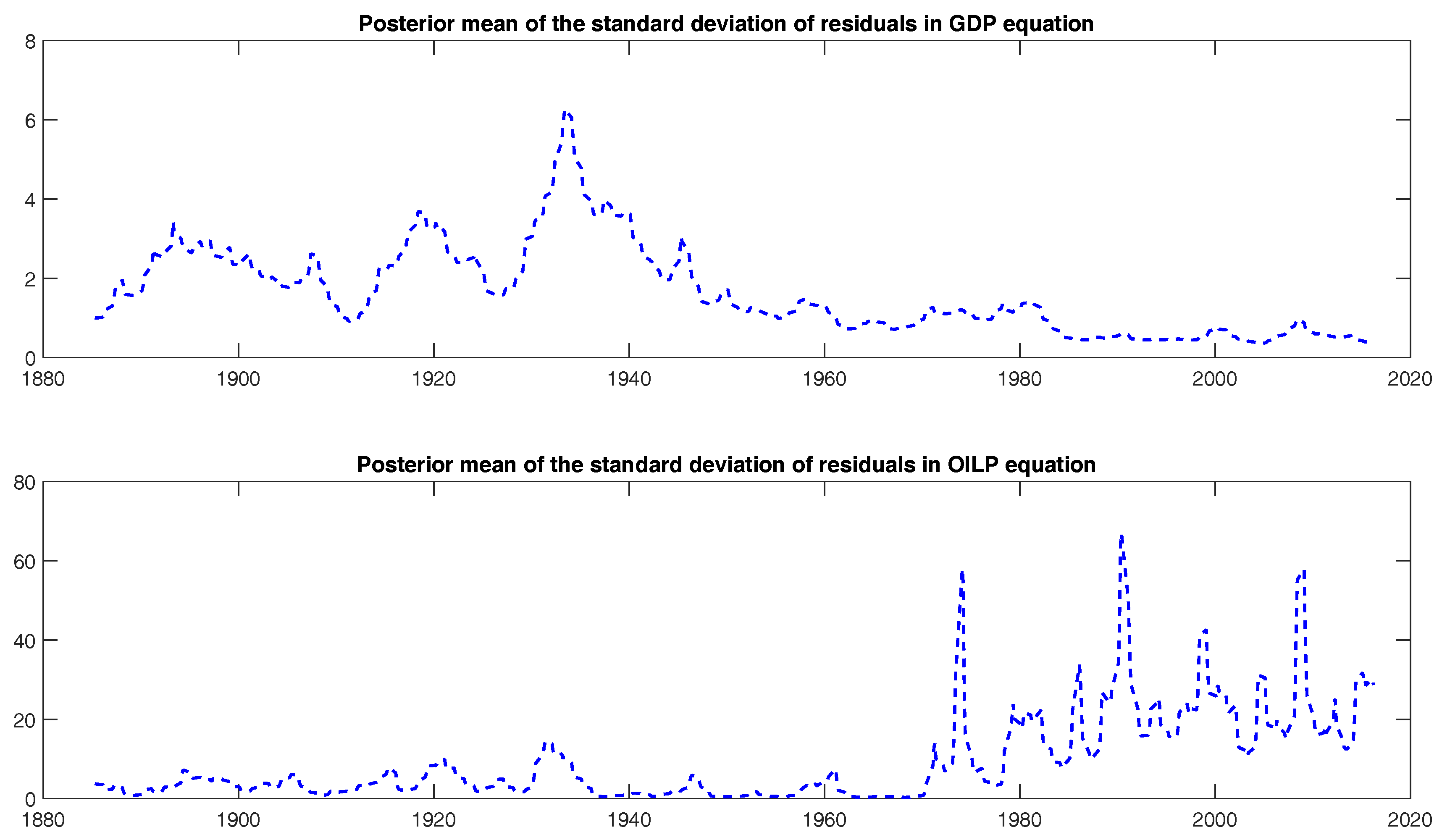
Figure 12.
The five largest downturns and increases of real quarterly oil price.
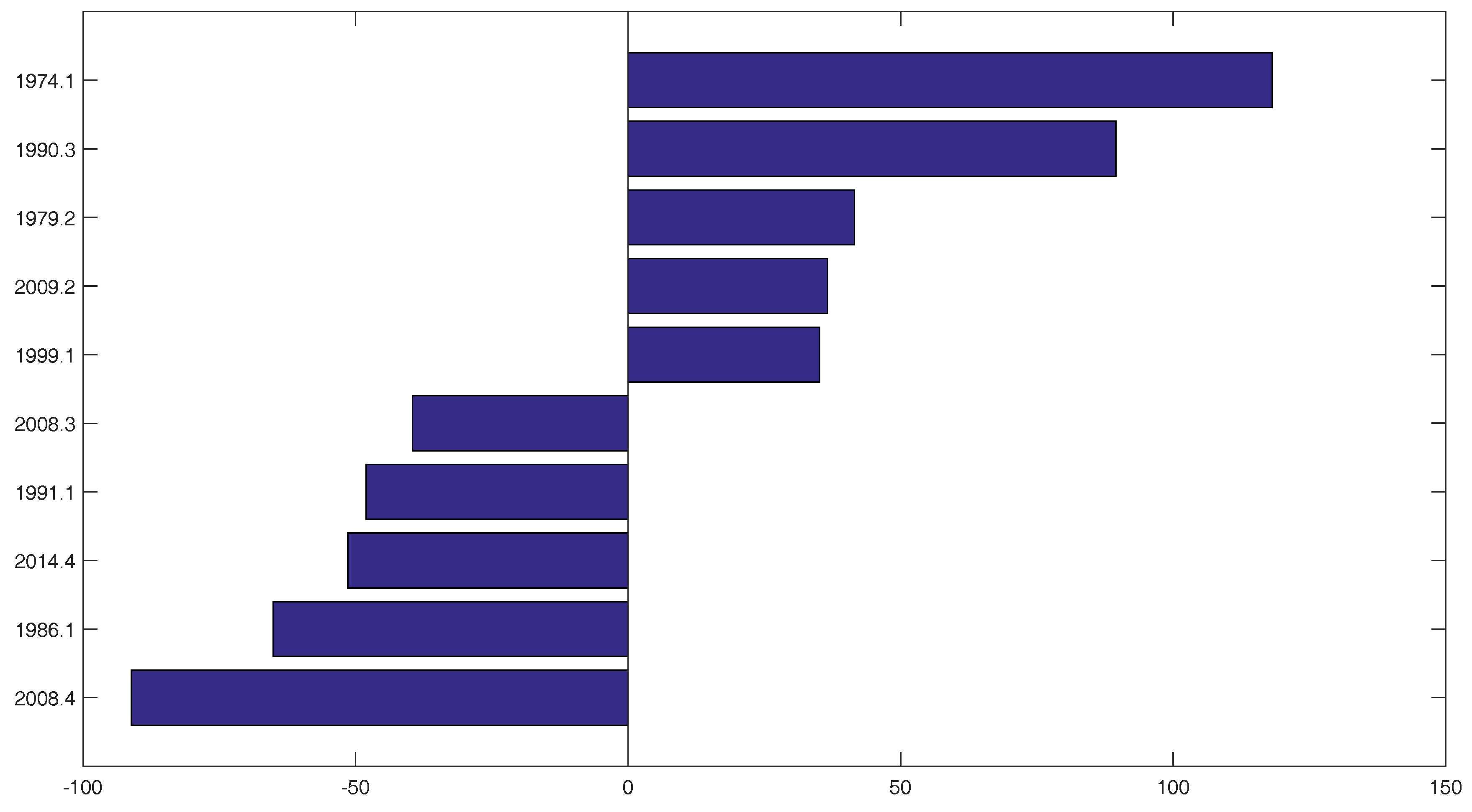
Figure 13.
IRFs to oil price shocks at the time of the five largest increases of oil prices. Note: Confidence intervals at 90% of confidence level.
Figure 13.
IRFs to oil price shocks at the time of the five largest increases of oil prices. Note: Confidence intervals at 90% of confidence level.
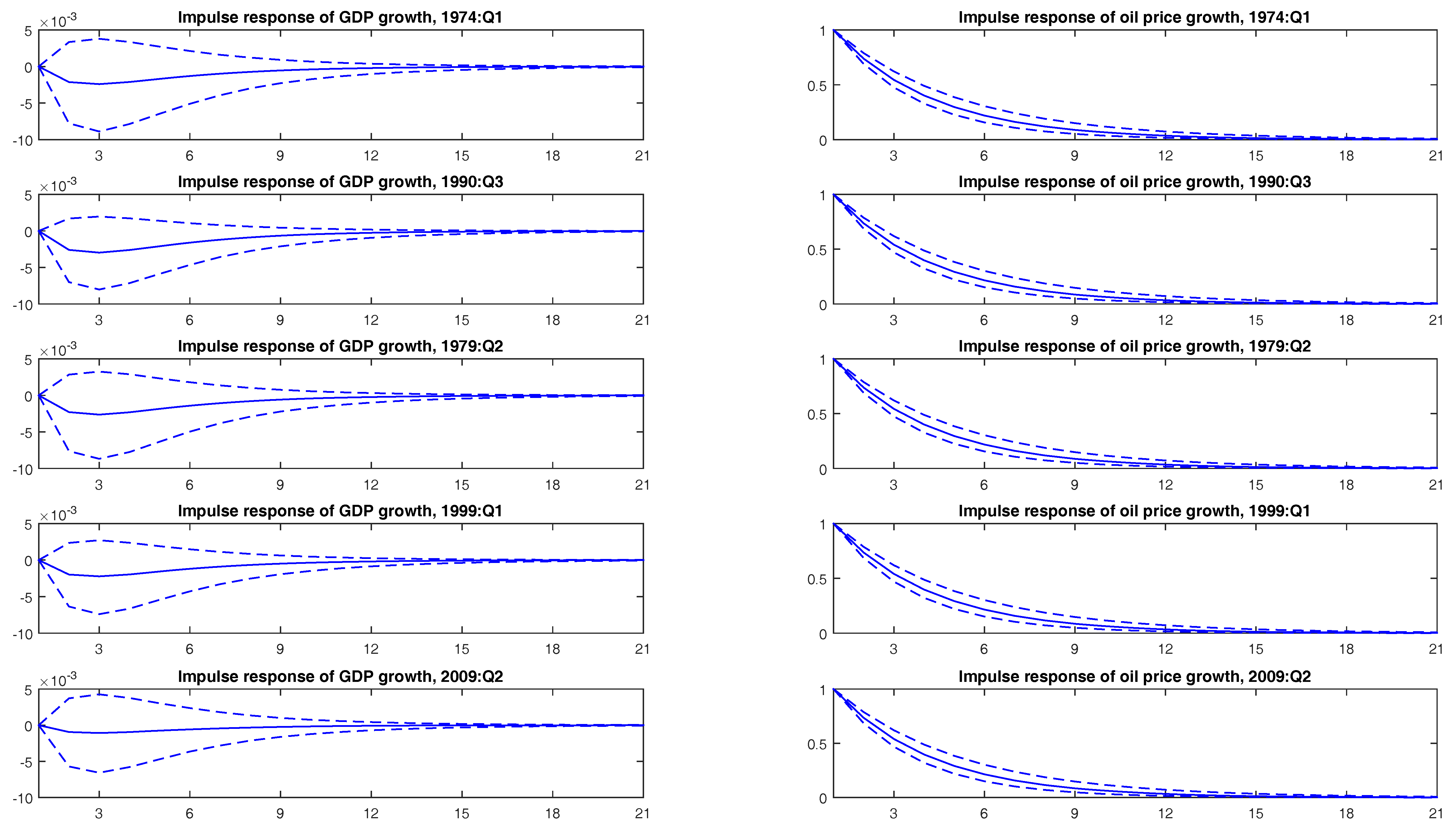
Figure 14.
IRFs to oil price shocks at the time of the five largest decreases of oil prices. Note: Confidence intervals at 90% of confidence level.
Figure 14.
IRFs to oil price shocks at the time of the five largest decreases of oil prices. Note: Confidence intervals at 90% of confidence level.
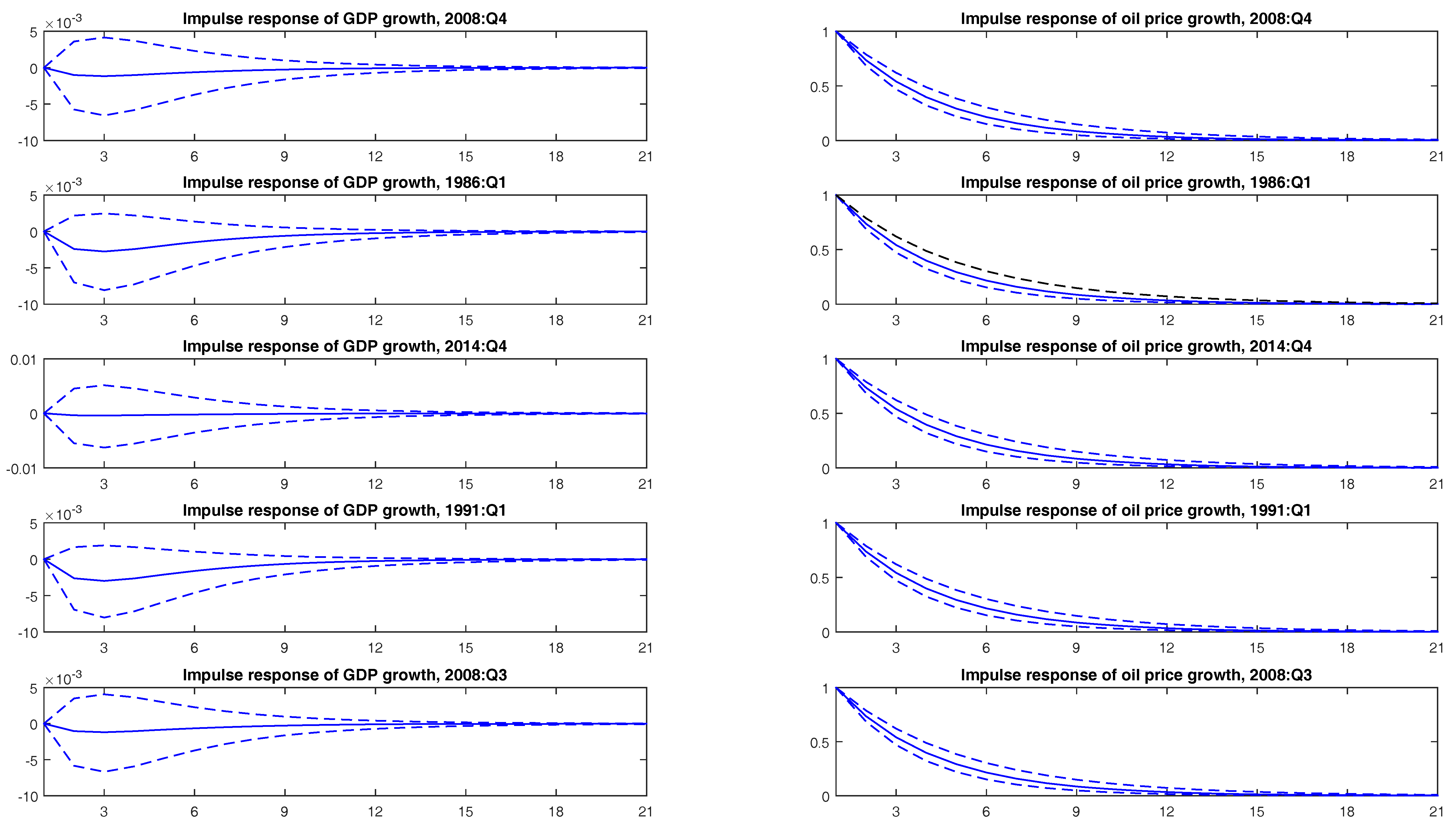
Figure 15.
IRFs of to shocks at the time of the five largest increases of oil prices. Note: Confidence intervals at 90% of confidence level.
Figure 15.
IRFs of to shocks at the time of the five largest increases of oil prices. Note: Confidence intervals at 90% of confidence level.
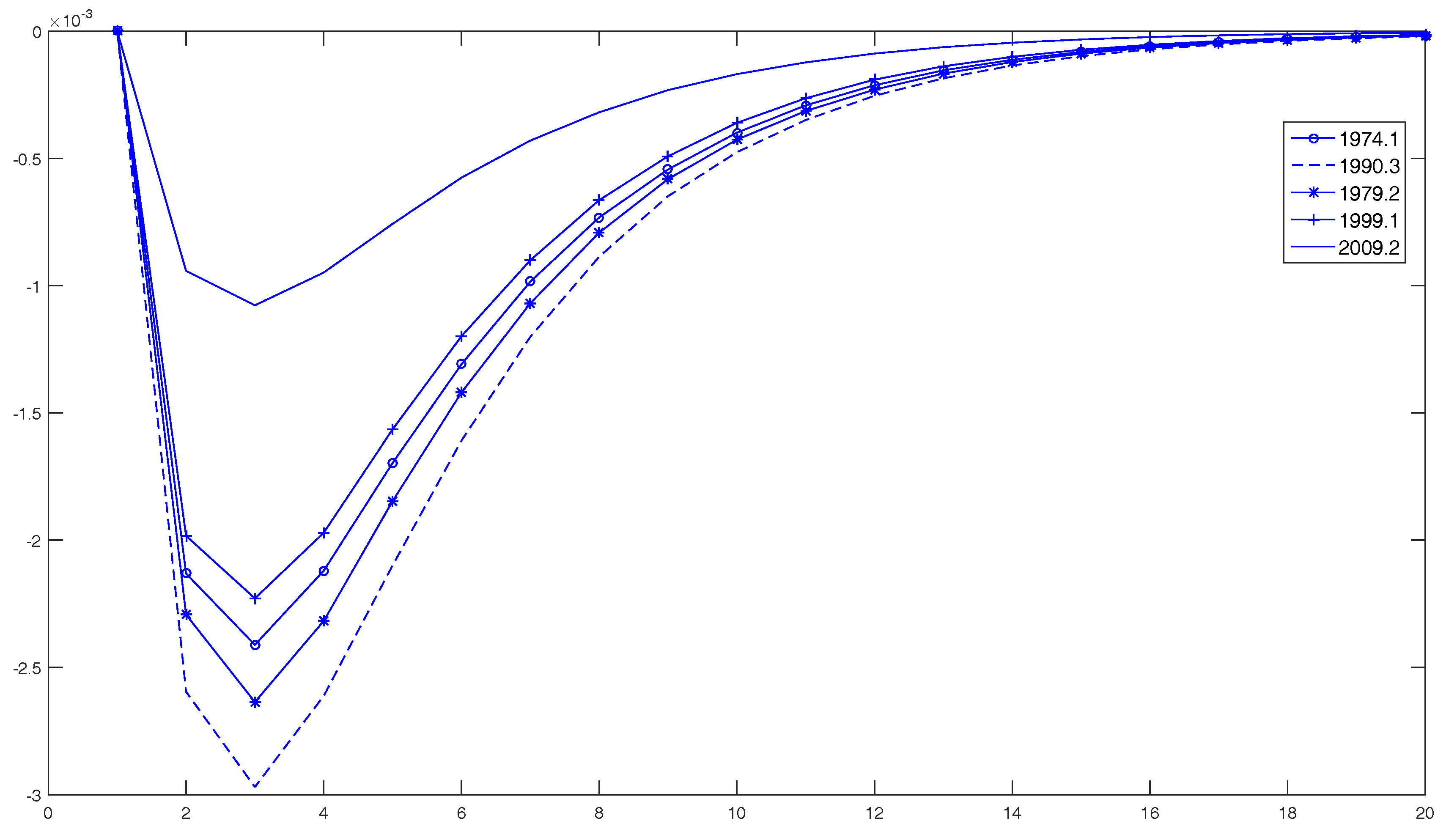
Figure 16.
IRFs of to shocks at the time of the five largest decreases of oil prices. Note: Confidence intervals at 90% of confidence level.
Figure 16.
IRFs of to shocks at the time of the five largest decreases of oil prices. Note: Confidence intervals at 90% of confidence level.

Figure 17.
Comparison of the effects of to shocks at the time of the five largest increases and decreases of oil prices.
Figure 17.
Comparison of the effects of to shocks at the time of the five largest increases and decreases of oil prices.


| ΔGDP | ΔPOIL | |
|---|---|---|
| supF(k) | ||
| k = 1 | ||
| k = 2 | ||
| k = 3 | ||
| k = 4 | ||
| k = 5 | ||
| supF(l + 1/l) | ||
| l = 0 | ||
| l = 1 | ||
| l = 2 | ||
| l = 3 | ||
| l = 4 | − | − |
| UDmax | ||
| WDmax | ||
| T(SBIC) | 0 | 0 |
| T(LWZ) | 0 | 0 |
| T(sequential) | 0 | 0 |
| ΔGDP | ΔOILP | |
|---|---|---|
| ICSS(IT) | ||
| April 1917 | April 1878 | |
| February 1946 | February 1914 | |
| February 1984 | March 1921 | |
| April 2007 | March 1930 | |
| February 2009 | February 1934 | |
| March 1936 | ||
| April 1944 | ||
| March 1947 | ||
| April 1960 | ||
| April 1970 | ||
| ICSS | ||
| March 1929 | January 1862 | |
| March 1934 | January 1963 | |
| February 1946 | April 1878 | |
| January 1984 | March 1930 | |
| February 1934 | ||
| April 1973 | ||
| ICSS | ||
| April 1917 | April 1878 | |
| February 1946 | April 1973 | |
| January 1984 |
Note: Dates of the detected changes in variance. .
| ΔGDP | ΔOILP |
|---|---|
| Model 1 | |
| March 1929 | April 1878 |
| January 1947 | February 1935 |
| February 1984 | April 1973 |
| Model 2 | |
| March 1946 | March 1973 |
| April 1983 | |
Notes: The BP method is applied on the corrected square residuals of , Model 1 or , Model 2. Changes in the mean are tested selecting a trimming of and a maximum number of 10 breaks. Serial correlation and heterogeneity in the errors are allowed. The consistent covariance matrix is constructed using the Andrews method [20]. Critical values in [15].
| Coeff. | p-Value | |
|---|---|---|
| Dependent variable: ΔGDP | ||
| Intercept | 0.486 | 0.000 |
| ΔGDP | 0.392 | 0.000 |
| ΔOILP | −0.003 | 0.649 |
| Dependent variable: ΔOILP | ||
| Intercept | −0.049 | 0.932 |
| ΔGDP | 0.175 | 0.478 |
| ΔOILP | 0.132 | 0.002 |
| Granger causality | ||
| ΔOILPGDP | 0.207 | 0.649 |
| ΔGDPPOIL | 0.504 | 0.478 |
Note: The null hypothesis for the Granger causality test is that does not cause or vice versa.
| WDmax | SupLR | Seq(l + 1/l) | TBi | |||
|---|---|---|---|---|---|---|
| 0 vs. 1 | 0 vs. 2 | 0 vs. 3 | ||||
| 979.130 | 979.130 | 1104.231 | 1159.779 | 156.685 | 64.157 | April 1912, January 1941, March 1970 |
| Granger-Wald causality test | ||||||
| February 1875–April 1912 (6) | January 1913.1–January 1941 (6) | February 1941–March 1970 (5) | April 1970–February 2016 (5) | |||
| ΔOILPGDP | 0.481 | 0.339 | 0.400 | 0.100 | ||
| ΔGDPOILP | 0.251 | 0.272 | 0.000 | 0.497 | ||
Notes: means values significant at 1% level. TB denotes the date of a structural break. The null hypothesis for the Granger causality test is that does not cause or vice versa. We show p-values for the Granger causality test. For each subperiod, we present in brackets the number of lags selected according to several information criteria.
© 2016 by the authors; licensee MDPI, Basel, Switzerland. This article is an open access article distributed under the terms and conditions of the Creative Commons Attribution (CC-BY) license ( http://creativecommons.org/licenses/by/4.0/).
Share and Cite
MDPI and ACS Style
Gadea, M.D.; Gómez-Loscos, A.; Montañés, A. Oil Price and Economic Growth: A Long Story? Econometrics 2016, 4, 41. https://doi.org/10.3390/econometrics4040041
AMA Style
Gadea MD, Gómez-Loscos A, Montañés A. Oil Price and Economic Growth: A Long Story? Econometrics. 2016; 4(4):41. https://doi.org/10.3390/econometrics4040041
Chicago/Turabian StyleGadea, María Dolores, Ana Gómez-Loscos, and Antonio Montañés. 2016. "Oil Price and Economic Growth: A Long Story?" Econometrics 4, no. 4: 41. https://doi.org/10.3390/econometrics4040041
Note that from the first issue of 2016, this journal uses article numbers instead of page numbers. See further details here.