Article

Generalized Fractional Processes with Long Memory and Time Dependent Volatility Revisited

1
School of Mathematics and Statistics, The University of Sydney, Sydney 2006, Australia
2
Faculty of Economics, Soka University, Tokyo 192-8577, Japan
*
Author to whom correspondence should be addressed.
Econometrics 2016, 4(3), 37; https://doi.org/10.3390/econometrics4030037
Submission received: 15 January 2016 / Revised: 3 August 2016 / Accepted: 15 August 2016 / Published: 5 September 2016

Abstract

:
In recent years, fractionally-differenced processes have received a great deal of attention due to their flexibility in financial applications with long-memory. This paper revisits the class of generalized fractionally-differenced processes generated by Gegenbauer polynomials and the ARMA structure (GARMA) with both the long-memory and time-dependent innovation variance. We establish the existence and uniqueness of second-order solutions. We also extend this family with innovations to follow GARCH and stochastic volatility (SV). Under certain regularity conditions, we give asymptotic results for the approximate maximum likelihood estimator for the GARMA-GARCH model. We discuss a Monte Carlo likelihood method for the GARMA-SV model and investigate finite sample properties via Monte Carlo experiments. Finally, we illustrate the usefulness of this approach using monthly inflation rates for France, Japan and the United States.
JEL Classification:
C18; C40; C58

1. Introduction

Consider the well-known ARFIMA ( p , d , q ) model given by:
ϕ ( B ) Y t = θ ( B ) ϵ t ,
where Y t = ( 1 B ) d X t , d ( 1 , 0.5 ) , { ϵ t } is a sequence of uncorrelated (not necessarily independent) random variables, such that V a r ( ϵ t ) = σ 2 , and ϕ ( B ) (stationary AR(p)) and θ ( B ) (invertible MA(q)) polynomials respectively.
This standard case of constant variance innovations has been considered in many traditional time series analysis with applications. However, in recent years, there has been a great number of developments based on time-dependent instantaneous innovation variance (or volatility) such that V a r ( ϵ t ) = σ t 2 . In particular, the following cases have been considered:
(i)
σ t 2 is a deterministic function of t or σ t 2 = f ( t ) ,
(ii)
ϵ t follows the family of (G)ARCH process (see, [1,2]),
(iii)
log ( σ t 2 ) is another stochastic process.
These cases (i) to (iii) can be analysed with emphasis on different practical issues. However, in applications, we need additional assumptions on σ t 2 , such as:
(a)
0 < m < σ t 2 < M < to ensure Var( Y t ) is finite, in (i)
(b)
stationarity or stability of both { ϵ t 2 } and log ( { ϵ t 2 } ) in (ii) and (iii)
Assumption (a) is imposed as it is natural to set bounds for the deterministic function σ t 2 = f ( t ) . In fact, Assumption (b) is required when σ t 2 is a stochastic process. For case (i), the effect of non-stochastic and time-dependent instantaneous variance when d = 0 was studied by Niemi [3] under the standard AR and MA regularity conditions on the zeros of ϕ ( B ) and θ ( B ) , respectively. In his work, Peiris [4] argues that the results of Niemi [3] can be extended to the ARFIMA family when d ( 0.5 , 0.5 ) . In (ii), it is known that X t is strictly stationary if ϵ t is strictly stationary, and in particular, X t is 2 m -th order stationary if ϵ t is 2 m -th order stationary. For the Integrated GARCH (IGARCH) model, Nelson [5] and Bougerol and Picard [6] have argued that IGARCH is strictly stationary under additional regularity conditions. For case (iii) with stochastic volatility, it is obvious that if log σ t 2 is m-th order stationary, then ϵ t is 2 m -th order stationary. Therefore, it can be argued that when σ t 2 is a stationary stochastic process, the conditional likelihood estimation carried out by taking σ t 2 = σ 2 cannot be significant since σ t 2 is bounded. This would be useful in the estimation of parameters, especially in both cases (ii) and (iii). See the survey papers of McAleer [7] and Shephard [8] for the various extensions of (ii) and (iii).
An alternative way of modelling time-dependent volatilities has been extensively studied using ARMA models with time-dependent coefficients driven by constant variance innovations. See, for example, [4,9,10,11,12,13] and the references therein for details. However, this approach is not very attractive in applications, as it involves too many parameters to estimate.
Turning to applications in economic and financial time series, there are many popular directions of modelling and analysis of long-memory. Among others, the analysis of long-memory in inflation has been considered by Backus and Zin [14], Hassler and Wolters [15], Baillie, Chung and Tieslau [16], and Caporale and Gil-Alana [17]. In their paper, Delgado and Robinson [18] considered a number of methods for the analysis of long-memory time series using ARFIMA. An alternative and a general approach is to use the ARFIMA family with conditional and stochastic volatility as considered by Baillie et al. [19], Bollerslev and Mikkelsen [20], Ling and Li [21], Breidt et al. [22], Deo and Hurvich [23], and Bos et al. [24]. In their recent paper, Bos et al. [24] accommodate the stochastic volatility in ARFIMA modelling. Empirical evidence confirms that such models are very satisfactory in practice. Therefore, the aim of this paper is to extend the ARFIMA models with time-varying volatility to a general flexible class of time series models based on Gegenbauer polynomials together with the ARMA structure. The Gegenbauer ARMA (GARMA) model is a generalization of the ARFIMA model. Clearly, the former encompasses the latter as a special case. We will also extend the class of k-factor Gegenbauer process following Woodward et al. [25], Ferrara and Gueganand [26], and Caporale and Gil-Alana [17], by accommodating time-dependent volatility.
The organization of the paper is as follows. Section 2 reviews the family of GARMA with constant variance (volatility). Section 3 shows the existence and uniqueness of second-order solutions for the GARMA model with time-dependent volatility and develops new classes of GARMA-GARCH and GARMA-SV. Section 4 presents the asymptotic results for the maximum likelihood estimator for the GARMA-GARCH model and reports a Monte Carlo likelihood method for estimating the GARMA-SV model. Section 5 presents an illustrative example via simulation data, while Section 6 demonstrate an empirical example using inflation data in France, Japan and the United States. Section 7 gives concluding remarks.

2. Basic Results on GARMA with Constant Volatility

In this section, we review the family of GARMA processes with constant volatility. Based on the work of Gray et al. [27] and Chung [28], consider the family of time series generated by:
ϕ ( B ) ( 1 2 u B + B 2 ) d X t = θ ( B ) ϵ t ,
where the polynomials ϕ ( B ) and θ ( B ) are as defined before, | u | 1 , | d | < 1 are real parameters and ϵ t is white noise with zero mean and variance σ ϵ 2 .
This process in (2) is known as Gegenbauer ARMA of order ( p , d , q ) or GARMA ( p , d , q ; u ) and has the following properties:
  • The power spectrum is given by:
    f X ( ω ) = C ( ω ) × [ 4 ( cos ω u ) 2 ] d , π < ω < π ,
    where C ( ω ) = σ ϵ 2 2 π θ ( e i ω ) ϕ ( e i ω ) 2 and i = 1 .
  • The process in (2) is stationary with long-memory when | u | < 1 and 0 < d < 1 / 2 or | u | = 1 and d < 1 / 4 . The long-memory features are characterized by:
    hyperbolic decay of the autocorrelation function (ACF ) superimposed with a sinusoidal,
    unbounded spectrum at the Gegenbauer frequency, ω = ω g = cos 1 ( u ) .
In their recent papers, a modified class of generalized fractional processes has been studied by Shitan and Peiris [29,30].
Now, consider the following special case or the GARMA ( 0 , d , 0 ; u ) process and its properties for later reference. That is, when ϕ ( B ) = θ ( B ) = 1 , we have:
( 1 2 u B + B 2 ) d X t = ϵ t .
Suppose that the following regularity conditions are satisfied:
  • R1: AR regularity: | u | < 1 and d < 1 / 2 or | u | = 1 and d < 1 / 4 .
  • R2: MA regularity: | u | < 1 and d > 1 / 2 or | u | = 1 and d > 1 / 4 .
A Stationary Solution to GARMA ( 0 , d , 0 ; u ) Model
Under the regularity conditions in R1, there exists the Wold representation to (4) given by:
X t = ψ ( B ) ϵ t = j = 0 ψ j ϵ t j ,
where ψ ( B ) = ( 1 2 u B + B 2 ) d = j = 0 ψ j B j with ψ 0 = 1 and the Gegenbauer coefficients ψ j have the explicit representation:
ψ j = q = 0 [ j / 2 ] ( 1 ) q ( 2 u ) j 2 q Γ ( d q + j ) q ! ( j 2 q ) ! Γ ( d )
such that j = 0 ψ j 2 < ( Γ ( . ) is the Gamma function; see [31] for details). These coefficients ψ j , j 2 are recursively related by:
ψ j = 2 u d 1 + j j ψ j 1 2 d 2 + j j ψ j 2
with initial values ψ 0 = 1 and ψ 1 = 2 d u .
An Invertible Solution to GARMA ( 0 , d , 0 ; u ) Model
Under the MA regularity conditions, there exists an invertible solution to (4) given by:
ϵ t = ( 1 2 u B + B 2 ) d X t = j = 0 π j X t j ,
where π j , j 0 are obtained from (6) replacing d by d with corresponding initial values.
The next section develops the class of GARMA( 0 , d , 0 ; u ) driven by time-dependent or stochastic innovations for later reference.

3. GARMA with Time-Dependent Innovations

Suppose that V a r ( ϵ t ) in (4) is time-dependent. Consider the class of regular (in both AR and MA) GARMA( 0 , d , 0 ; u ) driven by time-dependent innovations satisfying:
ϵ t = σ t z t , z t N I D ( 0 , 1 ) ,
where σ t is the time-dependent volatility.
Below, we establish the existence and uniqueness of second-order solutions to (4) with innovations in (8) under certain additional regularity conditions.

3.1. Unique Stable Solutions

We use the following general approach:
Let ( Ω , A , P ) be a probability space, and let L 0 r ( Ω , A , P ) be the space of all real-valued random variables on ( Ω , A , P ) with finite r-th order moments. Suppose that { ζ t } is sequence of random variables in L 0 r ( Ω , A , P ) and M s ( ζ ) is the closed linear subspace of L 0 r ( Ω , A , P ) spanned by the elements ζ t , t s . Let L 0 r ( Ω , A , P ) be the closed linear subspace spanned by all of the elements ζ t ; t 1 by M ( ζ ) .
In the case of r = 2 , let ξ and ζ be any two random elements in L 0 2 ( Ω , A , P ) such that the inner product and the norm satisfy
< ξ , ζ > = C o v ( ξ , ζ ) and | | ξ | | 2 = E ( ξ 2 )
respectively. It is easy to verify that L 0 2 ( Ω , A , P ) is a Hilbert space.
Intuitively, if the volatility process is stationary, it guarantees the existence of the second moment of ϵ t , which enables us to establish the following two lemmas.
Lemma 1. 
Under the AR regularity conditions R1, if the innovation process is stationary, then the solution in (5) belongs to L 0 2 ( . ) , i.e., X t L 0 2 ( . ) .
Proof. 
Since the innovation process ϵ t is stationary, v a r ( ϵ t ) = σ t 2 is bounded. Hence the solution X t = ψ ( B ) ϵ t = j = 0 ψ j ϵ t j L 0 2 ( . ) .  ☐
Lemma 2. 
Under the MA regularity conditions R2, if the innovation process is stationary, then an invertible solution to (7) belongs to L 0 2 ( . ) or ϵ t L 0 2 ( . ) .
The proof is similar to that of Lemma 1.
Lemma 3. 
Under the both AR and MA regularity conditions and stationarity of the innovation process, one has M t ( X ) = M t ( ϵ ) .
The proof to this follows from Lemmas 1 and 2.
Next, we consider two special cases useful in applications.

3.2. Two Special Cases

Consider two popular cases where the innovations ϵ t follow GARCH or SV processes.

3.2.1. GARMA( 0 , d , 0 ; u)-GARCH( r , s )

Suppose that σ t 2 in (8) follows a GARCH( r , s ) process, such that
σ t 2 = α 0 + i = 1 r α i ϵ t i 2 + j = 1 s β j σ t j 2 ,
where r and s are positive integers (both not simultaneously zero), α 0 > 0 , α i 0 and β j 0 . It is well-known that an equivalent representation of the GARCH( r , s ) process is:
ϵ t 2 = α 0 + i = 1 r α i ϵ t i 2 + j = 1 s β j ϵ t j 2 + η t j = 1 s β j η t j ,
where η t = ϵ t 2 σ t 2 = ( z t 2 1 ) σ t 2 and are serially uncorrelated with mean zero. Now, we state the following lemma:
Lemma 4. 
Let { X t } be generated by GARMA ( 0 , d , 0 ; u ) and σ t 2 follows (9).
(a) 
If the AR regularity conditions and i = 1 r α i + j = 1 s β j < 1 are satisfied, then { X t } is second-order stationary and X t L 0 2 ( . ) .
(b) 
If the MA regularity conditions are satisfied, then { X t } is invertible and ϵ t L 0 2 ( . ) .
Proofs follow from Lemmas 1 and 2.
The next section develops the class of GARMA( 0 , d , 0 ; u ) driven by SV innovations or GARMA-SV.

3.2.2. GARMA( 0 , d , 0 ; u )-SV

Suppose that h t = ln ( σ t 2 ) satisfies the following recursion
ρ ( B ) h t = κ * + ν ( B ) ξ t j ,
where ρ ( B ) = 1 ρ 1 B ρ 2 B 2 ρ l B l and ν ( B ) = 1 + ν 1 B + ν 2 B 2 + + ν m B m , κ * is a constant, ξ t N I D ( 0 , σ ξ 2 ) , and the disturbances z t and ξ t are mutually independent for all t. Further assume that the roots of ρ ( z ) = 0 and ν ( z ) = 0 lie outside the unit circle. Note that σ ξ 2 measures the conditional volatility of the log-volatility.
Let Ψ * ( B ) ρ ( B ) = ν ( B ) . Then, it is known that there exists a sequence { ψ i * } , such that
Ψ * ( B ) = j = 0 ψ j * B j
with j = 0 ( ψ j * ) 2 < . Now, we have the following lemma:
Lemma 5. 
Under the AR regularity condition on ρ ( θ ) , the log-volatility process in (10) has uniquely determined L 0 2 ( . ) solution, such that
h t = κ + j = 0 ψ j * ξ t j ,
where κ = E ( h t ) = κ * ρ ( 1 ) is the mean of the log-volatility process.
It is clear from (11) that the log-volatility process { h t } converges in the mean square to κ and:
E [ ( h t κ ) 2 ] σ ξ 2 j = 0 ( ψ j ) 2 < .
In their paper, Chesney and Scott [32] have considered the case where h t follows an AR(1) process, such that
h t = κ * + ρ h t 1 + ξ t ,
where κ * is a positive constant, and | ρ | < 1 .
Lemma 6. 
The process in (12) is equivalent to
ln ( ϵ t 2 ) = κ ̲ + ρ ln ( ϵ t 1 2 ) + w t ,
where κ ̲ = a ( 1 ρ ) + κ * , a = E [ ln ( z t 2 ) ] = 1.2704 , w t = u t ρ u t 1 + ξ t and u t = ln ( z t 2 ) a . Note that E [ w t ] = 0 ; V a r [ w t ] = 4.93 ( 1 + ρ 2 ) + σ ξ 2 ; E ( w t w t 1 ) = ρ ; E ( w t w t j ) = 0 ( j 2 ) .
Proof. 
Since ln ( ϵ t 2 ) = ln ( σ t 2 ) + ln ( z t 2 ) , we have ln ( ϵ t 2 ) = h t + ln ( z t 2 ) . Substituting for h t = ln ( ϵ t 2 ) a u t in (12) and noting that V a r [ ln ( z t 2 ) ] = 4.93 , the lemma follows. ☐
Remark. 
Clearly, { w t } in (12) is not a martingale difference series, and hence, it is not useful in applications. However, this can be written as an ARMA(1,1) in the form:
ln ( ϵ t 2 ) = κ ̲ + ρ ln ( ϵ t 1 2 ) + v t θ v t 1 ,
where v t W N ( 0 , σ v 2 ) ; θ and σ v 2 are given by 1 + θ 2 θ = ( 1 + ρ 2 ) σ u 2 + σ ξ 2 ρ σ u 2 , σ u 2 = V a r [ log ( z t 2 ) ] = 4.93 .
This result can be extended to any general ARMA structure for the log-volatility process.
Lemma 7. 
Suppose that the SV process follows an ARMA( l , m ) model as in (10). Then, the corresponding { ln ( ϵ t 2 ) } process satisfies and ARMA ( k , k ) in the form:
ln ( ϵ t 2 ) = κ ̲ + ρ 1 ln ( ϵ t 1 2 ) + ρ 2 ln ( ϵ t 2 2 ) + + ρ k ln ( ϵ t k 2 ) + v t + θ 1 v t 1 + + θ r v t k ,
where κ ̲ = κ * + a ( 1 ρ 1 ρ 2 ρ p ) and v t = ξ t u t , v t j = θ j ξ t j ρ j u t j for j = 1 , 2 , , k with k = max ( l , m ) .
Proof. 
The proof follows from extending the approach in Lemma 6. ☐
Section 4 discusses the estimation of parameters.

4. Estimation of Parameters

This section discusses the estimation for the GARMA (p,d,q; u) model with time-dependent volatility. We divide the section into to two parts, namely, (i) the GARMA-GARCH and (ii) the GARMA-SV.

4.1. GARMA-GARCH Model

Suppose that X = { X 1 , , X n } is generated by the GARMA (p,d,q; u)-GARCH(r,s) model (2), (8) and (9). Define ϕ = ( ϕ 1 , , ϕ p ) , θ = ( θ 1 , , θ q ) , α = ( α 0 , α 1 , , α r ) , β = ( β 1 , , β s ) , γ = ( d , ϕ , θ ) and δ = ( α , β ) . Let λ = ( u , δ , γ ) , and let λ 0 = ( u 0 , δ 0 , γ 0 ) be the true value of λ in the interior of the compact set Λ. The approximate log-likelihood function (excluding the constant) is given by
L ( λ ) = 1 n t = 1 n l t , l t = 1 2 log ( σ t 2 ) ϵ t 2 2 σ t 2 ,
where
ϵ t = [ θ ( B ) ] 1 ϕ ( B ) ( 1 2 u B + B 2 ) d X t , σ t 2 = [ β ( B ) ] 1 [ α 0 + α ( B ) ϵ t 2 ]
and α ( B ) = α 1 B + α 2 B 2 + + α r B r , β ( B ) = 1 β 1 B β 2 B 2 β s B s .
Assuming the initial values of X 0 , X 1 , X 2 , are zero, an approximate maximum likelihood estimator λ ^ of λ in Λ is obtained by maximizing the above function, which is asymptotically equivalent to the maximum likelihood (ML) estimator. For the case of a non-normal distribution, we can still use the same approach with the corresponding quasi-maximum likelihood (QML) estimator.
For the ARFIMA ( p , d , q )-GARCH ( r , s ) model, Breidt et al. [22] suggested the above approach. However, Ling and Li [21] established the consistency and asymptotic normality of the corresponding ML estimator and showed that the information matrix is block-diagonal. Combining the results of Ling and Li [21] and Chung [28,33], we can obtain the asymptotic results for the corresponding estimator of the GARMA-GARCH model.
Proposition 1. 
Let u ^ and ( γ ^ , δ ^ ) be approximate ML estimators of u and ( γ , δ ) based on a sample { X t } t = 1 n from a GARMA-GARCH model under the conditions in Lemma 4. Then, u ^ is asymptotically independent of ( γ ^ , δ ^ ) and:
n ( u ^ u 0 ) L K sin ( ω g ) d Y 0 i f   | u | < 1   a n d   d 0 ,
where K = E ( σ t 2 ) + 2 j = 1 φ σ ( j ) E ( ϵ t i 2 / σ t 4 ) ,
Y 0 0 1 W ˜ 1 d W 2 0 1 W 1 d W ˜ 2 0 1 W ˜ 1 2 ( r ) d r + 0 1 W 1 2 ( r ) d r
and ( W ˜ 1 ( t ) , W ˜ 2 ( t ) ) and ( W 1 ( t ) , W 2 ( t ) ) are two independent Brownian motions with mean zero and covariance
t E ( σ t 2 ) 1 1 K .
Furthermore,
n 2 ( u ^ 1 ) L ± K 2 d Y 1 i f   u = ± 1   a n d   d 0 ,
where Y 1 is a random variable defined as
Y 1 0 1 0 r W 1 ( s ) d s d W 2 ( r ) 0 1 0 r W 1 ( s ) d s 2 d r .
Proof. 
See Appendix A.2. ☐
As discussed in Chung [28,33], the convergence rates of u ^ are faster than those of the remaining parameters. The off-diagonal blocks in the information matrix (with respect to the parameter u and the remaining parameters) approach zero. Hence, the distribution of u ^ is asymptotically independent of the remaining parameters.
Below, we report the asymptotic result of the remaining parameters.
Proposition 2. 
Based on the sample { X t } t = 1 n from the GARMA-GARCH model and under the conditions in Lemma 4, we have
n γ ^ γ 0 δ ^ δ 0 L N 0 , Ω γ 1 O O Ω δ 1 ,
where u 1 and
Ω γ = E 1 σ t 2 ϵ t γ ϵ t γ + 1 2 σ t 4 σ t 2 γ σ t 2 γ , Ω δ = E 1 2 σ t 4 σ t 2 γ σ t 2 γ .
Proof. 
See Appendix A.3. ☐
For the case of u to be one, we can use the asymptotic result of Ling and Li [21].
Following Gray et al. [27] and Chung [28], in practice, we use the grid search procedure for different value of u over the range [ 1 , 1 ] to minimize the likelihood function. For selecting the order of the GARMA-GARCH model, we can use an information criterion, such as AIC and BIC. Furthermore, we can use the conventional t test for the parameters except for u. For testing the null hypothesis regarding u, we can use the approach of Chung [33] to obtain percentiles via simulations.

4.2. Estimation of GARMA-SV Model

Suppose that X = { X 1 , , X n } are generated from the GARMA (p,d,q; u)-SV model (2), (8) with the SV structure
h t = κ + ρ ( h t 1 κ ) + ξ t , | ρ | < 1 ,
where h t = ln ( σ t 2 ) , { ξ t } N I D ( 0 , σ ξ 2 ) and ξ t , z t are independent.
From (18), we have E ( h t ) = κ and V a r ( h t ) = σ ξ 2 1 ρ 2 . Further, V a r ( ϵ t ) = exp σ ξ 2 2 ( 1 ρ 2 ) . Since { h t } is a latent process, the evaluation of the likelihood function requires integrating it with respect to ( h 1 , , h n ) .
As mentioned earlier, the evaluation of the likelihood function involves high-dimensional integration, which is difficult to calculate. Nevertheless, among others, Danielsson and Richard [34], Shephard and Pitt [35], Durbin and Koopman [36,37] and Liesenfeld and Richard [38] suggested evaluating high-dimensional integrals using simulation methods and then maximizing the corresponding likelihood function. In this case, we use the Monte Carlo likelihood (MCL) estimator of Durbin and Koopman [37]. In their recent paper, Bos et al. [24] extended the MCL estimator for the estimation of parameters of ARFIMA-SV parameters. This approach creates a set of realized values for h = ( h 1 , h 2 , , h n ) by ‘importance sampling’. Conditional on h and using the prediction error decomposition, it is clear that the density is given by:
log ( X | h , d , ϕ , θ , κ . ρ , σ ξ ) = n 2 log ( 2 π ) 1 2 t = 1 n log ( f t ) 1 2 t = 1 n a t 2 f t ,
where a t is the one-step ahead prediction error, f t is its variance and h is from importance sampling.
From (19), we evaluate the simulated likelihood function based on the true density and the importance density using the results of Durbin and Koopman [37]. We also extend the work of Bos et al. [24], by replacing the autocovariance functions of the ARFIMA by those of the GARMA and use the results of McElroy and Holan [39] to obtain the ML estimator. As a practical issue, we use the grid search procedure for different values of u over the range [ 1 , 1 ] for minimizing the likelihood function.
Noting that h t / u = 0 , h t / γ = 0 , we can consider that the information matrix of ( u , γ , δ 2 ) has a block diagonal structure similar to the GARMA-GARCH case, where δ 2 = ( κ , σ ξ , ρ ) . If the MCL approximates the true likelihood accurately, we can use the conventional t test for the parameters except for u. For testing the null hypothesis regarding u, we can use the approach of Chung [33] to obtain percentiles via simulations, based on Proposition 1. For this purpose, we need to replace K in Proposition 1 with K * = E [ exp ( 2 h t ) ] , by noting h t / u = 0 unlike the GARMA-GARCH process.
In the next section, we will investigate the finite sample properties of the MCL estimator. In selecting the order of the GARMA-SV model, we can use the MCL to calculate the information criterion, such as AIC and BIC.
It is worth mentioning a semi-parametric estimation procedure for the long-memory parameter under heteroskedasticity. See, for example, [40]. For the GARMA-SV model, we extend this in two directions: one is to to replace the conditional heteroskedasticity by SV, and the other is to extend the ARFIMA to the GARMA. For the latter case regarding the GARMA process, Hidalgo and Soulier [41] developed a log-periodogram regression estimator extending the work of Robinson and Henry [40].
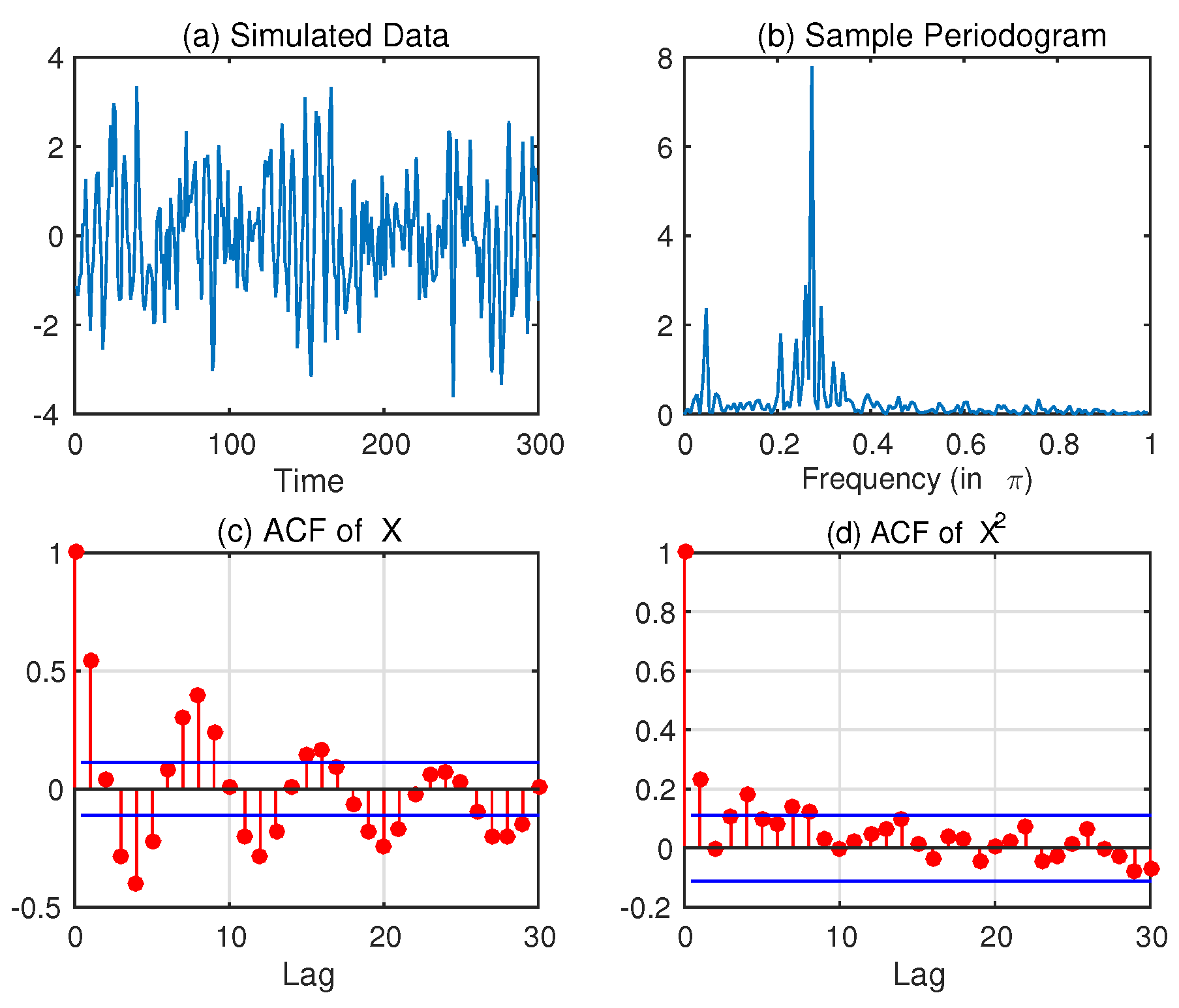
Now, look at a simulation study in order to illustrate certain properties of this GARMA-SV class.

5. Simulation Results

In this section, we show two kinds of simulation results for the GARMA-SV model. One is an illustrative example to show the pattern of a GARMA-SV process, and the other is the Monte Carlo results for the finite sample properties of the ML estimator for the GARMA-SV.

5.1. An Illustrative Example

We generate a one-shot series to show as an illustrative example. Simulate 500 values from GARMA( 0 , d , 0 ; u )-SV from (4) and (8) with SV innovations as in (15). We have selected the parameter values ( u , d ) = ( 0.7 , 0.3 ) for the following two cases:
  • Case (i) with constant volatility: ( κ , ρ , σ ξ ) = ( 0 , 0 , 0 ) ,
  • Case (ii) with stochastic volatility: ( κ , ρ , σ ξ ) = ( 0 , 0.98 , 0.2 ) .
Take the time series of 300 observations (discarding the first 200) for further analysis. It is clear that the Gegenbauer frequency is ω G = 0.2532 π = 0.7954 .
For the simulated GARMA( 0 , d , 0 ; u ), Figure 1 shows the time series plot, the sample periodogram and the autocorrelation functions (ACF) of series. In addition, 95% confidence intervals for the squared series are presented. The periodogram indicates that the peak is at ω = 0.2733 π , which is close to the actual value. The ACFs of the raw series decay hyperbolically and periodically, confirming the features of the Gegenbauer process. On the other hand, the ACFs of the squared series are insignificant for higher lags.
Figure 2 presents the plots for a simulated GARMA( 0 , d , 0 ; u )-SV process. The time series plot indicates the pattern of the time-dependent volatility. Figure 2b shows three major peaks at frequencies of 0.0467π, 0.1600π and 0.2733π. Clearly, the last peak is close to the true Gegenbauer frequency. Figure 2c shows that the ACF of the raw series decays hyperbolically and periodically (similar to the result in Figure 1c of the Gegenbauer process). The ACF in Figure 2d shows a geometric decay, which is different from Figure 1d, which shows constant volatility.
As shown in Figure 1b, the periodogram of the GARMA process has one major peak at the Gegenbauer frequency, which is further from the origin. These plots show that there is a possibility of having multiple peaks under the time-dependent volatility model. The next section gives an empirical study based on a monthly consumer price index as an example.

5.2. Monte Carlo Experiments

In order to examine the finite sample properties of the MCL estimator for the GARMA-SV model, we conduct a simulation study. For the ARFIMA-SV model, Bos et al. [24] conducted Monte Carlo experiments for the MCL estimator for the ARFIMA ( 1 , d , 0 )-SV model, and found (i) downward bias in d, (ii) upward bias in φ, (iii) downward bias in ρ and (iv) upward bias in σ ξ , with the sample size T = 500 . We consider the GARMA ( 1 , d , 0 ; u )-SV model in order to check the effects of the additional parameter u. As explained in the previous section, we use the grid-search for estimating u over the interval [ 1 , 1 ] .
We specify the parameters for the GARMA part as ( μ , d , u , ϕ ) = ( 0.1 , 0.4 , 0.7 , 0.384 ) , implying that the value of the first-order autocorrelation function is 0.6. For the parameters for the SV part, we use the values ( κ , ρ , σ ξ ) = ( 7.36 , 0.95 , 0.26 ) , which are used in the simulation experiments of Jacquier et al. [42]. We consider a sample size of T = 500 with 2000 replications.
Table 1 shows the sample means, standard deviations and root mean squared errors (RMSE) of the MCL estimators. For the parameter u, the bias and RMSE are smaller than those for d and ϕ 1 , implying a faster convergence rate for the MCL estimator of u, as expected from Theorem 1 of Chung [33], for the simple GARMA process and from Proposition 1 of the current paper for the GARMA-GARCH model. Figure 3 shows the estimated density of the u ^ , indicating that 94% of the estimates are located between (0.65,0.75) and that 2.8% of them are greater than 0.95. For the remaining parameters, Table 1 agrees with the simulation results of Bos et al. [24], except for ϕ 1 . The MCL estimator for ϕ 1 gives a downward bias, which may be explained by the fact that not only ( d , ϕ 1 ) , but also u , affect the autocorrelation structure of the GARMA part.

6. Applications of GARMA-SV Models

We use the monthly consumer price index (CPI) P t in three countries: France, Japan and the United States (U.S.) to illustrate the modelling described in this paper. The sample period starts from 1960M11 to 2015M11 in all three countries. The data source is the IMF’s International Financial Statistics published on the IMF web page. The CPIs are normalized at 100 for the year 2010. >From the price index series, we calculate the monthly inflation rates, Π t = 100 × log ( P t / P t 1 ) giving T = 660 observations. By removing the seasonal effects, regress the inflation rates on a series of monthly dummies D t as Π t = D t δ ̲ + e t . Define X t = Π ¯ + e ^ t , where Π ¯ is the average of inflation rates and e ^ t is the residuals through the method of OLS. 
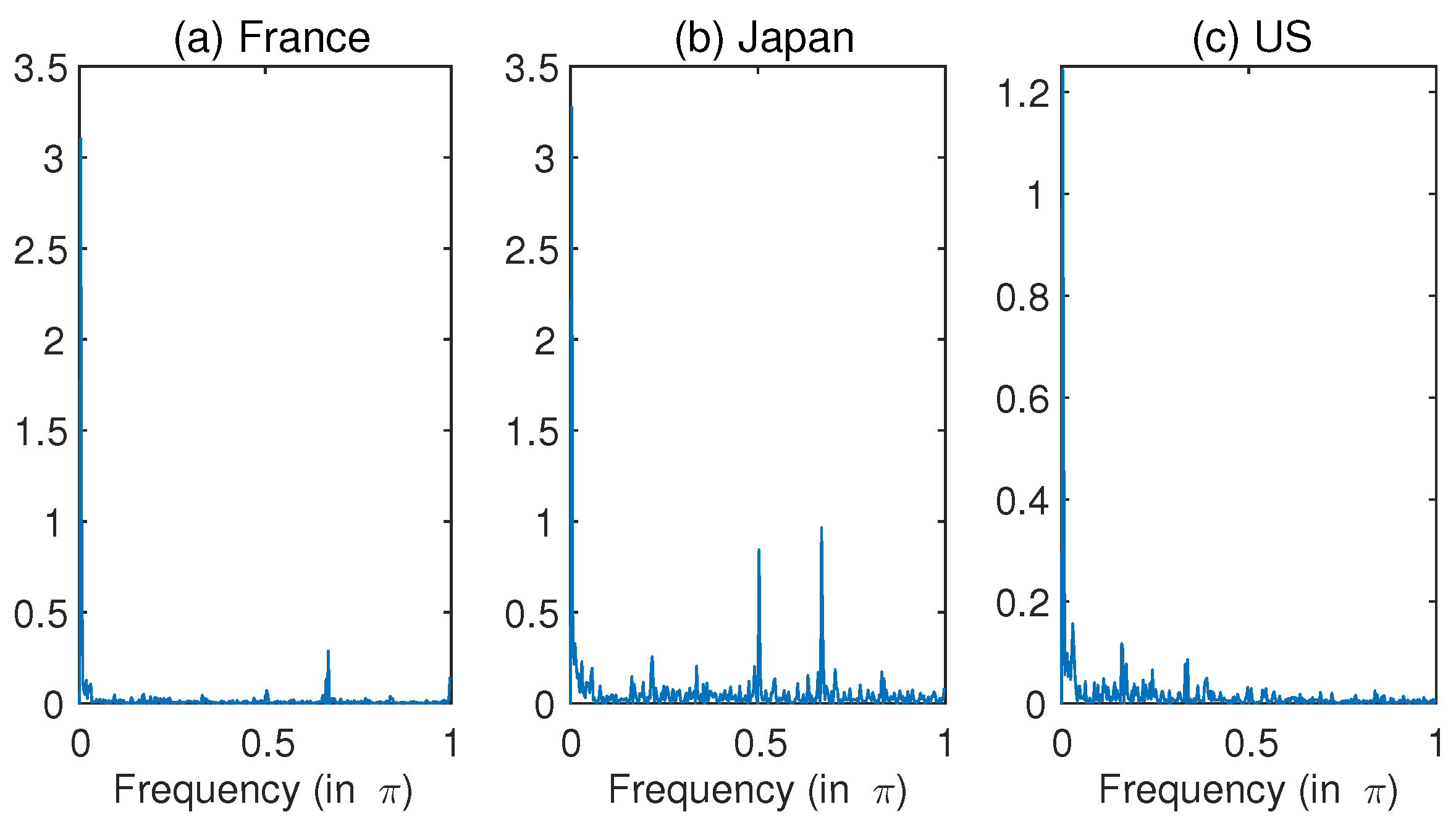
Table 2 shows the corresponding descriptive statistics. For seasonally-adjusted inflation rates, Figure 4 shows the estimated periodograms. As in Figure 4, the highest peak is at ω = 0.0033 π for all three countries. Apart from the pole, there are at least two small peaks. The second highest peak is at ω = 0.6697 π for France and Japan, while the peak in the second mass is at ω = 0.1606 π for the U.S. Although it is difficult to distinguish, the third highest peak for France is at ω = 0.9970 π . Based on the ACF and spectral properties, we examine the reasons for these multiple peaks. The first candidate is time-dependent volatility as discussed in the previous section. The second one is the general GARMA process with multi-factors, and the third is a nested model of the multi-factor GARMA and the SV.
In this case, we estimate the three-factor GARMA-SV model given by:
( 1 ϕ L ) ( 1 2 u 1 B + B 2 ) d 1 ( 1 2 u 2 B + B 2 ) d 2 ( 1 2 u 3 B + B 2 ) d 3 X t = ϵ t ,
based on (8) and (18) and using the MCL estimation technique. By the sample periodogram in Figure 4, we expect that one of the three Gegenbauer frequencies is zero, corresponding to the highest peak at the point close to the origin. We do not report the higher orders of ( p , q ), as the estimates were insignificant (using the mean subtracted series following the recommendation of Chung [28]). The estimates of d i are located in (0.05, 0.2) and are significant at five percent, except for d 2 for the U.S. series. For all three countries, the null hypothesis of u 1 = 1 cannot be rejected. A positive value of u i indicates that the Gegenbauer frequency is close to the origin, while a negative value implies that it is close to π. Hence, the Gegenbauer frequency for U.S. data is close to the origin, while the estimates of ( u 2 , u 3 ) of the other two countries are close to π. It is interesting to note that the estimates of 
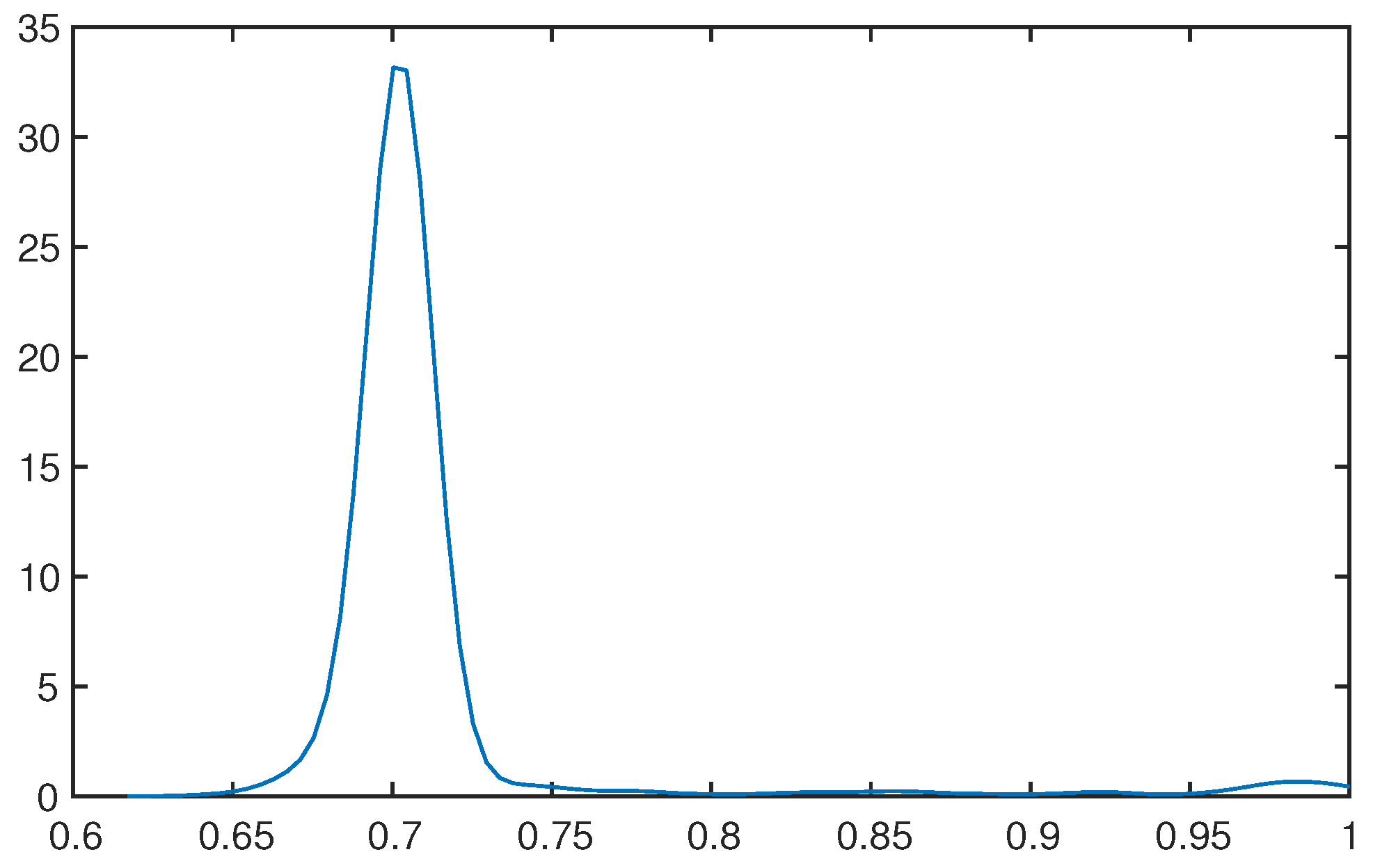
ρ are positive and significant, indicating the appropriateness of accommodating the time-dependent volatility structure in this multi-factor GARMA model. The empirical results support this three-factor GARMA-SV model for France and Japan, while the U.S. series favours the two-factor GARMA-SV model.
Since the estimates of ρ are close to one for Japan and the U.S. series, we consider a GARMA model for the SV process, { h t } . Using the MCL estimates from Table 3, we obtain the residuals to satisfy
ϵ ^ t = ( 1 2 u ^ 3 B + B 2 ) d ^ 3 ( 1 2 u ^ 2 B + B 2 ) d ^ 2 ( 1 2 u ^ 1 B + B 2 ) d ^ 1 ( 1 ϕ ^ L ) X t .
Now, we consider the interpretation of the parameter u i . First of all, the behaviour of a periodic long-memory process is different from a periodic short memory process (for example, a seasonal ARMA). As shown by Chung [28,33], the j-th autocovariance function for the GARMA process is approximated by K j 2 d 1 cos ( ω g j ) , where K is a constant. Hence, the operator ( 1 u i B + B 2 ) d i produces a periodic long-memory with cycles of every 2 π / arccos ( ω g , i ) . For France, the values for i = 2 , 3 are 2.986 and 2.018, respectively. These results indicate that there are periodic long-range dependences with respect to every two and three months. The values of Japan are 2.986 and 3.976, implying the periodic long-memory with respect to every three and four months. For the U.S., the estimate for u 3 is 5.946, producing the periodic long-memory with respect to every six months. As u 1 is equal to one in three countries, there is no periodic long-memory for the first factor.
Figure 5 shows the periodograms for the log of the squared residuals, log ϵ ^ t 2 , which can be considered as the proxy of log-volatility. Figure 5 shows that there is a distinguished peak at zero frequency for the case of Japan and the U.S., implying that a short memory model model is adequate for France, while long-memory models are appropriate for the remaining two countries. Furthermore, Japan also has five other periodic peaks, implying a multiple periodic long-memory. For estimating the GARMA-SV model when h t follows a GARMA model, the MCL technique requires a smoother simulation to be applied to the second GARMA process, which is an extension of the work of de Jong and Shephard [43]. Another task is to reduce the computational time under the multiple grid-search method for finding optimal values of u i ’s in mean and volatility. We need to wait for further research for these problems.
In this section, we found that in addition to non-periodical long-range dependence, the empirical results indicate the existence of the periodic long memory under the time-dependent volatility.

7. Conclusions

This paper considers the class of GARMA-GARCH and GARMA-SV models in detail. We have established the existence and uniqueness of second order solutions and investigated the asymptotic results of the approximated ML estimator for the GARMA-GARCH model. We have explained the Monte Carlo likelihood (MCL) technique for estimating the GARMA-SV model. Using a set of simulated data, we have presented an illustrative example with possible multiple peaks in the GARMA-SV model. We also conducted a Monte Carlo experiment to investigate finite sample properties of the MCL estimator. In the empirical analysis, we have estimated a three-factor GARMA-SV model for monthly inflation rates of France, Japan and the United States and found that the data favour multi-factor GARMA-SV models showing that periodic long-memory exists.
There are many possible extensions of this new approach. In a future paper, we will develop models allowing both the mean and variance to follow Gegenbauer processes, as discussed in the previous section. For this purpose, we may extend the MCL estimation method by considering the simulation smoother for the GARMA process. By extending the work of Robinson and Henry [40], we plan to develop an estimation method for the Gegenbauer frequency and the long-memory parameter in the presence of long-memory in volatility.

Acknowledgments

The authors are most grateful to the editor, Kerry Patterson, and five anonymous reviewers for very helpful comments and suggestions. The second author acknowledges the financial supports of Zengin Foundation for Studies on Economics and Finance and the Japan Society for the Promotion of Science (JSPS Grant Number JP16K03603). The paper was written while the first author was visiting at the Faculty of Economics, Soka University.

Author Contributions

Both authors equally contributed to the paper.

Conflicts of Interest

The authors declare no conflict of interest.

Appendix A. Proofs of Propositions

Appendix A.1. Preliminary Results

To obtain the ML estimator λ ^ , we need to find the first-order derivatives and the information matrix. For each t, we obtain
l t u = 1 2 σ t 2 ϵ t 2 σ t 2 1 σ t 2 u ϵ t σ t 2 ϵ t u , l t γ = 1 2 σ t 2 ϵ t 2 σ t 2 1 σ t 2 γ ϵ t σ t 2 ϵ t γ , l t δ = 1 2 σ t 2 ϵ t 2 σ t 2 1 σ t 2 δ ,
where
ϵ t u = [ 1 2 u B + B 2 ] 1 ( 2 d B ) ϵ t = 2 d j = 1 a j ϵ t j , ϵ t d = log ( 1 2 u B + B 2 ) · ϵ t = 2 j = 1 cos ( j ω g ) j B j ϵ t , ϵ t ϕ j = [ ϕ ( L ) ] 1 ϵ t j , ϵ t θ j = [ θ ( L ) ] 1 ϵ t j , σ t 2 δ = b t + i = 1 s β i σ t i 2 δ , σ t 2 γ = 2 i = 1 r α i ϵ t i ϵ t i γ + i = 1 s β i σ t i 2 γ , σ t 2 u = 2 i = 1 r α i ϵ t i ϵ t i u + i = 1 s β i σ t i 2 u ,
with
a j = j if   u = 1 , sin ( j ω g ) / sin ( ω g ) if   | u | < 1 , ( 1 ) j 1 j if   u = 1 ,
and b t = ( 1 , ϵ t 1 2 , , ϵ t r 2 , σ t 1 2 , , σ t s 2 ) . Note that only n observations are available. However, ϵ t , σ t 2 , ϵ t / u , ϵ t / γ , σ t 2 / u , σ t 2 / γ and σ t 2 / δ all depends on the theoretically infinite past history of { X t } or { ϵ t } . For simplicity, we assume that the pre-sample values of { X t } and { ϵ t } are zero and choose the pre-sample estimates of σ t 2 and ϵ t 2 to be t = 1 n ϵ t 2 / n , as in Bollerslev [2], Baillie et al. [16], Ling and Li [21] and Weiss [44]. This will not affect the asymptotic efficiency and other asymptotic properties.
We obtain the second derivatives, by directly differentiating l t / γ , l t / u and l t / δ . For using later, we only give:
2 l t u 2 = 1 σ t 2 ϵ t u 2 ϵ t 2 2 σ t 6 σ t 2 u 2 + ϵ t 2 σ t 2 1 u 1 2 σ t 2 σ t 2 u + 2 ϵ t σ t 4 ϵ t u σ t 2 u ϵ t σ t 2 2 ϵ t u 2
Let F t be the past information of ϵ t available up to time t. Then, we obtain the conditional expectation of the second derivatives:
E 2 l t u 2 F t 1 = 1 σ t 2 ϵ t u 2 1 2 σ t 4 σ t 2 u 2 , E 2 l t γ γ F t 1 = 1 σ t 2 ϵ t γ ϵ t γ 1 2 σ t 4 σ t 2 γ σ t 2 γ , E 2 l t δ δ F t 1 = 1 2 σ t 4 σ t 2 δ σ t 2 δ ,
and those of the cross partial derivatives,
E 2 l t γ u F t 1 = 1 σ t 2 ϵ t γ ϵ t u 1 2 σ t 4 σ t 2 γ σ t 2 u , E 2 l t δ u F t 1 = 1 2 σ t 4 σ t 2 δ σ t 2 u , E 2 l t γ δ F t 1 = 1 2 σ t 4 σ t 2 γ σ t 2 δ .
Below, we will deal with u and ( γ , δ ) separately, since their speeds of convergence are different, as shown by Chung [33].
Noting that
E ϵ t d 2 = 2 π 2 3 π ω g + ω g 2 E ( ϵ t 2 ) < ,
we apply the proof of Theorem 3.1 of Ling and Li (1997) for ( γ , δ ) to obtain the asymptotic properties of the information matrix:
1 n t = 1 n 2 l t / γ γ 2 l t / γ δ 2 l t / δ γ 2 l t / δ δ a . s . Ω γ O O Ω δ ,
as n , and Ω γ and Ω δ are positive definite matrices, where Ω γ and Ω δ are defined in (17). We can show that the information matrix is a block diagonal, in the following way. We can express each element of σ t 2 / δ as the infinite sum ϵ t i 2 ( i = 1 , 2 , , ) , while each element of σ t 2 / γ has a representation of the infinite sum of ϵ t i ϵ t i j ( j = 1 , 2 , , ) . Thus, we have E [ ( σ t 2 / γ ) ( σ t 2 / δ ) ] = O if E ( ϵ t i 3 ) = 0 , which is satisfied by the normality assumption of ϵ t . Noting the difference of time of σ t 2 and ( σ t 2 / γ ) ( σ t 2 / δ ) , we can show that n 1 t = 1 n ( 2 l t / γ δ ) a . s . O .
As in Ling and Li [21], we can also show that n 1 t = 1 n ( 2 l t / δ u ) a . s . O . The block diagonal structure of the information matrix with respect to ( u , γ ) and δ implies that the distribution of ( u ^ , γ ^ ) is asymptotically independent of that of δ ^ . Hence, we focus on the first derivatives and the information matrix regarding ( u , γ ) for deriving the asymptotic properties of u ^ , in the next subsection.
For deriving the asymptotic properties of the information matrix regarding u ^ , we present the results of Chung [33].
I u = E ϵ t u 2 = E ( ϵ t 2 ) × 4 d 2 j = 1 a j 2 , I u d = ϵ t u ϵ t d = E ( ϵ t 2 ) × 4 d j = 1 cos ( j ω g ) a j j ,
and the results indicate that when | u | < 1
I u = E ( ϵ t 2 ) × 4 d 2 sin 2 ( ω g ) j = 1 sin 2 ( j ω g ) = , I u d = E ( ϵ t 2 ) × d ( π 2 ω g ) sin ( ω g ) < ,
and when u = ± 1 :
I u = E ( ϵ t 2 ) × 4 d 2 j = 1 j 2 = , I u d = E ( ϵ t 2 ) × j = 1 ( ± 1 ) j 1 cos ( j ω g ) < .
As discussed in [21], we also show that every element of I γ u = E ϵ t / γ ϵ t / u is finite. Using a similar approach as in Theorem 3.1 of [21], we have E [ 2 L ( λ ) / γ u ] = O ( 1 ) . By the above results for I u , we show that E [ 2 L ( λ ) / u 2 ] does not exist, indicating that the usual asymptotic theory based on O p ( n 1 / 2 ) convergence will not work as discussed in [33].

Appendix A.2. Proof of Proposition 1

Since the information matrix is block diagonal, we focus on the parts related to ( u , γ ) in order to prove the proposition.
We consider the following Taylor series expansion of the first conditions for the maximization of the approximate likelihood function around the true value of λ 0
1 c n L ( λ 0 ) u 1 n L ( λ 0 ) γ + 1 c n 2 2 L ( λ 0 ) u 2 1 c n n 2 L ( λ 0 ) u γ 1 c n n 2 L ( λ 0 ) γ u 1 n 2 L ( λ 0 ) γ γ c n ( u ^ u 0 ) n ( γ ^ γ 0 ) = o p ( 1 ) ,
where
c n = n when   | u | < 1 , n 2 when   | u | = 1 ,
are the rates suggested by Chung [33].
If c n is appropriate, we have c n 1 n 1 / 2 2 L ( λ 0 ) / γ u = o p ( 1 ) , immediately. If we can show
1 c n t = 1 n l t ( λ 0 ) u = O p ( 1 ) , 1 c n 2 t = 1 n 2 l t ( λ 0 ) u 2 = O p ( 1 ) ,
then we obtain
c n ( u ^ u ) = 1 c n 2 t = 1 n 2 l t ( λ 0 ) u 2 1 1 c n t = 1 n l t ( λ 0 ) u + o p ( 1 ) ,
since u ^ is asymptotically independent of γ ^ . In the remainder of the proof, we derive the limiting distributions of the two series in (A6) and then that of c n ( u ^ u ) in (A7). For this purpose, we use the theory of nonstationary ARMA process with GARCH errors, derived by Ling and Li [45].
By the conditions of Lemma 4, we can write
[ θ ( z ) ] 1 = k = 0 φ ϵ ( k ) z k , α ( z ) [ β ( z ) ] 1 = k = 1 φ σ ( k ) z k .
Assuming pre-sample values, ϵ 0 = ϵ 1 = ϵ 2 = = 0 and combining with (A1), we have
σ t 2 u = k = 1 φ σ ( k ) ϵ t k ϵ t k u = k = 1 t 1 φ σ ( k ) ϵ t k ϵ t k u .
Let
ζ t = ( 1 2 u B + B 2 ) 1 θ ( B ) ϵ t .
Then, from (A2), we have
ϵ t u = 2 d [ θ ( B ) ] 1 ζ t 1 = 2 d k = 0 φ ϵ ( k ) ζ t k 1 = 2 d k = 0 t 1 φ ϵ ( k ) ζ t k 1 .
Denote ζ t = ( ζ t , ζ t 1 ) and define
ξ t = ξ 1 t ξ 2 t = ϵ t σ t 2 k = 0 t 1 φ ϵ ( k ) ζ t k 1 1 σ t 2 1 σ t 2 1 j = 1 t 1 k = 0 t 1 φ σ ( j ) φ ϵ ( k ) ϵ t j ζ t j k 1 , Ξ t = Ξ 11 , t Ξ 12 , t Ξ 21 , t Ξ 22 , t = 1 σ t 2 j = 0 t 1 k = 0 t 1 φ ϵ ( j ) φ ϵ ( k ) ζ t j 1 ζ t k 1 + 2 ϵ t 2 σ t 6 j 1 , j 2 = 1 t 1 k 1 , k 2 = 0 t 1 φ ϵ ( j 1 ) φ ϵ ( j 2 ) φ ϵ ( k 1 ) φ ϵ ( k 2 ) ϵ t j 1 ϵ t j 2 ζ t j 1 k 1 1 ζ t j 2 k 2 1 .
From (A1)–(A3), it is easy to verify
l t ( λ 0 ) u = 2 d ξ 1 t , 2 l t ( λ 0 ) u 2 = 4 d 2 Ξ 11 , t + o p ( 1 )
Below, we apply the theorems of [45] to derive their limiting distributions. For this purpose, we separately consider three cases: | u | < 1 , u = 1 and u = 1 .
Case 1: 
| u | < 1
By Theorem 4.3 of [45], we obtain
1 n t = 1 n ξ t L ξ 1 * ξ 2 * , 1 n 2 t = 1 n Ξ t L K 4 sin 2 ( ω g ) 0 1 W ˜ 1 2 ( r ) d r + 0 1 W 1 2 ( r ) d r 1 cos ( ω g ) sin ( ω g ) 1 ,
where
ξ 1 * = 1 2 sin ( ω g ) 0 1 W ˜ 1 d W 2 0 1 W 1 d W ˜ 2 , ξ 2 * = 1 2 sin ( ω g ) cos ( ω g ) 0 1 W ˜ 1 d W 2 0 1 W 1 d W ˜ 2 sin ( ω g ) 0 1 W ˜ 1 d W ˜ 2 + 0 1 W 1 d W 2 ,
and K, ( W ˜ 1 ( t ) , W ˜ 2 ( t ) ) and ( W 1 ( t ) , W 2 ( t ) ) are defined in Proposition 1. Noting (A8), we obtain (15).
Case 2: 
u = 1
By Theorem 4.1 of [45], we obtain
t = 1 n M n ξ t L ξ 1 * ξ 2 * , t = 1 n M n Ξ t M n L K Ξ 11 * Ξ 12 * Ξ 21 * Ξ 22 * ,
where
M n = 1 / n 2 0 1 / n 1 / n , ξ 1 * = 0 1 0 r W 1 ( s ) d s d W 2 ( r ) , ξ 2 * = 0 1 W 1 ( r ) d W 2 ( r ) , Ξ 11 * = 0 1 0 r W 1 ( s ) d s 2 d r , Ξ 12 * = Ξ 21 * = 0 1 0 r W 1 ( s ) d s 0 r 0 s W 1 ( t ) d t d s d r , Ξ 22 * = 0 1 0 r 0 s W 1 ( t ) d t d s 2 d r .
Noting (A8), we obtain (16) for the distribution of n 2 ( u ^ 1 ) .
Case 3: 
u = 1
By Theorem 4.2 of [45], we obtain
t = 1 n M n ξ t L ξ 1 * ξ 2 * , t = 1 n M n Ξ t M n L K Ξ 11 * Ξ 12 * Ξ 21 * Ξ 22 * ,
where
M n = 1 / n 2 0 1 / n 1 / n , ξ 1 * = 0 1 0 r W 1 ( s ) d s d W 2 ( r ) , ξ 2 * = 0 1 W 1 ( r ) d W 2 ( r ) ,
and Ξ 11 * , Ξ 12 * , Ξ 21 * and Ξ 22 * are the same as in Case 2.
Noting (A8), we obtain (16) for the distribution of n 2 ( u ^ + 1 ) .

Appendix A.3. Proof of Proposition 2

Applying (A5) and the proof of Theorem 3.2 of [21], we can show that the conditions provided by Basawa et al. [46] are satisfied. The only difference is on the third derivative of ϵ t with respect to d:
3 ϵ t d 3 = [ log ( 1 2 u B + B 2 ) ] 3 ϵ t ,
which has the finite second moment as:
E 3 ϵ t d 3 2 = 64 E k 1 , k 2 , k 3 = 1 cos ( k 1 ω g ) cos ( k 2 ω g ) cos ( k 3 ω g ) k 1 k 2 k 3 ϵ t k 1 k 2 k 3 2 = 64 k 1 , k 2 , k 3 = 1 cos 2 ( k 1 ω g ) cos 2 ( k 2 ω g ) cos 2 ( k 3 ω g ) k 1 2 k 2 2 k 3 2 E ( ϵ t k 1 k 2 k 3 2 ) 64 k 1 , k 2 , k 3 = 1 1 k 1 2 k 2 2 k 3 2 E ( ϵ t k 1 k 2 k 3 2 ) = 2 π 3 3 E ( ϵ t 2 ) < .

References

  1. R.F. Engle. “Autoregressive conditional heteroskedasticity with estimates of the variance of U.K. inflation.” Econometrica 50 (1982): 987–1008. [Google Scholar] [CrossRef]
  2. T. Bollerslev. “Generalized autoregressive conditional heteroscedasticity.” J. Econom. 31 (1986): 307–327. [Google Scholar] [CrossRef]
  3. H. Niemi. “On the effect of a nonstationary noise on ARMA models.” Scand. J. Stat. 10 (1983): 11–17. [Google Scholar]
  4. M.S. Peiris. “Analysis of multivariate ARMA processes with nonstationary innovations.” Commun. Stat. Theory Methods 19 (1990): 2847–2852. [Google Scholar] [CrossRef]
  5. D.B. Nelson. “Stationarity and persistence in the GARCH (1,1) model.” Econom. Theory 6 (1990): 318–334. [Google Scholar] [CrossRef]
  6. P. Bougerol, and N. Picard. “Stationarity of GARCH processes and of some nonnegative time series.” J. Econom. 52 (1992): 115–127. [Google Scholar] [CrossRef]
  7. M. McAleer. “Automated inference and learning in modeling financial volatility.” Econom. Theory 21 (2005): 232–261. [Google Scholar] [CrossRef]
  8. N. Shephard. “General introduction.” In Stochastic Volatility. Edited by N. Shephard. Oxford, UK: Oxford University Press, 2005, pp. 1–33. [Google Scholar]
  9. N.A. Abdrabbo, and M.B. Priestley. “On the prediction of nonstationary processes.” J. R. Statist. Soc. Ser. B 29 (1967): 570–585. [Google Scholar]
  10. M. Hallin. “Mixed autoregressive-moving average multivariate processes with time-dependent coefficients.” J. Multivar. Anal. 8 (1978): 567–572. [Google Scholar] [CrossRef]
  11. M.B. Priestley. Spectral Analysis and Time Series. New York, NY, USA: Academic Press, 1981. [Google Scholar]
  12. M. Hallin, and J.-F. Ingenbleek. “Nonstationary Yule-Walker equations.” Stat. Probab. Lett. 1 (1983): 189–195. [Google Scholar] [CrossRef]
  13. S. Peiris, and N. Singh. “A note on the properties of some nonstationary ARMA processes.” Stoch. Pocess. Appl. 24 (1987): 151–155. [Google Scholar]
  14. D. Backus, and S. Zin. “Long memory inflation uncertainty: Evidence from the term structure of interest rates.” J. Money Credit Bank. 25 (1993): 681–700. [Google Scholar] [CrossRef]
  15. U. Hassler, and J. Wolters. “Long memory in inflation rates: International evidence.” J. Bus. Econ. Stat. 13 (1995): 37–45. [Google Scholar]
  16. R.T. Baillie, C.F. Chung, and M.A. Tieslau. “Analyzing inflation by the fractionally integrated ARFIMA-GARCH Model.” J. Appl. Econom. 11 (1996): 23–40. [Google Scholar] [CrossRef]
  17. G.M. Caporale, and L.A. Gil-Alana. “Multi-factor Gegenbauer processes and European inflation rates.” J. Econ. Integr. 26 (2011): 386–409. [Google Scholar] [CrossRef]
  18. M. Delgado, and R.M. Robinson. “New methods for the analysis of long memory time series: Application to Spanish inflation.” J. Forecast. 13 (1994): 97–107. [Google Scholar] [CrossRef]
  19. R.T. Baillie, T. Bollerslev, and H.O. Mikkelsen. “Fractionally integrated generalized autoregressive conditional heteroskedasticity.” J. Econom. 74 (1996): 3–30. [Google Scholar] [CrossRef]
  20. T. Bollerslev, and H.O. Mikkelsen. “Modeling and pricing long-memory in stock market volatility.” J. Econom. 73 (1996): 151–184. [Google Scholar] [CrossRef]
  21. S. Ling, and W.K. Li. “On fractionally integrated autoregressive moving average time series with conditional heteroscedasticity.” J. Am. Stat. Assoc. 92 (1997): 1184–1194. [Google Scholar] [CrossRef]
  22. F.J. Breidt, N. Crato, and P. de Lima. “The detection and estimation of long memory in stochastic volatility.” J. Econom. 83 (1998): 325–348. [Google Scholar] [CrossRef]
  23. R.S. Deo, and C.M. Hurvich. “On the log periodogram regression estimator of the memory parameter in long memory stochastic volatility models.” Econom. Theory 17 (2001): 686–710. [Google Scholar] [CrossRef]
  24. C. Bos, S.J. Koopman, and M. Ooms. “Long memory with stochastic variance model: A recursive analysis for US inflation.” Comput. Stat. Data Anal. 76 (2014): 144–157. [Google Scholar] [CrossRef]
  25. W.A. Woodward, Q.C. Cheng, and H.L. Gray. “A k-factor GARMA long memory model.” J. Time Ser. Anal. 19 (1998): 485–504. [Google Scholar] [CrossRef]
  26. L. Ferrara, and D. Guegan. “Forecasting with k-factor Gegenbauer processes: theory and applications.” J. Forecast. 20 (2001): 581–601. [Google Scholar] [CrossRef]
  27. H.L. Gray, N. Zhang, and W.A. Woodward. “On Generalized fractional processes.” J. Time Ser. Anal. 10 (1989): 233–257. [Google Scholar] [CrossRef]
  28. C.F. Chung. “A generalized fractionally integrated autoregressive moving-average process.” J. Time Ser. Anal. 17 (1996): 111–140. [Google Scholar] [CrossRef]
  29. M. Shitan, and M. Peiris. “Generalized autoregressive (GAR) model: A comparison of maximum likelihood and whittle estimation procedures using a simulation study.” Commun. Stat. Theory Methods 37 (2008): 560–570. [Google Scholar] [CrossRef]
  30. M. Shitan, and M. Peiris. “Approximate asymptotic variance-covariance matrix for the Whittle estimators of GAR(1) parameters.” Commun. Stat. Theory Methods 42 (2013): 756–770. [Google Scholar] [CrossRef] [Green Version]
  31. A. Erdelyi, W. Magnus, F. Oberhettinger, and F.G. Tricomi. Higher Transcendental Functions. Bateman Manuscript Project; New York, NY, USA: McGraw and Hill, 1953, Volume 2. [Google Scholar]
  32. M. Chesney, and L.O. Scott. “Pricing European currency options: A comparison of the modified black-scholes model and a random variance model.” J. Financ. Quant. Anal. 24 (1989): 267–284. [Google Scholar] [CrossRef]
  33. C.F. Chung. “Estimating a generalized long memory process.” J. Econom. 73 (1996): 237–259. [Google Scholar] [CrossRef]
  34. J. Danielsson, and J.-F. Richard. “Quadratic acceleration for simulated maximum likelihood evaluation.” J. Appl. Econom. 8 (1993): 153–173. [Google Scholar] [CrossRef]
  35. N. Shephard, and M.K. Pitt. “Likelihood analysis of non-gaussian measurement time series.” Biometrika 84 (1997): 653–667. [Google Scholar] [CrossRef]
  36. J. Durbin, and S.J. Koopman. “Monte Carlo maximum likelihood estimation for non-Gaussian state space models.” Biometrika 84 (1997): 669–684. [Google Scholar] [CrossRef]
  37. J. Durbin, and S.J. Koopman. “Time series analysis of non-Gaussian observations based on state space models from both classical and Bayesian perspectives.” J. R. Stat. Soc. Ser. B 62 (2000): 3–56. [Google Scholar] [CrossRef]
  38. R. Liesenfeld, and J.-F. Richard. “Univariate and multivariate stochastic volatility models: Estimation and diagnostics.” J. Empir. Finance 10 (2003): 505–531. [Google Scholar] [CrossRef]
  39. T.S. McElroy, and S.H. Holan. “On the computation of autocovariances for generalized Gegenbauer processes.” Stat. Sinica 22 (2012): 1661–1687. [Google Scholar] [CrossRef]
  40. P.M. Robinson, and M. Henry. “Long and short memory conditional heteroscedasticity.” J. Time Ser. Anal. 15 (1999): 299–336. [Google Scholar]
  41. J. Hidalgo, and P. Soulier. “Estimation ofr the location and exponent of the spectral singularity of a long memory process.” J. Time Ser. Anal. 25 (2004): 55–81. [Google Scholar] [CrossRef]
  42. E. Jacquier, N.G. Polson, and P.E. Rossi. “Bayesian analysis of stochastic volatility models (with discussion).” J. Bus. Econ. Stat. 12 (1994): 371–389. [Google Scholar]
  43. P. De Jong, and N. Shephard. “The simulation smoother for time series models.” Biometrika 82 (1995): 339–350. [Google Scholar] [CrossRef]
  44. A.A. Weiss. “Asymptotic theory for ARCH models: Estimation and testing.” Econom. Theory 2 (1986): 107–131. [Google Scholar] [CrossRef]
  45. S. Ling, and W.K. Li. “Limiting distributuions of maximum likelihood estimators for unstable autoregressive moving-average time series with general conditional heteroscedastic errors.” Ann. Stat. 26 (1998): 84–125. [Google Scholar]
  46. I.V. Basawa, P.D. Feign, and C.C. Heyde. “Asymptotic properties of maximum likelihood estimators for stochastic processes.” Sankhya Ser. A 38 (1976): 259–270. [Google Scholar]
Figure 1. Simulated GARMA( 0 , d , 0 ; u ) process.
Econometrics 04 00037 g001
Figure 2. Simulated GARMA( 0 , d , 0 ; u )-stochastic volatility (SV) process.
Econometrics 04 00037 g002
Figure 3. Estimated density of the MCL estimator of u.
Econometrics 04 00037 g003
Figure 4. Sample periodograms of inflation rates. The inflation rates are seasonally adjusted via monthly dummy variables.
Econometrics 04 00037 g004
Figure 5. Sample periodograms of the log of squared residuals.
Econometrics 04 00037 g005
Table 1. Finite sample performance of the Monte Carlo likelihood (MCL) estimator for T = 500 .
ParametersTrueMeanSDRMSE
u0.7000.71370.05300.0547
d0.4000.23170.07980.1862
ϕ 1 0.3840.03200.06880.3587
μ0.1000.09970.00770.0077
κ−7.360−6.99680.40340.5425
ρ0.9500.92430.04120.0485
σ ξ 0.2600.29840.07950.0882
Table 2. Descriptive statistics of inflation rates.
VariableAverageSDMinMax
France
Π t 0.35070.3940−1.00721.9147
X t 0.35070.3853−0.91712.0047
Japan
Π t 0.25800.6766−1.19404.2182
X t 0.25800.6147−1.01724.1818
US
Π t 0.31540.3542−1.93391.7924
X t 0.31540.3365−1.74341.7659
Note: Π t denotes the original inflation rate, while X t denotes the seasonally-adjusted series.
Table 3. QML estimates of the multi-factor GARMA-SV model.
ParameterFranceJapanU.S.
κ−3.4302(0.1799) 1 2.2791(0.7865)−4.0358(0.2580)
σ ξ 0.3210(0.1489)0.0670(0.0243)0.1336(0.0637)
ρ0.8837(0.0924)0.9969(0.0033)0.9723(0.0233)
σ ϵ 0.2524(0.0068)0.5200(0.0139)0.2485(0.0067)
ϕ0.1585(0.2106)−0.0882(0.1318)−0.0703(0.2031)
d 1 0.1971(0.0683)0.1769(0.0245)0.1696(0.0244)
d 2 0.1701(0.0332)0.1516(0.0320)0.0639(0.0337)
d 3 0.0719(0.0230)0.1109(0.0287)0.0870(0.0338)
u 1 1.00000.99991.0000
[0.9997,1.0000][0.9995,1.0000][0.9996,1.0000]
u 2 −0.5082−0.50830.8754
[−0.5295,−0.4869][−0.5322,−0.4844][0.8435,0.9072]
u 3 −0.9996−0.00950.4917
[−1.0013,−0.9979][−0.0474,−0.0284][0.4496,0.5339]
Note: Standard errors are in parenthesis. For ( u 1 , u 2 , u 3 ) , 95% confidence intervals are in brackets.

