1. Introduction
In 2009, at the G8
2 conference in L’Aquila, Italy, President Barrack Obama pledged at least $3.5 billion over three years to the global response against hunger. This pledge was formalized as the US government’s Feed the Future initiative, with the United States Agency for International Development (USAID) as the lead implementing agency. Feed the Futures’ goal is to “sustainably reduce global poverty and hunger.” Over the past five years, Feed the Future has focused on staple food value chains, but there is an ongoing dialog over whether the focus should include smallholder cash crops as a critical intervention for reducing poverty. This study informs that dialog by hypothesizing that cash-crop development projects can increase income and thus food expenditure, and testing this hypothesis empirically using data from a Rwanda project improving the smallholder coffee value chain. Specifically, this paper uses quantile regression to quantify food income elasticities and their distribution across income quantiles. Quantile regression is the tool of choice because of specific interest in the response of the poor to the program.
The development activities under investigation sought to increase smallholder returns to coffee by improving by investment in coffee trees, local processing stations and facilities to enhance coffee quality, thereby improving the marketing channel and returns to smallholders. The specific USAID projects supporting these activities are the Partnerships for Enhancing Agriculture in Rwanda through Linkages (PEARL) from 2000 to 2005 and Sustaining Partnerships to Enhance Rural Enterprise and Agribusiness Development (SPREAD) from 2006–2010. While these programs pre-date the Feed the Future program, they match under the Feed the Future goals and results in a framework to increase the returns to smallholder agriculture, and assessment of their poverty impacts will provide evidence useful for informed decision making under Feed the Future.
Moss, Lyambabaje and Oehmke [
1] quantify a 14 percentage point reduction in headcount poverty rate associated with PEARL/SPREAD. The Minister of Agriculture and Animal Resources (Dr. Gerardine Muskeshimana) responded by asking two of the authors: Why has stunting and wasting not declined in coffee producing areas? Moss, Oehmke and Lyambabaje [
2] investigate this question by using Working’s Model [
3] with the hypothesis that coffee producers may have been spending additional income on non-food goods and services. To test this hypothesis they estimated whether the share and income elasticity of household expenditures on food differed between households that produce coffee and those that do not with the introduction of PEARL/SPREAD. They found that the income elasticity for households that produce coffee was the same as other households in Rwanda,
i.e., at the margin both coffee producing households and noncoffee producing households spend the same share of additional income on food. Their result was also robust to the inclusion of food produced by the household. However, Moss, Oehmke and Lyambabaje focus on coffee-producing regions, leaving several questions open—including the Minister’s question about stunting and wasting. First, within the region, Moss Oehmke and Lyambabaje estimated an average income elasticity average over all income groups. The poorest of the population with the greatest likelihood of stunting and wasting may have a low income elasticity of food and spend additional income on non-food items, but that the effect is masked by the estimation of a single elasticity for all income groups. This study departs from Moss, Oehmke and Lyambabaje by using the quantile regression approach. Specifically, we estimate quantiles for income elasticity by applying quantile regression to Working’s Model. Quantile regression allows for the measurement of the effects of cash crop income on food expenditure by income group (quantile). Specifically, two interpretations of the hypothesis that coffee income has no effect on stunting and wasting are that a) the poorest quantile(s) do not participate in cash coffee production and/or b) the poorest quantile(s) do not allocate additional cash to food consumption. Moss, Lyambabaje and Oehmke [
2] reject households subjectively classified in every poverty category participated in the USAID supported coffee activities. This paper examines the second hypothesis—that the poorest households’ expenditures on food differ from richer households as measure by the income elasticity.
The approach to measuring income elasticity and food expenditures is based on Working’s Law: The empirical relationship discovered by Holbrook Working in 1943 [
3] that the share of the household expenditures on food declined with the logarithm of family income
Kumar, Holla, and Guha [
4] suggest that a non-linear variant of Working’s Law could be used to develop a measure of poverty. Specifically, modifying Equation (1)
yields the possibility that the share of income spent on food first increases before declining. This is inconsistent with the findings of Workings. Under typical assumptions
, Kumar, Holla, and Guha contend that very poor households have insufficient income to meet their nutritional needs. Hence, as income increases, expenditures on food increase until some point of food sufficiency is reached. Under this conjecture,
so that
up to some income level
. After this point,
. From this construction
and
. The critical income level, where the household becomes food sufficient, is then defined by the point:
.
The use of Working’s model to examine poverty is not new. Theil, Chung, and Seale [
5] built on the basic Working’s model to develop the Florida Demand Model to explain international differences in consumption patterns. In its most general form, the budget share for good
in country
(
) can be written as
where
is the traditional Working’s model (
i.e.,
or the natural logarithm of the average household expenditure in country
),
is the price of good
in country
,
is the geometric average price of good
across countries,
, and
is the income flexibility of demand ([
5], p. 33). Their results indicate that the basic Working’s formulation was sufficient to explain most of the international variation in consumption patterns. The explanatory power of the simple Working’s formulation is amplified by considering the effect of price changes on the income constraint (
i.e., the “quadratic terms” Equation (4)) and the marginal utility of income (
i.e., the cubic terms in Equation (4), which involve the income flexibility components). In addition, most of the variation in shares across countries was explained by the Engel Curve for food—Working’s original contention.
Studies have raised questions about the overall shape of the Engel curves (e.g., since the Working’s formulation is a special case of the Engle curve). For example, Banks, Blundell, and Lewbel [
6] suggest that the Engel curves for several categories may be quadratic—as based on the Quadratic Almost Ideal Demand System (QAIDS). To analyze this empirical possibility, Banks, Blundell, and Lewbell construct nonparametric estimates of the Engle curves using the nonparametric estimator developed by Hardle and Jerison [
7]. They find that the Engel Curves for clothing and alcohol are quadratic, but the Engel Curve for food is linear in logs.
Moss, Oehmke and Lyambabje [
2] use the Working’s model to examine whether policy interventions affect the household expenditures on food. Using the same Rwandan dataset used in this study, they examine whether a coffee marketing channel intervention changed the share of the household budget spent on food
where
is the household’s participation in the commercial coffee market. In addition to this basic conjecture, they examined whether the market intervention affected the relationship between income and share of food including the value of home production.
This paper extends Equation (5) using quantile regression to estimate Working’s model to explain food security by considering the potential effect of income on the distribution of food budget shares using quantile regression
Equation (6) allows for the possibility of a peak in food security following Kumar, Holla, and Guha [
4]. The model estimated in this study is
where
is the share of food expenditures for household
(both with and without home production),
is the level of household expenditures (both with and without home production), and
is a dummy variable that is zero if the household is from a province that does not produce coffee and one if household is from a province that does.
Equation (7) is estimated using the ordinary least squares procedure in R and Quantreg [
8] (an R package for estimating quantile regression). The advantage of using quantile regression is that it is more robust to extremes in the dependent variable than ordinary least squares (e.g., it is less sensitive to outliers). We are specifically interested in whether there is extreme behavior by low income households in the purchase of food which would contribute to stunting and wasting even when income rises.
We compute the income elasticity of demand at each of these quantiles where the income elasticity (
) can be expressed as
The hypothesis that increases in income among the poorest are not contributing to reductions in stunting and underweight because the poor spend relatively less on food is tested by comparing the income elasticity of food across income quantiles. A lower income elasticity among the lower income quantiles would corroborate the hypothesis; equal or higher elasticities would not. The authors recognize that stunting and underweight are complex phenomena that depend on food, health, sanitation and other factors, and that if the hypothesis is corroborated it does not mean that the poor are not spending their money on useful items (such as health care). Nonetheless, understanding food expenditures is an important first step in understanding occurrence stunting and underweight.
3. Results and Discussion
The estimated parameters and standard deviations are presented in
Table 1. All the parameters are statistically significant at any conventional level of confidence. In addition, Wald tests for the significance of the coffee dummies indicate that these parameters taken together are also statistically significant. Hence, we conclude that the Engel curves for households are structurally different between coffee growing areas of Rwanda and those areas that do not grow coffee. Of course, statistical significance may not imply economically important differences.
Our results that find nonlinearity of the Working’s curves (
Table 1) are in sharp contrast with those of Kumar, Holla, and Guha [
3] who hypothesize that the share of expenditures on food will first increase and then decline as the household reaches food security. This would imply a positive
and a negative
. The results presented in
Table 1 are consistently opposite. In fact the results are consistent with a minimum point for the share of income spent on food. The question is whether this minimum is in the relevant range of incomes observed in the sample.
As a starting point, we derive the first and second derivatives of the Working relationship with respect to household expenditures
Note that since expenditures are strictly positive, the point concavity of the Working’s specification is determined by
Given the observed income range presented in
Table 2 the Working’s relationship is convex throughout. The key is whether the minimum point on the Working’s relationship is within the observed expenditures range.
Table 3 presents the distribution of the minimum point for the Working’s curves for each set of estimated parameters. In general, the computed critical values are higher than the 3rd Quantile of the household per capita incomes presented in
Table 2. The possible exception involves the cash based expenditures for coffee producing provinces for
. In general, the critical values for the cash plus home production results reach a minimum at
. Hence, these results are more consistent with the typical expectations of the Working’s model (
i.e., that the share of food in the consumer budget declines as income increases).
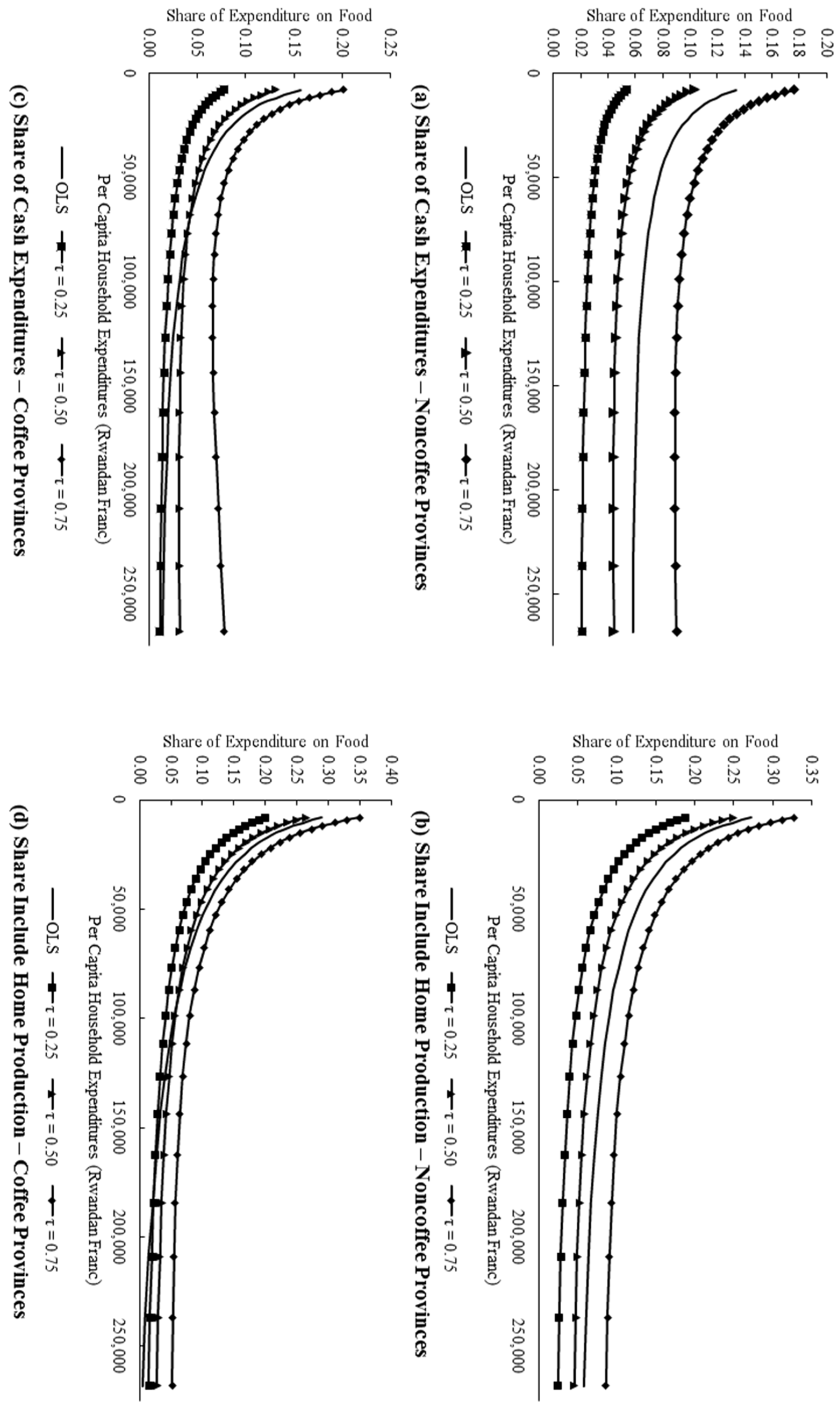
In
Figure 1a we present the estimated budget share for noncoffee provinces based on cash purchases while
Figure 1b presents the comparable budget shares including home production. The cash expenditures on food levels out after approximately 60,000 Rwanda Franc (RWF) in
Figure 1a. In addition, the quantile regression results increases slightly at around 250,000 RWF per capita. By comparison, the budget shares for food expenditures including home production presented in
Figure 1b declines relatively smoothly throughout the entire range. The results for coffee growing provinces are similar.
Figure 1c shows that share of cash income spent on food levels out at about 50,000 RWF. In addition, the minimum for expenditure share expenditure for food is reached at about 120,000 RWF. The expenditure shares on food then start to increase, rising from about 0.065 at 120,000 RWF to around 0.075 at 270,000 RWF. To compare the relative range of budget shares, the median budget share and relative inter-quartile range (e.g., the difference between 3rd quartile and the 2nd quartile divided by the median) for the graphs are presented in
Table 4. These results indicate that the more complete definition of expenditures yield more consistent Working’s relationships than the relationship using cash expenditures alone (e.g., the Working’s curves have smaller relative inter-quartile ranges).
We now focus on the more complete definition of household expenditures on food (
i.e., including home production as part of food production and adding the value of home production to household expenditures) and examine the implied difference in the income elasticity of food to address the question raised by the Minister of Agriculture and Animal Resources in Rwanda. Following the intuition from Kumar, Holla, and Guha [
4] and Theil, Chung, and Seale [
5] less food secure households have high income elasticities of demand for food (
i.e., a larger portion of the marginal income is dedicated to the purchase of food). The results in
Table 5 indicate that for the poorest households (
i.e., those households at the 1st quartile of income), the income elasticities are fairly similar.
Like the statistical results for the regression coefficients presented in
Table 1, the income elasticities for food are statistically significant at any conventional level of confidence. These results implicitly compare the estimated elasticity with zero (
i.e.,
). A more important question is whether the elasticities are the same. For example, a “paired
” test for the equivalence between the elasticity for the 1st quartile and the 3rd quartile would be
. Hence, the income elasticity for the 1st quartile is statistically different from the income elasticity for the 3rd quartile at any conventional level of confidence.
Table 6 and
Table 7 present the results for a slightly more general form of this test. Specifically,
Table 6 presents the
statistics for an analysis of variance (ANOVA) test for the hypothesis that the income elasticity of the 1st quartile equals to the income elasticity for the 3rd quartile and the hypothesis that the income elasticity is the same for the 1st quartile, the median and the 3rd quartile. These tests are computed using the data from the bootstrapping procedure used to generate the standard errors for the estimators in
Table 1 and income elasticities in
Table 5. The results in
Table 6 indicate that all the income elasticities are different across quantiles.
Table 7 presents a slightly different hypothesis—that the income elasticities are the same for each income quartile across types of provinces. One hypothesis is that the income elasticity for noncoffee provinces equals the income elasticity for coffee provinces for households in the first income quantile.
Given that the income elasticities are statistically different, the next question is whether these differences are economically significant. Consider the results for
. Following the development of the Working’s model, these observations are the most food insecure households (
i.e., those households who spend the highest share of their income on food). Further focusing on the 1st Quartile of expenditures (e.g., the poorest of these households), the income elasticity is 0.5474 in the pooled results, 0.5923 for noncoffee provinces, and 0.5111 in coffee provinces. Intuitively, the households in the noncoffee growing provinces appear to be the most food insecure. We assume that a household with an annual expenditure per capita of 11,750 RWF (a somewhat round number approximately equal to the 1st Quartile). This household would spend 3374 RWF on food under the pooled estimates, 2338 RWF on food under the estimates for noncoffee growing provinces and 3714 RWF on food under the estimates for the coffee growing provinces. Hence, households in the coffee growing provinces spend more money on food and thus appear more food secure. However, if household income was to increase by five percent (e.g., 587.50 RWF) the pooled expenditure on food would increase by 322 RWF, the expenditures on food for noncoffee producing provinces would increase by 348 RWF, and the expenditures on food for coffee growing provinces would increase by 300 RWF. Essentially, the Working’s curve for coffee growing provinces is steeper for coffee growing provinces than for noncoffee growing provinces (which is reasonable comparing
Figure 1b with
Figure 1d). So what does this mean? At one level, the results are consistent with Dr. Gerardine Muskeshimana’s contention. The results suggest that the most food insecure households in coffee growing regions buy less food with an increase in income than other food insecure households in Rwanda. However, this result hides the finding that these households already spend more for food (e.g., 3714 RWF for food insecure households in coffee regions compared with 2338 RWF in other areas).
4. Conclusions
Feed the Future is the major U.S. initiative to reduce poverty and end hunger worldwide. One of the major pathways for this initiative spearheaded by the United States Agency for International Development involves improving the returns to smallholder agriculture in 19 Feed the Future countries. In one of these countries (Rwanda), several programs have attempted to increase the returns to smallholders by improving the market channel for coffee. These efforts have been successful, increasing household income and reducing the incidence of poverty in provinces which produce coffee as a major cash crop. However, several have question whether these gains have actually reduced food security in these regions. Specifically, stunting and wasting remains a significant concern in these regions. In order to provide some insights into this question, this study compares the impact of additional income on food consumption between noncoffee producing and coffee producing provinces in Rwanda by applying quantile regression to a Working’s formulation of food demand.
The empirical results imply that the quantity of food purchased for each additional Franc is different for noncoffee and coffee producing provinces. While this result appears to support the contention that programs did not have the desired effect on food security, the direction of the effect shows the reverse is actually true. Households in coffee producing provinces actually spend more on food than households in other provinces when home production is included in the analysis. However, the results indicate that households in coffee producing provinces spend a smaller share of each additional Franc on food than do households in other provinces.
Additional work is required to flush out the effect of improving returns to smallholders on food security. Specifically, our linkage between food security and returns to smallholders is weak. Basically, we test the implications for the general conjecture that food security is improved when more food is purchased by the household. One possibility would be to gather data on stunting and wasting by district (each province in Rwanda contains several districts). The model estimated in this study could then be used to test the hypothesis that increased household expenditures on food reduces the probability of stunting.
Econometrically the significance of the results reported in this study are primarily the result of a fairly large sample (
i.e., 14,308 households). While standard bootstrapping results are typically fairly robust, one alternative would be to test the level of significance for the sample estimates and elasticities using a “wild bootstrapping” procedure [
10].


