Article

A Method for Measuring Treatment Effects on the Treated without Randomization

1
Federal Reserve Board (Retired), 6333 Brocketts Crossing, Kingstowne, VA 22315, USA
2
Leicester University, Room Astley Clarke 116, University Road, Leicester LEI 7RH, UK
3
Bank of Greece, 21 El. Venizelos Ave., 10250 Athens, Greece
4
Monetary Policy Council, Bank of Greece, 21 El. Venizelos Ave., 10250 Athens, Greece
5
Department of Mathematics and Statistics (Retired), The American University, Washington, DC 20016, USA
6
Economic Research Department, Bank of Greece, 21 El. Venizelos Ave., 10250 Athens, Greece
7
Department of Economics, New York University, 44 West Fourth Street, 7–90 New York, NY 10012, USA
8
Department of Mathematics (Retired), Temple University, Philadelphia, PA 19122, USA
*
Author to whom correspondence should be addressed.
Econometrics 2016, 4(2), 19; https://doi.org/10.3390/econometrics4020019
Submission received: 13 July 2015 / Revised: 22 February 2016 / Accepted: 9 March 2016 / Published: 25 March 2016
(This article belongs to the Special Issue Recent Developments of Financial Econometrics)

Abstract

:
This paper contributes to the literature on the estimation of causal effects by providing an analytical formula for individual specific treatment effects and an empirical methodology that allows us to estimate these effects. We derive the formula from a general model with minimal restrictions, unknown functional form and true unobserved variables such that it is a credible model of the underlying real world relationship. Subsequently, we manipulate the model in order to put it in an estimable form. In contrast to other empirical methodologies, which derive average treatment effects, we derive an analytical formula that provides estimates of the treatment effects on each treated individual. We also provide an empirical example that illustrates our methodology.

1. Introduction

Previous studies have dealt with the issue of estimating the average treatment effect on the treated (ATET) or the treatment effects averaged over the entire population (ATE). 1 These studies have typically relied on the estimation of average treatment effects; random assignment to treatment aims to ensure that individuals (or units) assigned to the treatment and individuals assigned to control are identical; the average outcome among the control individuals serves as the counterfactual for the average outcome among the treated individuals. The difference between those two averages is an estimate of the central tendency of the distribution of unobservable individual-level treatment effects. 2
Estimation of treatment effects is challenging when the treatment assignment is not completely random. In this paper, we provide a method that does not require either completely random assignment or data on pairs of individuals matched by some specific criterion—one subjected to control and the other subjected to the treatment. 3 Our model has unique coefficients and error terms and guards against incorrect functional forms. 4 We provide a precise specification for the treatment effect under the condition that individuals are self-selected into treatment. In deriving this specification, we use the following definition of the treatment effect: the effect of a treatment on a treated individual minus the outcome that would have been observed had the same individual not been treated (the counterfactual). 5 Thus, in contrast to previous studies, which deal with average treatment effects, our definition is individual specific. There are practical difficulties in empirically implementing our definition. In what follows, we describe these difficulties and provide solutions.
An intuitive explanation of the contribution of this paper is as follows. In a randomized trial, it is relatively easy to calculate the effect of a given treatment. This can be done simply by estimating a standard model with a dummy variable for the treatment: since we know that the treatment is random, it can be treated as exogenous. However, in a real-world situation without randomization, it is extremely unlikely that the treatment can be assumed to be exogenous. Consider the case of a new cancer treatment. Clearly, the treatment would only be given to patients who are severely ill and likely to die. The treatment is not random and, therefore, simply adding a dummy for treated individuals is likely to be highly misleading and may even lead us to conclude that the treatment causes the patients to die from the illness. The empirical literature has attempted to deal with this problem by using instrumental variables (in a variety of ways). However, the difficulties of weak or irrelevant instruments are well-known. 6 This paper offers a new approach to this problem, based on coefficients that vary. Our approach avoids both the misspecification caused by incorrect functional forms, and provides coefficients that absorb omitted regressors, measurement errors and endogeneity. These varying coefficients may then be decomposed to obtain an estimate of the true underlying treatment effect.
The remainder of the paper consists of three sections. Section 2 consists of several parts. It begins by reviewing the concepts needed to define the causal effect of a treatment on a treated individual. The section then develops two models that contain what we characterize as “unique coefficients and error terms”—one model for the causal effects attributable to the treatment and the other model for the unknown values of what “response” the individuals who participated in a treatment would have had they not been treated. In this connection, we provide both a formal derivation and an intuitive account of our theoretical derivation. Finally, the section discusses the issue of identification, presents a possible method of estimation of these models, and derives the predictions of the treatment effects. Section 3 provides an empirical example to illustrate our method. Section 4 concludes.

2. Modeling the Effect of a Treatment on the Treated in Non-Experimental Situations

2.1. Preparations

2.1.1. Notation

Let i index treated individuals and let i ( i) index untreated individuals. 7 The number of treated individuals is denoted by n 1 and that of untreated individuals is denoted by n 2 . Let n 1 + n 2 = n , the size of a sample of both treated and untreated individuals. Both n 1 and n 2 are known. We assume that the individual response to treatment is heterogeneous. The dummy variable C is defined to take the value 0 for untreated individual i and to take the value 1 for treated individual i. For untreated individual i , ( y i * | C i = 0) = y 0 i * is the unobserved true value of the observed outcome ( y 0 i ) of no treatment; y 0 i * plus measurement error ( u 0 i * ) is the observed value, y 0 i . For treated individual i, ( y i * | C i = 1) = y 1 i * , y 1 i = y 1 i * + u 1 i * where y 1 i * is the (unobserved) true value of the observed outcome ( y 1 i ) of a treatment and u 1 i * is measurement error.

2.1.2. Potential Outcome Notation

Pratt and Schlaifer [7] (pp. 28 and 35) used Neyman’s potential-outcome notation to state causal laws. 8 Potential outcomes can be recognized through the subscripts that are attached to counterfactual events (see Pearl [10] (p. 3)). Symbolically, potential outcomes are denoted by Y x i , which shows the value that outcome Y would take for individual i had the treatment X been at level x.

2.1.3. Counterfactuals

The symbol y 1 i * denotes a value of what the outcome would have been had individual i been treated. The symbol y 0 i * denotes a value of what the outcome would have been had individual i not been treated. The variables y 1 i * and y 0 i * are the unobserved counterfactuals implicit in the true values y 0 i * and y 1 i * , respectively. Both the values of y 0 i (the effects of no treatment on the untreated individuals) and y 1 i (the effect of treatment on the treated individual) are observed but they both cannot be observed for the same individual since y 1 i refers to a treated individual and y 0 i refers to an untreated individual.

2.1.4. Treatment Effects in a Pure Sense

In the treatment effect on the untreated, defined by y 1 i * y 0 i * , y 0 i * is the unobserved true value; it differs from the observed value y 0 i by a measurement error, and the counterfactual y 1 i * has no observations for all untreated individuals i = 1, …, n 2 . In the treatment effect on the treated, defined by y 1 i * y 0 i * , y 1 i * is the unobserved true value, it differs from the observed value y 1 i by a measurement error, and the counterfactual y 0 i * has no observations for all treated individuals i = 1, …, n 1 .

2.1.5. The Purpose of the Paper

In Section 2.2 below, we derive the models of y 1 i * and y 0 i * that give the predictions of their dependent variables, respectively. Following Greene [1] (p. 888), we believe that an accurate estimate of the treatment effect y 1 i * y 0 i * on the treated is more useful than an accurate estimate of the treatment effect y 1 i * y 0 i * on the untreated. 9 That is, it is more natural to ask, what is the treatment effect on a treated individual, rather than ask, what would have been the treatment effect on an untreated individual? 10 In the following subsections, we derive an analytical formula for y 1 i * y 0 i * .

2.1.6. What is Causality?

Previous researchers have set-forth various definitions of causality. In this section, we show how our specification of a treatment effect relates to several of those definitions. Our aim here is not to provide a comprehensive discussion of the causality literature.
  • First, Basmann [11] (p. 99) revealed that common to all of the generally accepted meanings of “causality” is the notion that causality is a property of the real world and is not an algebraic property of the mathematical representations of parts of the real world. An insight that follows from this notion is that real-world relationships do not contain specification errors. This insight suggests that statistical causation requires deriving estimates within an environment free of specification errors. With regard to the definition of treatment effects, the notion requires that, to measure causal effects, we should calculate the difference between the real-world relations for the outcome of a treatment and the potential outcome of no treatment on the same individual. In what follows, we empirically implement this definition.
  • Second, to show statistical causation, Skyrms [12] proved that positive statistical relevance needs to continue to hold when all relevant pre-existing conditions are controlled for. 11 Intuitively, the relevant pre-existing conditions can be thought of as all the factors that might affect a relationship but which cannot be captured (for example, omitted variables). For example, the typical empirical counterpart to household consumption function is derived from a utility function. We do not know how to measure the utility function, but it governs the actual structure of the consumption function. We control for such pre-existing conditions.
To be specific, we follow generally accepted meanings of causality. We follow Basmann’s clarification that causal relations should be free of specification errors and Skyrms’ definition of statistical causation which stresses the need to control for pre-existing conditions. To account for Skyrms’ [12] (p. 59) and Basmann’s [11] (p. 99) insights on these issues, we derive real-world relationships—that is, relationships free of all specification errors—under the insight that causality is a property of the real world. Skyrms’ insight leads to the conclusion that all irrelevant variables need to be eliminated from a relationship. To find such a relationship, we start with a general nonlinear mathematical model with unknown functional form, in which the dependent variable satisfies the normalization rule (that the coefficient of the dependent variable equals unity), and the arguments of the mathematical function include all the determinants of the dependent variable and all the relevant pre-existing conditions. We express this model as linear in variables and nonlinear in coefficients. These coefficients are the partial derivatives of the function with respect to its arguments. It can be verified that this linear-in-variables and nonlinear-in-coefficients model has the correct functional form. These partial derivatives keep the values of all relevant pre-existing conditions constant. Specifically, we: (i) follow Basmann’s [11] notion of causality because it is not restrictive (it necessitates the absence of specification errors); (ii) follow Skyrms’ [12] elucidation of statistical causation; (iii) work with the partial derivatives of some deterministic real-world (i.e., misspecification-free) relationships to control for all relevant pre-existing conditions; (iv) use the frequentist probability to measure causal effects; and (v) work with the misspecification-free models of y 1 i * and y 0 i * to evaluate y 1 i * y 0 i * . 12
Finally, in articulating a definition of causality, we also take account of the insights provided by Zellner [13] and Pratt and Schlaifer [7]. Zellner adopted Feigl’s definition according to which causality is “predictability according to a law or set of laws.” Pratt and Schlaifer defined a law with factors and concomitants and provided the conditions under which the laws can be observed in data. 13 In what follows, we develop both a set of laws and the necessary additional variables—which we call coefficient drivers—needed to empirically implement the laws. 14

2.2. The Correctly Specified (or Misspecification-Free) Models of y 1 i * , y 1 i , and y 0 i *

2.2.1. Mathematical Functions

To generate the predictions for y 1 i * , y 1 i , and y 0 i * , we begin with their real-world relationships expressed in terms of the following mathematical equations.
y c η *   =   f c η ( x c η 1 * , ... , x c η , L c η * )
where c ( 0 , 1 ) , η ( i , i ) . Since Equation (1) is a mathematical equation, it does not contain an error term.
Henceforth, f c η ( x c η 1 * , ... , x c η , L c η * ) will be written more compactly as f c η ( . ) . The precise functional form of this function is unknown; x c η 1 * , ... , x c η , L c η * are the arguments of f c η ( . ) . These arguments are of three types: (i) observed and (ii) unobserved determinants of y c η * and (iii) all relevant pre-existing conditions; the number L c η of all these arguments is an unknown integer dependent on c and η , since the number of the arguments of types (ii) and (iii) is unknown. Why include type (iii) arguments in f c η ( . ) ? The answer is provided by Skyrms’ [12] (p. 59) definition that mathematical causation is positive mathematical relevance which does not disappear when we control for all relevant pre-existing conditions. To control for these conditions, we first include them directly into f c η ( . ) as its arguments and take the partial derivatives of f c η ( . ) with respect to its type (i) and type (ii) arguments that keep the values of these conditions constant. In this way, we control for all relevant pre-existing conditions.
Next, we use these partial derivatives as the coefficients of Equation (2) below. There are no relevant arguments excluded from f c η ( . ) . Therefore, there is no need to introduce an error term into f c η ( . ) to represent nonexistent omitted variables. Alternatively stated, all the variables constituting the econometrician’s error term are treated as the arguments of f c η ( . ) . This is done to avoid all incorrect functional forms of f c η ( . ) . The symbols β 1 , β 2 , ... , β K may be used to denote the constant features of f c η ( . ) . We do not treat any features of f c η ( . ) as constant parameters because, as Goldberger [15] pointed out in the context of the Rotterdam school demand models, the treatment of any particular features of f c η ( . ) as constants may be questioned.

2.2.2. Minimally Restricted Relations

The only restriction that we have imposed on Equation (1) is the normalization rule that the coefficient of y c η * is equal to unity.

2.2.3. Available Data for Estimation of (1)

We assume that L 1 i > K + 1 < L 0 i , K + 1 < n 1 and n 2 . Data on x c η 1 * , …, x c η K * are available. These data may contain measurement errors, i.e., x c η 1 = x c η 1 * + ν c η 1 * , …, x c η K = x c η K * + ν c η K * , where the variables without an asterisk are observable, the variables with an asterisk are true and unobservable, and the ν * ’s are measurement errors. 15 We call x c η 1 , …, x c η K “the included arguments of f c η ( . ) ”. 16 Also available are data on y 0 i for n 2 untreated individuals and on y 1 i for n 1 treated individuals. For treated individuals with c = 1, y 1 i is observed with measurement error and a non-constant proxy, denoted by x 1 i , K + 1 * , for the treatment variable is used as an additional included argument of f 1 i ( . ) . 17 Let x 1 i , K + 1 = x 1 i , K + 1 * + ν 1 i , K + 1 * where the variable without an asterisk is observable, the variable with an asterisk is true and unobservable, and the ν 1 i , K + 1 * ’s are measurement errors. No data on x c η , K + 2 * , …, x c η , L c η * are available and hence they can only be treated as omitted arguments. 18,19

2.2.4. Correctly Specified Models for y 1 i and the Counterfactual y 0 i * for the Same Individual i

Without misspecifying its functional form, (1) can be expressed as
y c η *   =   α c η 0 * + j = 1 K x c η j * α c η j * + x c η , K + 1 * α c η , K + 1 * + g = K + 2 L c η x c η g * α c η g *
where for = 1, …, L c η , the coefficient of x c η * is equal to y c η * / x c η * unless x c η * is discrete, in which case this partial derivative is approximated by Δ y c η * / Δ x c η * with the right sign where Δ y c η * and Δ x c η * are small differences in the values of y c η * and x c η * , respectively, and the intercept α c η 0 * is equal to y c η * j = 1 L c η x c η j * α c η j * . This α c η 0 * is the error of approximation that results from approximating f c η ( . ) by j = 1 L c η x c η j * α c η j * . Equation (2) is obtained from y c η * = f c η ( x c η 1 * , ... , x c η , L c η * ) j = 1 L c η x c η j * α c η j * + j = 1 L c η x c η j * α c η j * where α c η 0 * = f c η ( x c η 1 * , ... , x c η , L c η * ) j = 1 L c η x c η j * α c η j * . From this it follows that Equation (2) without α c η 0 * will have the correct functional form when α c η 0 * = 0. For our further analysis of (1), it is convenient to express it in the form of Model (2) that is linear in variables but nonlinear in coefficients. We avoid the use of any incorrect functional form of (1) by defining the coefficients of (2) as the partial derivatives of f c η ( . ) with respect to its arguments. The coefficient α c η , K + 1 * is zero for untreated individuals. It follows that the problem of estimating f c η ( . ) with unknown functional form is solved by changing it to that of estimating certain partial derivatives of f c η ( . ) .
Equation (2) is linear if its coefficients are constant and nonlinear otherwise. How do we ensure that α c η , K + 1 * is the causal effect of x c η , K + 1 * on y c η * holding the values of all arguments of f c η ( . ) other than x c η , K + 1 * constant? This constancy condition is true because α c η , K + 1 * is the partial derivative of y c η * with respect to x c η , K + 1 * . In the definition of this partial derivative, not only the values of all determinants of y c η * other than x c η , K + 1 * but also the values of all relevant pre-existing conditions are held constant. This is a standard way to eliminate the false relationship between y c η * and any of its determinants (see Skyrms [12] (p. 59)). For example, suppose that the relationship of y c η * to x c η 1 * is false. Then, the partial derivative of y c η * with respect to x c η 1 * is zero because the values of all relevant pre-existing conditions are held constant. Also, we do not impose on (1) any restriction that makes it lose the causal invariance property of real-world relations described in Section 2. These precautions are taken to ensure that the partial derivatives used as the coefficients of (2) are the truths, meaning the properties of the real-world relationship in (1).
Treated individual i: We now apply the specification in (2) to the particular group of treated individuals. From (2) it follows that
y 1 i *   =   α 1 i 0 * + j = 1 K x 1 i j * α 1 i j * + x 1 i , K + 1 * α 1 i , K + 1 * + g = K + 2 L 1 i x 1 i g * α 1 i g *
where y 1 i = y 1 i * + u 1 i * , y 1 i is observed, y 1 i * is the unobserved true value, u 1 i * is measurement error, the treatment regressor x 1 i , K + 1 * is added to the list x 1 i 1 * , ... , x 1 i , K * but not to the list x 1 i , K + 2 * , ... , x 1 i , L 1 i * , since Equation (3) is for a treated individual. The coefficients of (3) are the truths about the real-world relationship in (1). Note that the set of variables denoted by g = k + 2 L 1 i x 1 i g * a 1 i g * are unobserved and need to be eliminated. To eliminate those unobserved variables, we regress each of these variables on all observed variables as follows.
x 1 i g * = λ 1 i g 0 * + j = 1 K + 1 x 1 i j * λ 1 i g j * ( =   K + 2 , , L 1 i )
where λ 1 i g j * = x 1 i g * / x 1 i j * if x 1 i j * is continuous and = Δ x 1 i g * / Δ x 1 i j * with the right sign otherwise and λ 1 i g 0 * = x 1 i g * j = 1 K + 1 x 1 i j * λ 1 i g j * . This definition makes Equation (4) exact.
Model of y 1 i * with unique coefficients and error term: Substituting the right-hand side of Equation (4) for x 1 i g * in (3) gives
y 1 i * = α 1 i 0 * + g = K + 2 L 1 i λ 1 i g 0 * α 1 i g * + j = 1 K + 1 x 1 i j * ( α 1 i j * + g = K + 2 L 1 i λ 1 i g j * α 1 i g * )
where g = K + 2 L 1 i λ 1 i g 0 * α 1 i g * and ( α 1 i j * + g = K + 2 L 1 i λ 1 i g j * α 1 i g * ) are the unique error term and coefficients, respectively (see Swamy et al. [4] (p. 199)). The formula g = K + 2 L 1 i λ 1 i g j * α 1 i g * measures omitted-regressors bias of the coefficient of x 1 i j * . For j = 1,…, K + 1, the α 1 i j * ’s are the partial derivatives of (1) with c = 1 and η = i.
Equation (1) for c = 1 and η = i and (5) are the two forms of the same real-world relationship in (1).
Recall, the variables y 1 i * and x 1 i j * , j = 1, …, K + 1, in Equation (5) are the true values and are not the observed values. To express (5) in terms of the observed values, we insert measurement errors at the appropriate places in (5). Doing so gives
y 1 i   =   γ 1 i 0   +   j = 1 K + 1 x 1 i j γ 1 i j
where
γ 1 i 0   =   α 1 i 0 *   +   g = K + 2 L 1 i λ 1 i g 0 * α 1 i g *   +   u 1 i * x S 2 v 1 i j * ( α 1 i j * + g = K + 2 L 1 i λ 1 i g j * α 1 i g * )
γ 1 i j = ( 1 v 1 i j * x 1 i j ) ( α 1 i j * + g = K + 2 L 1 i λ 1 i g j * α 1 i g * )  if  x S 1
= ( α 1 i j * + g = K + 2 L 1 i λ 1 i g j * α 1 i g * )  if  x S 2
S 1 is the set of all continuous regressors of Equation (6) and S 2 is the set of all regressors of (6) that take the value zero with positive probability. In Equations (7) and (8), − x S 2 v 1 i j * ( α 1 i j * + g = K + 2 L 1 i λ 1 i g j * α 1 i g * ) and ( v 1 i j * x 1 i j ) ( α 1 i j * + g = K + 2 L 1 i λ 1 i g j * α 1 i g * ) are the measurement-error biases of γ 1 i j if x S 2 and x S 1 , respectively. 20 These measurement-error biases are not unique.
What would have been the outcome, denoted by y 0 i * , had the ith individual not been treated? We determine this outcome by setting the treatment x 1 i , K + 1 * equal to zero in (3). Doing so gives
y 0 i * = y 1 i x 1 i , K + 1 * α 1 i , K + 1 * u 1 i * = α 1 i 0 * + j = 1 K x 1 i j * α 1 i j * + g = K + 2 L 1 i x 1 i g * α 1 i g *
where y 0 i * = y 1 i x 1 i , K + 1 * α 1 i , K + 1 * u 1 i * = y 0 i u 0 i * , y 0 i * is the unobserved true value, u 0 i * is measurement error, and α 1 i 0 * = y 0 i * = 1 L 0 i x 1 i * α 1 i * + x 1 i , K + 1 * α 1 i , K + 1 * .
The treatment causal effect (TCE) on the ith treated individual
y 1 i * y 0 i * = ( y 1 i u 1 i * ) ( y 0 i u 0 i * ) = { ( α 1 i 0 * + j = 1 K x 1 i j * α 1 i j * + x 1 i , K + 1 * α 1 i , K + 1 * + g = K + 2 L 1 i x 1 i g * α 1 i g * + u 1 i * ) u 1 i * } { ( α 1 i 0 * + j = 1 K x 1 i j * α 1 i j * + g = K + 2 L 1 i x 1 i g * α 1 i g * + u 0 i * ) u 0 i * } = x 1 i , K + 1 * α 1 i , K + 1 *
Thus, to derive the TCE, Equations (3) and (10) enable us to derive the TCE in Equation (11). However, Equation (11) is an analytical equation. To estimate the TCE in Equation (11), we need to complement Equation (6) with additional equations.

2.2.5. In What Way Are the Coefficients and Error Term of (5) Unique?

The arguments, x 1 i 1 * , ... , x 1 i , K + 1 * , included in both (3) and (5) are called “the included regressors” and the arguments x 1 i , K + 2 * , ... , x 1 i , L 1 i * included in (3) but not in (5) are called “omitted regressors.” These regressors are not unique. 21 The coefficients and error term of (5) have the correct functional forms and, as a result, are unique in the sense that they are invariant under the addition and subtraction of the coefficient of any omitted regressor times any included regressor on the right-hand side of Equation (3). 22 It can be shown that the error term of (5) is the unique function g = K + 2 L 1 i λ 1 i g 0 * α 1 i g * (with the correct functional form) of the “sufficient sets” ( λ 1 i g 0 * , g = K + 2, … , L 1 i ) of omitted regressors, a concept given by Pratt and Schlaifer [7] (p. 34). The uniqueness of its coefficients and error term means that (5) possesses the causal invariance property.

2.2.6. What Specification Errors is the TCE Free from?

(i) We have ensured that the unknown functional forms of (3) and (4) did not become the source of specification errors. (ii) By ensuring that the coefficients and error term of (5) are unique, the specification errors resulting from non-unique coefficients and error terms are not allowed to occur; (iii) Pratt and Schlaifer [7] (p. 34) pointed out that the requirement that the included regressors be independent of the excluded regressors themselves is “meaningless”. The specification error introduced by making this meaningless assumption is avoided by taking a unique function of certain “sufficient sets” of omitted regressors as the error term of (5); (iv) The specification error of ignoring measurement errors when they are present is avoided by placing them at the appropriate places in (5) to obtain Equation (6). The TCE in (11) is derived from Equations (3) and (10) which are free of specification-errors (i)–(iv). It should be noted that when we state that (3), (6), (10) and (11) are free of specification errors, we mean that they are free of specification-errors (i)–(iv). Using (1)–(5), we have derived a real-world relationship in (6) that is free of specification-errors (i)–(iv). Thus, our approach affirms that any relationship suffering from any one of these specification errors is definitely not a real-world relationship.

2.2.7. Specification Errors and Omitted-Regressor Biases

It is useful here to refer to a highly-influential paper by Yatchew and Griliches (YG) [17]. Those authors considered a simple binary choice model with any two regressors (X1 and X2) with nonunique coefficients and an error term and omitted from it one (X2) of its two regressors. YG showed that even if the omitted regressor is uncorrelated with the included regressor, the coefficient on the included regressor will be inconsistent. In addition, they showed that if the disturbances in the underlying regression are heteroscedastic, then the maximum likelihood estimators that assume homoscedasticity are inconsistent and the covariance matrix is inappropriate. What is important here is that not only the omission of a regressor from the YG model, but also the omitted regressors implicit in the YG’s mean-zero error term introduce biases from omitted variables. Furthermore, the YG results are subject to the four specification errors discussed in the previous section. As noted, our approach, using Equations (1)–(6), avoids these specification errors.

2.2.8. The Available Data Are Not Adequate to Estimate TCE

There are practical difficulties in estimating the TCE, x 1 i , K + 1 * α 1 i , K + 1 * , because the partial derivative α 1 i , K + 1 * in (6) is corrupted by omitted-regressor and measurement-error biases. These omitted-regressor biases arise as a direct consequence of using the equations in (4) to remove x 1 i g * , g = K + 2, …, L 1 i , from (3), and measurement-error biases arise as a direct consequence of measurement errors in x c η 1 = x c η 1 * + ν c η 1 * , …, x c η , K + 1 = x c η , K + 1 * + ν c η , K + 1 * . Unless these biases are eliminated from γ 1 i , K + 1 we cannot obtain consistent estimate of α 1 i , K + 1 * . We will show below what additional data are needed for this removal.

2.3. Variable Coefficient Regression

The model for Y x i is the same as Model (6) for y 1 i . Rewrite this model as
Y x i = y 1 i = x 1 i   γ 1 i ( i = 1 ,   ,   n 1 )
where x 1 i = ( 1 , x 1 i 1 , ... , x 1 i , K + 1 ) is the (K + 2) × 1 vector of regressors, γ 1 i = ( γ 1 i 0 , γ 1 i 1 , ... , γ 1 i . K + 1 ) is the (K + 2) × 1 vector of coefficients. We characterize this model as “the correctly specified model” because the model is derived from the real-world relationship in (1) without making any specification error. Similarly, Equation (10) is the correctly specified model of the counterfactual ( y 0 i * ). In Equation (11), it is shown that TCE = y 1 i * y 0 i * = x 1 i , K + 1 * α 1 i , K + 1 * . To estimate this TCE, we use (8) or (9) which shows that α 1 i , K + 1 * = γ 1 i . K + 1 —its omitted-regressor and measurement-error biases. We first estimate γ 1 i . K + 1 and decompose it into an estimate of α 1 i , K + 1 * and an estimate of γ 1 i . K + 1 ’s omitted-regressor and measurement-error biases.

2.3.1. Parameterization of the Variable Coefficient Regression

Equation (12) is estimated subject to the restrictions Equations (7)–(9) imposed on its coefficients. To make such estimation feasible, we assume that for j = 0, 1, …, K + 1,
γ 1 i j = π 1 j 0 + h = 1 p z 1 i h π 1 j h + ε 1 i j
where the z 1 i h ’s are observable and are called “the coefficient drivers”, some of which may be common among different coefficients of (12), and the π s are unknown fixed parameters. 23,24 The error term ε 1 i j is treated as a random variable. 25
A key justification for Equation (13) is that it facilitates separate estimation of each component of the coefficients of (12), as will be obvious from Equation (20) below. For each j, given the proportion of measurement error v 1 i j * x 1 i j in (8), the coefficient drivers in (13) should split into two sets so that one set explains most of variation in the bias-free component ( α 1 i j * ) and the other set explains most of variation in omitted-regressor bias component ( g = K + 2 L 1 i λ 1 i g j * α 1 i g * ) in (8). These sets may or may not be non-overlapping. We will make use of these conditions in Equation (20) below.
Note that if (1) is nonlinear, then the α 1 i j * ’s are functionally dependent on the x 1 i j * ’s and x 1 i g * ’s including x 1 i , K + 1 * . This introduces correlations between x 1 i and γ 1 i . In the presence of these correlations, we proceed as follows:
Admissibility condition: The vector Z 1 i = ( Z 1 i 0 , Z 1 i 1 , ... , Z 1 i p ) in Equation (13) is an admissible vector of coefficient drivers if, given Z 1 i , the value that the coefficient vector of (12) would take in unit i, had X 1 i = ( X 1 i 1 , ... , X 1 i , K + 1 ) been x 1 i = ( x 1 i 1 , ... , x 1 i K + 1 ) is independent of X 1 i for all i. 26
It is shown in (8) or (9) that the first component of the coefficient of each nonconstant regressor in (12) keeps the values of all relevant pre-existing conditions constant. Skyrms [12] (p. 59) argued that this “comes to much the same as identifying the appropriate partition, … , ((or σ -field)) which together with … (or value of the causal variable) ( x 1 i , K + 1 ) determines the chance of the effect.” We show below that this partition is less adequate than the partition implied by Equation (13) for our purposes.
It should be understood that the coefficient drivers in (13) are not the same as the regressors in (12). The coefficient drivers explain variations in the components of the coefficients of (12), whereas the regressors of (12) in conjunction with its coefficients explain variation in the dependent variable y 1 i . We discuss the selection of coefficient drivers below.
We use the following matrix notation: z 1 i = (1, z 1 i 1 , ... , z 1 i p )′ is ( p + 1 ) × 1 , π 1 j = ( π 1 j 0 , π 1 j 1 , ... , π 1 j p ) is 1 × ( p + 1 ) , Π 1 is a (K + 2) × ( p + 1) matrix having π 1 j as its jth row, and ε 1 i = ( ε 1 i 0 , ... , ε 1 i K + 1 ) is the ( K + 2 ) × 1 error vector, and γ 1 i j = π 1 j z 1 i + ε 1 i j is a scalar.
Substituting the right-hand side expressions of the (K + 2) equations in (13) for the (K + 2) coefficients in (12), respectively, gives the result which, in matrix form, can be written as 27
y 1 i = x 1 i Π 1 z 1 i + x 1 i ε 1 i ( i = 1 ,   ,   n 1 )   28
Suppose that the admissibility condition for the coefficient drivers given in this section is not sufficient for the existence of the conditional expectation E( y 1 i | x 1 i , z 1 i ). Then, we make
Assumption I
For all i, let g ( x 1 i , z 1 i ) be a Borel function of ( x 1 i , z 1 i ) , E| y 1 i | < , and E| y 1 i g ( x 1 i , z 1 i ) | < .
Under this assumption, the conditional expectation
E ( y 1 i | x 1 i , z 1 i ) = x 1 i Π 1 z 1 i
exists (see Rao [18] (p. 97)).
Assumption II
For i = 1, …, n 1 , given z 1 i , ε 1 i is conditionally independent of x 1 i , and given z 1 i and x 1 i , the ε 1 i ’s are conditionally distributed with means zero and constant covariance matrix E ( ε 1 i ε 1 i | z 1 i , x 1 i ) = σ 1 ε 2 Δ 1 ε .
Cross-sectional data for treated individuals
y 1 i , x 1 i , and  z 1 i , i = 1 ,   ,   n 1
The number of observations in (16) is adequate to estimate all the unknown parameters of Equation (14) if n 1 (K + 2)(p + 1) + ( K + 2 ) ( K + 3 ) / 2 + 5 − r where r is the number of restrictions on the π s. With this condition, at least 4 degrees of freedom will remain unutilized after estimating all the unknown parameters of (14).

2.3.2. Identification of Model (14)

Let denote a Kronecker product and let vec(.) denote a column stack. Then, (K + 2) × ( p + 1) matrix Π 1 is identified if the matrix having ( z 1 i x 1 i ) as its ith row has full column rank. Even though the error vector ε 1 i is not identifiable, the inner product x 1 i ε 1 i is identifiable, since x 1 i ε 1 i = y 1 i − ( z 1 i x 1 i ) vec ( Π 1 ) . The variance-covariance matrix σ 1 ε 2 Δ 1 ε is consistently estimable from feasible best linear unbiased predictors of x 1 i ε 1 i . A necessary condition for the identifiability of both Π 1 and σ 1 ε 2 Δ 1 ε is that the information matrix for Model (14) is positive definite.

2.3.3. Identification of Model (12)

Because of the presence of more than one component in each coefficient of (6), we need the following identification condition: Model (12) is said to be identifiable on the basis of y 1 i , x 1 i and z 1 i , i = 1, …, n 1 , if the components of its coefficients are accurately estimable.

2.4. Estimation of Model (14) Under Assumptions I and II

Applying an iteratively rescaled generalized least squares (IRSGLS) method and the feasible best linear unbiased predictor to (14), we obtain the estimates of ( Π 1 , σ 1 ε 2 Δ 1 ε ) and the predictions of ε 1 i ’s. 29 Let these estimates and predictions be denoted by ( Π ^ 1 , σ ^ 1 ε 2 Δ ^ 1 ε ) and the ε ^ 1 i ’s, respectively. Inserting these into (13) gives the estimates of the coefficients of (12). Therefore, the estimated versions of (12) and (13) can be written as
y ^ 1 i = γ ^ 1 i 0 + j = 1 K + 1 x 1 i j γ ^ 1 i j
γ ^ 1 i j = π ^ 1 j 0 + h = 1 p z 1 i h π ^ 1 j h + ε ^ 1 i j
An iteratively rescaled generalized least squares method when applied to Equation (14) gives the estimates of π and ε in Equation (18) and these estimates, in turn, give the estimates of the coefficients of (17).

2.5. Estimation of a Component of a Coefficient of (12) by Decomposition

2.5.1. Estimation of Treatment Effects

In this section, we estimate the TCE, x 1 i , K + 1 * α 1 i , K + 1 * , derived in (11). If x 1 i , K + 1 is observed, then we use it in place of x 1 i , K + 1 * . We use (18) to estimate, α 1 i , K + 1 * , which is an unobserved bias-free component of γ 1 i , K + 1 , the coefficient of the treatment variable, x 1 i , K + 1 , in (17).
Theorem
In Model (6) which does not contain the specification errors (i)–(iv) discussed in Section 2.2.6, the coefficient, γ 1 i , K + 1 , on the continuous treatment variable x 1 i , K + 1 is equal to
( 1 D 1 i , K + 1 * ) A 1 i , K + 1 * + ( 1 D 1 i , K + 1 * ) B 1 i , K + 1 *
where D 1 i , K + 1 * = ( v 1 i , K + 1 * x 1 i , K + 1 ) = the proportion measurement error in the treatment variable, A 1 i , K + 1 * = α 1 i , K + 1 * = bias-free component, B 1 i , K + 1 * = g = K + 2 L 1 i λ 1 i g , K + 1 * α 1 i g * = omitted-regressor bias component, and (− D ^ 1 i , K + 1 * A ^ 1 i , K + 1 * - D ^ 1 i , K + 1 * B ^ 1 i , K + 1 * ) = measurement-error bias component of γ 1 i , K + 1 . It can be seen from (19) that bias-free component and bias components of γ 1 i , K + 1 are not additively separable.
Proof
See Equation (8) for the continuous x 1 i , K + 1 * treatment variable. Q.E.D.
The choice of regressors to be included in (12) is entirely dictated by the partial derivatives of (1) we want to learn. In this paper, we want to learn only about α 1 i , K + 1 * . Therefore, we reduce (12) to y 1 i = γ 1 i 0 + x 1 i 1 γ 1 i 1 and consider (13) only for γ 1 i 0 and γ 1 i 1 .
Selection of drivers: If in the real world a causal relationship exists that determines a particular variable—say, interest-rate spreads—then if one of the variables—say, x—in that relationship changes, the interest-rate spread will also change. This circumstance implies that the partial derivative of the interest-rate spread with respect to x is nonzero. Consequently, if we had a method of obtaining consistent estimates of this partial derivative, we would be able to infer that there is a real-world relationship between the interest-rate spread and variable x even though we may not know the exact functional form and all the variables that comprise the relationship. Moreover, our method of obtaining consistent estimates would apply if we allow for measurement error.
To implement a parametric method for estimating consistent estimates of the partial derivative in question, two assumptions are needed. First, we assume that the stochastic coefficients of the relationship we seek to uncover are themselves determined by a set of stochastic linear equations; the set of exogenous variables in these equations are what we have above called coefficient drivers. Second, we assume that some of these drivers are correlated with the misspecification in the model—that is the drivers “absorb” the specification errors—and some are correlated with the variation emanating from the (true) nonlinear form. With this assumption, we can simply remove the bias from the coefficients by removing the effect of the coefficient drivers that are correlated with the misspecification. For a valid driver, we need variables that are correlated with the misspecification.
The next step is the selection of the coefficient drivers in (13). The first point to understand is what constitutes a “good” driver set; this issue is discussed in detail in Hall Tavlas and Swamy [22]. The basic idea presented there is that the varying coefficient γ 1 i j will always capture the necessary variation in order to fully explain the dependent variable. This is because of the presence of the error term in the driver equation. However, to successfully decompose the coefficient into the bias free part and the biased part, the drivers must explain a large amount of the variation in the coefficient. Therefore, the first requirement for a good driver set is that it explains most of the variation in the coefficient. This result, however, can always be achieved by simply including a large number of drivers in the equation. Yet, such a procedure would not allow for a useful decomposition. Consequently, the second requirement is that the drivers must be individually relevant in explaining the movement in the coefficient—that is, they must be statistically significant. There are several approaches that can be used for this purpose. We would suggest starting from the relevant theory in terms of selecting a large set of possible drivers by asking what variables might capture omitted variables measurement errors and non-linearities. Once a driver set is selected, there are then several options to select a suitable sub-set for actual use. This procedure amounts to using objective criteria to select relevant drivers. The procedure could include the following elements:
  • Adopt a dynamic modelling approach of general to specific, nesting down from the large set of drivers to a parsimonious, smaller set.
  • Adopt information criteria such as AIC, SBC, and pick the driver set which minimizes the criteria.
  • Hall, Tavlas, Swamy and Tsionas [23] suggest a version of the stochastic search variable selection (SSVS) approach of George, Sun and Ni [24], which performs well in Monte Carlo experiments. (See also Jochmann, Koop and Strachan [25].)
The model can then be used in standard ways to either test an individual theory or to test between theories.
Equations (18) and (19) imply that
γ 1 i , K + 1 = π ^ 1 , K + 1 , 0 + h = 1 p z 1 i h π ^ 1 , K + 1 , h + ε ^ 1 i , K + 1 = [ ( 1 D ^ 1 i , K + 1 * ) A ^ 1 i , K + 1 * + ( 1 D ^ 1 i , K + 1 * ) B 1 i , K + 1 * ]
This equation reconciles the discrepancies between the functional forms of the quantities on either side of its second equality sign. We have the values of all the terms on the left-hand side of the second equality sign in Equation (20). From these values, it can be shown that A ^ 1 i , K + 1 * and B ^ 1 i , K + 1 * are equal to ( 1 D 1 i , K + 1 * ) 1 × ( π ^ 1 , K + 1 , 0 + h G 1 z 1 i h π ^ 1 , K + 1 , h ) and ( 1 D 1 i , K + 1 * ) 1 ( h G 2 z 1 i h π ^ 1 , K + 1 , h + ε ^ 1 i j ) for some groupings G 1 and G 2 of the coefficient drivers, respectively. If these equalities hold, then we will not be making specification errors (i)–(iv).
Although we do not have the values of D ^ 1 i , K + 1 * and G 1 , we can only make some reasonable assumptions about them.
Assumption III
For all i: (i) The measurement error ν 1 i , K + 1 * forms a negligible proportion of x 1 i , K + 1 . (ii) Alternatively, ( ν 1 i , K + 1 * x 1 i , K + 1 ) × 100 = the percentage point which the experimenter chooses using his prior information.
Assumption III does not imply that measurement error is always absent. It implies that the measurement error must be relatively small compared to the variation in the true variable.
Under Assumption III, an estimate of the TCE on the ith treated individual is
x 1 i , K + 1 ( 1 D ^ 1 i , , K + 1 * ) 1 ( π ^ 1 , K + 1 , 0 + h G 1 z 1 i h π ^ 1 , K + 1 , h )
It is convenient to display the estimates in (21) for all n 1 treated individuals as kernel density estimates. The standard error of the estimate in (21) can be calculated from those of the ( 1 D ^ 1 i , K + 1 * ) 1 π ^ involved in (21).
To recapitulate; Equation (1) is the unknown true real-world relationship. In (14), the observable variables are combined in a known functional form. We go from (1) to (14) avoiding four specification errors stated in Section 2.2.6. We go from (1) to (21) making very weak assumptions: (i) The coefficient of the dependent variable of (1) is equal to −1; (ii) Equation (2) with variable coefficients gives a good approximation to (1) even when the true functional form of the latter is unknown; Equation (2) has the correct functional form if its approximation error α c η 0 * is equal to zero; we try to reduce the magnitude of α c η 0 * using (18); (iii) Equation (4) not only maintains the correct relationship between omitted and the included regressors but also makes the coefficients and the error term of (5) unique; (iv) Assumptions I and II can hold; (v) Equation (13) and Assumption III lead to very accurate estimates of TCE for every sample individual if x 1 i , K + 1 * in (11), ( v 1 i , K + 1 * x 1 i , K + 1 ) and G 1 in (21) are known. 30 These conditions are weaker than the conditions imposed by other studies on the TCEs.
It is important to understand that this methodology will give potentially different treatment effects for each individual. The reason for this is that when we split the driver set into the set correlated with the nonlinearity and the set related to misspecification, if there are any variables in the first set beyond the constant then each individual’s bias free effect will be driven by different driver variables and, hence, have different values.
Throughout this paper, only one individual i is considered. All equations in our paper refer only to individual i. All these equations contain only the variables for individual i. These are the equations used to estimate individual level treatment effects. There is no aggregation across individuals, and we have only considered individual level data. Consequently, the equations in our paper must allow the estimation of only individual level treatment effects. The only time this methodology would give rise to a common treatment effect for all individuals would be when the set of variables associated with nonlinear effects is empty except for a constant and, hence, the underlying model is linear for all individuals.

2.5.2. Some Intuition

An intuitive account of the above derivations may be helpful at this point. We began by specifying Equation (1), which we called a “real world” relationship. Equation (1) contains the following attributes. First, we did not impose a specific functional form on the relationship in Equation (1); the functional form is unknown. Yet, it is general enough so that it can capture any functional relationship. Second, Equation (1) contains all the determinants of y c η * , that is, both the observed and unobserved determinants. Thus, there are no omitted variables in Equation (1). Third, Equation (1) is stated in terms of true values of the variables so that there are no measurement errors. Fourth, Equation (1) includes all relevant pre-existing conditions—that is, conditions (such as omitted variables) that may help determine the actual structure of (1), but which cannot be specified precisely.
Next, we approximated Equation (1) with Equation (2), which is linear in variables but nonlinear in coefficients. This relationship can capture any linear or nonlinear relationship. 31 Equation (3) is a particular case of Equation (2); specifically, it applies the specification in (2) to the particular group of treated individuals. Note that the set of variables represented by g = k + 2 L 1 i x 1 i g * are unobserved. To eliminate these variables, we regressed each unobserved variable on all the observed variables. We did this in Equation (4). This equation does not contain any misspecified functional forms and it is exact. Therefore, there is no need for an error term.
We then substituted the two determinants of each omitted variable on the right-hand-side of Equation (4) into Equation (3). This substitution gave Equation (5). The latter equation is a real-world relationship because its coefficients and its error term are unique.
The concept of uniqueness plays an important role in this paper, and we defined it explicitly above. Intuitively, uniqueness can be thought of as follows. Any misspecified equation has error term, the purpose of which is to capture misspecifications. For example, every time a relevant regressor is omitted from a regression, the omitted variable is put into the error term, thereby changing the composition of the error term, while, at the same time, changing the coefficients for the included variables through omitted variable bias. 32 Such a relationship, therefore, is not unique. Equation (5), in contrast, possesses the property of uniqueness, as we discussed above.
In Equation (6), we took account of the fact that the observed dependent variable and the observed regressors are not measured accurately. Thus, to obtain Equation (6), we substituted measured values for the true values. Equation (6) contains an intercept and the coefficients of the included regressors. The components of the intercept are provided in Equation (7). Equation (8) presented the components of the coefficient on an included continuous regressor, while Equation (9) gave the components of the coefficient on a regressor that takes the value of zero with positive probability.
Equation (10) is counterfactual to Equation (3). Whereas (3) referred to the effect of a treatment on individual i, Equation (10) gives the effect of non-treatment on the same individual. Therefore, the difference between Equations (3) and (10) gives the treatment effect, which, recall, is the difference between the effect of the treatment on individual i and the effect of non-treatment on the same individual, that is, the counterfactual. Equation (11) gave the difference between Equations (3) and (10). Equation (11) is causal, since Equations (3) and (10) are real-world relationships. In Equation (11), x 1 i ,   k + 1 * is the true value of the unobserved treatment variable. Since this variable is unobserved, we subsequently (e.g., in Equation (21)) used its observed counterpart, x 1 i ,   k   +   1 .
In Equation (11), however, we still needed to determine a 1 i ,   k + 1 * . Note that this coefficient is the bias-free component of γ 1 i ,   k   +   1 in Equations (8) or (9), and also appears in Equation (6); recall, j goes from 1 to K + 1 in Equations (6), (8) and (9) since a 1 i ,   j * in these equations goes from j = 1 to j = K + 1. We are specifically interested in j = K + 1.
To repeat, we need to estimate a 1 i ,   k + 1 * in Equation (11) to derive the TCE. To accomplish this, we use Equation (6), which has γ 1 i ,   k + 1 as a coefficient. In turn, the coefficient γ 1 i ,   k + 1 has three components, as shown in Equations (8) and (9). To estimate the components, we need to estimate the coefficients of Equation (6), and then decompose them into their components. For this purpose, we use Equation (13), in which the γ coefficient in Equation (6), or its equivalent in Equation (12), are expressed as functions of coefficient drivers.

2.5.3. Does Assumption III Make the Treatment Effect Theories Untestable?

Though not directly, we have already started addressing this question in footnote 20. From this footnote, it follows that for the tests of hypotheses based on misspecified models the actual Type I error will be different from the stated one, and the Type II error will be very large. The likelihood functions play an important role in the testing of hypotheses. Statisticians pointed out that the likelihood functions are model based and these models can never be wholly trusted if they are misspecified. Even though the conventional models are misspecified, Model (12) is not. It is free of specification-errors (i)–(iv). For this reason, statisticians’ objections do not apply to the likelihood function based on Model (12). However, the estimate in (21) involving certain unknown values may get distorted by our guesses of them and these distortions will affect the Type I and Type II errors of tests of hypotheses about the TCEs on treated individuals.

2.5.4. The Number of Components of the Coefficients of (6)

If all the non-constant regressors of (6) belong to S 2 , then the number of components in its intercept is as large as K + 4 and the number of components in the coefficient ( γ 1 i j ) of each non-constant regressor ( x 1 i j ) is 2. If (7)–(9) hold, then the number of components in the intercept of (6) is 3 + the number of non-constant regressors that belong to S 2 , the number of components in the coefficient of each x S 1 is 3, and the number of components in the coefficient of each x S 2 is 2. It should be noted that the intercept of (6) contains too many components if all the non-constant regressors of (6) belong to S 2 . The number of components in the intercept of (6) is larger by the number of measurement-error biases if some of the non-constant regressors of (6) belong to S 2 than if all non-constant regressors of (6) belong to S 1 . The difficulty of estimating the components of the intercept of (6) increases with the number of its components. For this reason, the difficulty of estimating measurement-error biases is greater if they are the components of the intercept of (6) than if they are the components of the coefficients of x’s S 1 .

2.5.5. Several Virtues of the Regressions in (12) and (13)

Under Assumption I, we do not risk attributing to the TCE in (11) that should be attributed to factors that motivate both the treatment and the outcome.
It follows from Equations (3) and (10) that the TCE in (11) is for treated individual i and is not incorrect because of the missing counterfactual ( y 0 i ) for individual i. The reason is that, for the same treated individual i, we could develop two correctly specified exact mathematical models, Model (3) for the treatment outcome y 1 i * and Model (10) for the counterfactual y 0 i * , which is what would have been the outcome had individual i not been treated. Because the TCE is different for different treated individuals, we do not average the estimate of (11) across either the entire population or the population of treated individuals. For presentation purposes, we rely on kernel density estimates of the TCE for different treated individuals. Thus, we could overcome the complication created by the fact that the treated individuals cannot also be untreated individuals.
As mentioned by Greene [1] (p. 895), other researchers dealt with this complication by considering either pairs of individuals matched by a common observation vector x i or paired individuals with similar propensity scores, F ( x i ) = Prob( C i = 1| x i ); in either type of pair, one is untreated with C i = 0 and the other is treated with C i = 1. It can be seen from (3) and (10) that specification errors arise if y 1 i * y 0 i * is replaced by the average value of ( ( y i | C i = 1 ) ( y i | C i = 0 ) ) for pairs of individuals matched by some criterion.
It follows from (3) and (10) that since we do not use these misspecified pairings, our method of estimating the TCE in (11) does not need the overlap assumption: for any value of x , 0 < Prob( C i = 1| x ) < 1. With this assumption, we can expect to find, for any treated individual, an identical-looking individual who is not treated (see Greene [1] (p. 889)). By developing two different models for y 1 i and y 0 i in this paper, we have anticipated Greene [1] (p. 889) who said that a step in the model-building exercise will be to relax the assumptions that the same regression applies to both treated and untreated states and that this regression’s disturbance is uncorrelated with the treatment variable. In our specification of (3) and (10) we have taken this step.
In our approach based on (3), (10), (11) and (15) there is no need for identification by functional form (e.g., relying on bivariate normality) and identification by exclusion restrictions (e.g., relying on instrumental variables). Greene [1] (p. 889) calls these identification methods fragile assumptions. Our method also does not require computing y 1 i y 0 i for pairs of individuals (i, i ) matched by a common x i or, alternatively, by similar propensity score. If these are what Greene [1] (p. 889) calls “certain minimal assumptions … necessary to make any headway at all” to estimate treatment effects, then our method does not need them.
A regression analysis of treatment effects presented in Greene [1] (p. 890) is based on
y i = x i β + δ C i + ε i
where C i = 1 if individual i is treated and = 0 if individual i is not treated, y i = y 0 i + C i ( y 1 i y 0 i ) and δ is the treatment effect. In this paper, the individuals themselves decide whether or not they will receive the treatment.
Greene [1] (p. 890) models program participation as
C i * = w i γ + u i , C i = 1  if  C i * > 0 , 0  otherwise
where u i and ε i are correlated.
Equations (22) and (23) are not free from specification errors (i)–(iv).
It is shown in the econometric literature that C i in (23) represents simply an endogenous variable in a linear equation. The parameterization in (23) is very different from that in (13). The approach utilizing (13) has the virtue of greater generality and of avoiding specification-errors (i)–(iv). The problem of the endogeneity of the treatment variable x 1 i , K + 1 in (3) and (10) does not arise because they are exact mathematical equations. The conditional expectation in (15) implies that the treatment variable in Equation (14) which has several error terms is exogenous. This equation does not have C i as its explanatory variable. We make the admissibility condition for the coefficient drivers and Assumption I.
As Greene [1] (p. 892) pointed out, there are studies casting some skepticism on the normality assumption about the error terms of selection models. Fortunately, this circumstance does not apply to either the unique error term of (5), which has a nonzero mean, or the error term of (14), which is heteroscedastic.
Underlying the mathematical equations in (3) and (10) there is no assumption that the same equation applies to both treated and untreated. This is a strong assumption. Equations (3) and (10) are for the same treated individual. Equation (11) is equal to (3) minus (10). The mathematical formula for the TCE in (11) is novel. This exact analytical measure of the treatment effect on the treated makes our study analytically complete even when data on x 1 i , K + 1 are not available.
Selection of some unobservables created a problem for Greene’s [1] (p. 891) study. This problem is nothing but the familiar problem of the missing counterfactual y 0 i * that led to Greene’s [1] (p. 891) inability to estimate an off-diagonal element of an error covariance matrix. It is not encountered in this paper.
Note that the non-constant proxy x 1 i , K + 1 for the treatment variable in (3) is different from the binary 0/1 treatment dummy C i used in (22). If it were not different, then the variable x 1 i 0 1 for the intercept in (14) would be exactly collinear with x 1 i , K + 1 = C i 1 because the dependent variable of (14) is y 1 i for all i. To avoid this collinearity, data on the non-constant proxy x 1 i , K + 1 are assumed to be available. Even if data on this proxy are not available, then this non-availability is no hindrance to the derivation of the formula in (11).

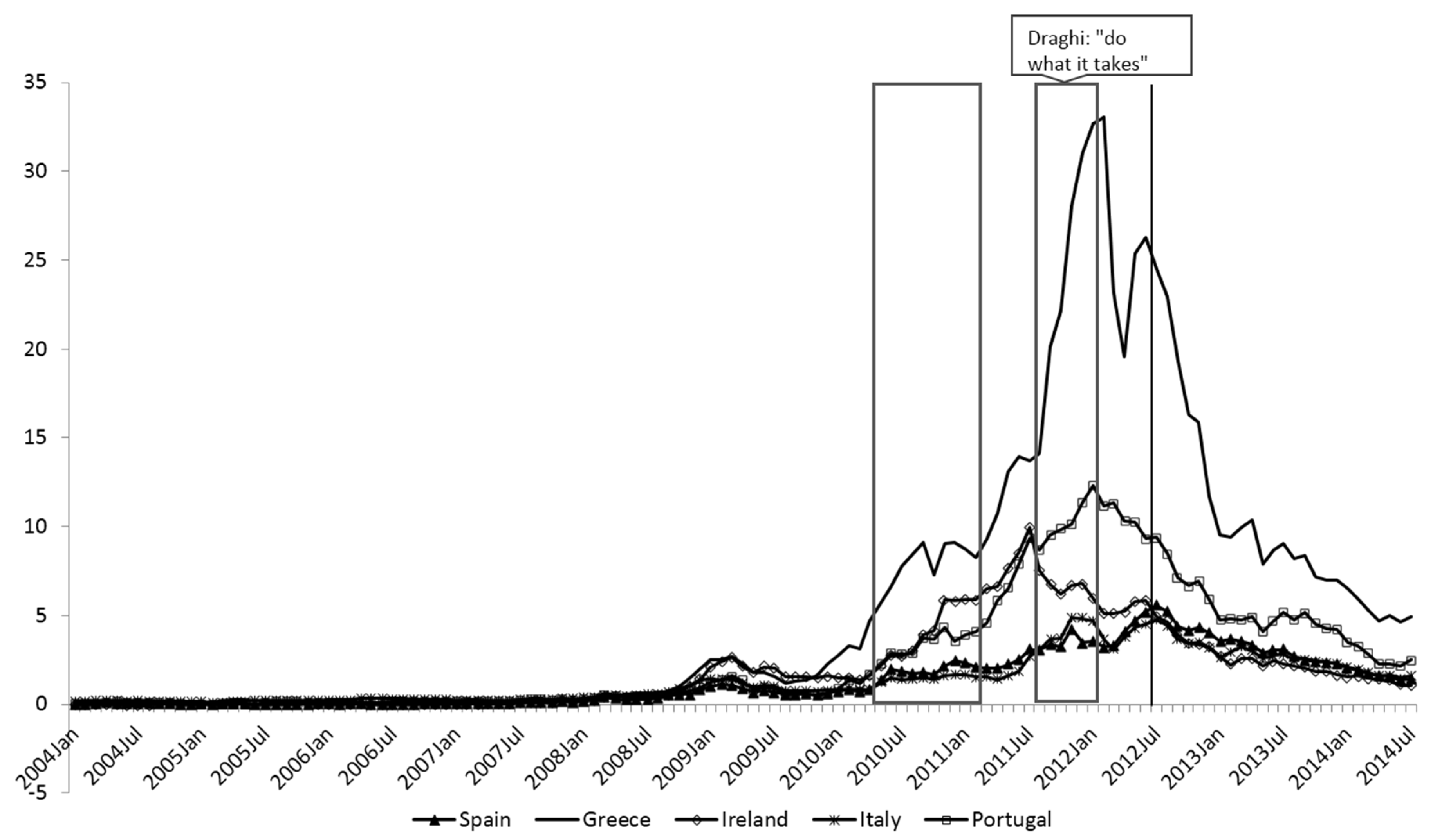
3. An Example Using the ECB’s Securities Market Program

In response to the global financial crisis, which erupted in 2007 with the collapse of the U.S. subprime market, and then intensified in September 2008 with the failure of Lehman Brothers, and the outbreak of the euro area’s sovereign debt crisis in late-2009 and early-2010, the ECB’s Governing Council adopted a number of non-standard measures to support financial conditions and credit flows to the euro area economy over and above what could be achieved through reductions in key interest rates. 33 Among those measures was the Securities Market Program (SMP). The SMP was launched in May 2010 as a response to the drying up of some secondary markets for government bonds. The aim of the program was to improve the functioning of the monetary policy transmission mechanism by providing depth and liquidity in segments of the sovereign bond market that had become dysfunctional. The program can, therefore, be thought of as a treatment for the malaise that was facing the financial system at the time.
In this section, we examine the effects of the SMP on spreads on Euro area sovereigns bonds for five Euro area stressed countries—Greece, Ireland, Italy, Portugal and Spain. There are thus five individuals, in the sense defined in our theoretical discussion above. Our data are monthly and cover the period from January 2004 through January 2013. 34 Previous studies have generally used dummy variables in an attempt to capture the effects of the program, with the exception of De Pooter, Martin and Pruitt [29], who approximate SMP purchases based on data available from Barclays as a counterparty to the ECB, and Eser and Schwaab [30] and Ghysels et al. [31] who use actual SMP purchases. We also use the actual amounts of sovereigns purchased under the program. These data are confidential, but were made available to us for use by the ECB. In contrast to most previous papers, we use monthly (rather than daily or intraday) data. There are two reasons why we use monthly data: (1) the confidential data on actual SMP purchases that were made available to us by the ECB are monthly; and (2) the use of monthly data allows us to control for the fundamental determinants of sovereign bond spreads.

Program Description

The SMP initially focused on the purchase of Greek, Irish and Portuguese government bonds; from August 2011, Spanish and Italian government bonds were also purchased. The impact of the program should thus have been felt most in sovereign debt markets in the stressed countries, causing the prices of sovereigns in these countries to rise and, thus, spreads (compared to the German bund) to fall. A total of 240 billion euros was spent during the course of the SMP transactions. Figure 1 shows the 10 year bond spreads for our five countries—Greece, Ireland, Italy, Portugal, and Spain. It also delineates two periods during which purchases were being made and the timing of the Draghi announcement (in July 2012) [32] that the ECB would do whatever was necessary to preserve the euro. As shown in the figure, the SMP took place at a time of rising spreads. Therefore, any simple correlation analysis would find that the effect of the SMP was to raise, rather than lower, spreads. Thus, finding the correct treatment effect is a matter of finding the unbiased coefficient in the presence of serious omitted variable and measurement errors. This is precisely what we claim our technique is able to do.
The basic relationship we are interested in evaluating (based on (12)) is
y i t = γ i t 0 + γ i t 1 x i t
where y i t is the spread on sovereign bonds in country i for period t and x i t is the SMP expenditure in country i in period t. This equation is our basic varying parameter Equation (12). As discussed earlier in this paper, each of the coefficients of (24) comprises a bias free component which we want to study. This component is corrupted by an effect for measurement error and omitted variable bias. We need to uncover the unbiased coefficient which will then be our estimate of y i t x i t , that is the partial derivative of spreads with respect to the amount of purchases under the SMP.
To estimate (24) we proceed as follows. Our data sample includes five countries: Greece, Ireland, Portugal, and Spain. Our monthly data cover the period from 2004M1 through 2014M7. We use the following equations for the coefficients—that is, these are the empirical counterpart to (13), the coefficient driver equations, where the coefficient drivers are chosen as a set of fundamental variables which are widely thought to determine the sovereign spreads
γ i t j = π j 0 + π j 1 R P i t + π j 2 G B i t + π j 3 P O L i t + π j 4 D G D P i t + π j 5 D E B T i t                        + π j 6 N E W S i t + ε i t
where RP is relative prices between the country in question and Germany, GB is the government fiscal balance relative to GDP for country i, POL is an indicator of political stability for country i, DGDP is the growth rate of GDP for country i, Debt is the stock of government debt relative to GDP for country i and NEWS is a measure of news effects with respect to the fiscal deficit of country i. 35 Detailed data definitions and sources are provided in Appendix.
Estimation of equation for γ 1 i 0 and γ 1 i 1 (i.e., the constant and the coefficient on SMP purchases in Equation (24)) yields the following results.
γ i t 0 = 1.96 + 97.5 R P i t 0.007 G B i t 0.09 P O L i t 55.4 D G D P i t + 0.03 D E B T i t ( 1.3 ) ( 13.6 ) ( 0.2 ) ( 0.6 ) ( 2.4 ) ( 3.0 ) 0.01 N E W S i t + ε i t ( 8.3 )
γ i t 1 = 0.0003 + 0.0009 P O L i t + 0.08 D G D P i t + 0.0000001 D E B T i t + 0.000001 N E W S i t + ε i t ( 0.2 ) ( 0.4 ) ( 0.7 ) ( 0 .006 ) ( 0.4 )
where the figures given in parentheses below each coefficient estimate are standard errors. Some variables had to be excluded from the second equation in order to estimate the above equations, because the SMP was only applied for a few months in each country resulting in an over-parameterization of the second equation. Since a number of these coefficients are insignificant, we successively restricted the driver equations based on the significance of variables following a general to specific methodology. The following model emerged.
γ i t 0 = 1.63 + 83.4 R P i t 0.14 P O L i t + 0.03 D E B T i t 0.01 N E W S i t + ε i t ( 1.4 ) ( 12.9 ) ( 1.1 ) ( 4.1 ) ( 8.4 )
γ i t 1 = 0.0002 + ε i t ( 0.23 )
As is evident, the effect of the SMP is constant and equal to −0.0002. Thus, our estimate of the unbiased (meaning, free of omitted-regressor and measurement-error biases) effect of the SMP on spreads is −0.0002 × SMP expenditure i t , as in (11). As there are no country specific variables in the second equation above, this implies that, in this case, the effect of the SMP programme is the same for each country. If there had been any variables remaining in the second equation, then our estimate of the bias free effect in each country would have been potentially different for each country.
To put the results into context, the largest amount spent on the program in any country in any single month was 47,590 million euros. Such a purchase would have lowered the spread by 9.5 percentage points (i.e., −0.0002 × 47,590) or 950 basis points. In other periods, where the purchases were less, the effect would have been correspondingly less. To put this into context, Eser and Schwaab [30] give a range of possible effects for an expenditure of 1 billion euros ranging from −1 basis point to −21 basis points. At the upper end, an expenditure of 47.5 billion euros would have reduced spreads by 997.5 basis points. 36 Ghysels et al. [31] report a long-run effect of the SMP within a range of 0.1 to 7 basis points for an expenditure of 100 million euros; thus, a purchase of 47,950 million would have led to a 3360 basis points fall in spreads, well above our findings that have been based on a varying-coefficient methodology and the actual purchases under the SMP.

4. Conclusions

The problem of estimating a general function with an unknown functional form can be solved without introducing a single specification error by changing this problem to one of estimating a corresponding relationship which is linear in variables but nonlinear in coefficients. Using this solution, we showed that the causal effects of a treatment on the treated individuals can be estimated. For this estimation, we use a real-world (i.e., misspecification-free) relationship between the treatment and its effect. The treatment’s effect depends on the definition of causality used. In our definition, causality is treated as a property of the real world. To measure the causal effect of a treatment on the treated individuals, we take the difference between the two real-world relationships, one for the effect of a treatment on a treated and another for the potential outcome of no treatment for the same individual. Obtaining pairs of treated and untreated individuals matched by similar propensity scores leads to specification errors.

Acknowledgments

We thank Fredj Jawadi and three referees for constructive comments.

Author Contributions

All authors contributed equally to the paper.

Conflicts of Interest

The authors declare no conflict of interest.

Appendix: Data Sources and Information

Spreads (in percentage points). 10-year benchmark on each country’s government 10-year bond yield minus the 10-year benchmark German government bond yield—ECB Statistical Data Warehouse—monthly average.
Covered-bond price indices. Euro area covered-bond price indices for bonds with any maturity and for those with greater than 10 years to maturity. Source: Thomson-Reuters DataStream.
Ratings. We take the ratings of each of the major credit rating agencies—Fitch, Moody’s, and Standard & Poor’s (S & Ps)—and construct a single series based on the agency that moved first. Ratings are mapped to a cardinal series running from 1 (AAA) to 22 (default).
Relative prices. Log difference of the monthly seasonally adjusted harmonized index of consumer prices (HICP) between each of the five countries and Germany—Thomson-Reuters DataStream.
Debt-to-GDP ratio. The ratio of the general government debt to GDP—quarterly data interpolated to monthly—Thomson-Reuters DataStream.
Political stability. We use the IFO World Economic Survey Index of Political Stability which takes values of between 0 and 10. A rise in the index implies greater stability.
Fiscal news. We construct real-time fiscal data, using the revisions to forecast general government budget balances published in the European Commission Spring and Autumn forecasts. Thus, for example, the revision to the Spring 2006 forecast is the forecast 2006 deficit/GDP ratio in the Spring compared to the forecast for 2006 made in the Autumn of 2005. This procedure allows us to generate a series of revisions (in percentage points), which, when cumulated over time, provides a real time cumulative fiscal news variable. We interpolate the series in such a way that news did not appear in the variable before it actually came out.
Economic activity. The rate of change of real GDP is interpolated to a monthly frequency—Thomson-Reuters DataStream.
SMP and CBPP. Data provided by the ECB.

References

  1. W.H. Greene. Econometric Analysis, 7th ed. Upper Saddle River, NJ, USA: Pearson/Prentice Hall, 2012. [Google Scholar]
  2. J.M. Wooldridge. Introductory Econometrics: A Modern Approach. Mason, OH, USA: Thomson South-Western, 2013, pp. 438–443. [Google Scholar]
  3. P.W. Holland. “Statistics and Causal Inference.” J. Am. Stat. Assoc. 81 (1986): 945–960. [Google Scholar] [CrossRef]
  4. P.A.V.B. Swamy, J.S. Mehta, G.S. Tavlas, and S.G. Hall. “Small Area Estimation with Correctly Specified Linking Models.” In Recent Advances in Estimating Nonlinear Models With Applications in Economics and Finance. Edited by J. Ma and M. Wohar. New York, NY, USA: Springer, 2014. [Google Scholar]
  5. P.A.V.B. Swamy, J.S. Mehta, G.S. Tavlas, and S.G. Hall. “Two Applications of the Random Coefficient Procedure: Correcting for misspecifications in a small-area level model and resolving Simpson’s Paradox.” Econ. Model. 45 (2015): 93–98. [Google Scholar] [CrossRef]
  6. P.A.V.B. Swamy, G.S. Tavlas, and S.G. Hall. “On the Interpretation of Instrumental Variables in the Presence of Specification Errors.” Econometrics 3 (2015): 55–64. [Google Scholar] [CrossRef]
  7. J.W. Pratt, and R. Schlaifer. “On the Interpretation and Observation of Laws.” J. Econom. Ann. 39 (1988): 23–52. [Google Scholar] [CrossRef]
  8. D. Rubin. “Estimating Causal Effects of Treatments in Randomized and Nonrandomized Studies.” J. Educ. Psychol. 55 (1974): 688–701. [Google Scholar] [CrossRef]
  9. D. Rubin. “Bayesian Inference for Causal Effects.” Ann. Stat. 6 (1978): 34–58. [Google Scholar] [CrossRef]
  10. J. Pearl. “An Introduction to Causal Inference.” Int. J. Biostat. 6 (2010): 1–59. [Google Scholar] [CrossRef] [PubMed]
  11. R.L. Basmann. “Causality Tests and Observationally Equivalent Representations of Econometric Models.” J. Econom. 39 (1988): 69–104. [Google Scholar] [CrossRef]
  12. B. Skyrms. “Probability and Causation.” J. Econom. Ann. 39 (1988): 53–68. [Google Scholar] [CrossRef]
  13. A. Zellner. “Causality and Econometrics.” In Three Aspects of Policy and Policymaking. Edited by K. Brunner and A.H. Meltzer. Amsterdam, The Netherlands: North-Holland Publishing Company, 1979, pp. 9–54. [Google Scholar]
  14. J. Pearl. Causality: Models, Reasoning, and Inference. New York, NY, USA: Cambridge University Press, 2000. [Google Scholar]
  15. A.S. Goldberger. Functional Form and Utility: A Review of Consumer Demand Theory. Boulder, CO, USA: Westview Press, 1987. [Google Scholar]
  16. J.J. Heckman, and D. Schmierer. “Tests of Hypotheses Arising in the Correlated Random Coefficient Model.” Econ. Model. 27 (2010): 1355–1367. [Google Scholar] [CrossRef] [PubMed]
  17. A. Yatchew, and Z. Griliches. “Specification Error in Probit Models.” Rev. Econ. Stat. 66 (1984): 134–139. [Google Scholar] [CrossRef]
  18. C.R. Rao. Linear Statistical Inference and Its Applications, 2nd ed. New York, NY, USA: John Wiley & Sons, 1973. [Google Scholar]
  19. I. Chang, C. Hallahan, and P.A.V.B. Swamy. “Efficient Computation of Stochastic Coefficients Models.” In Computational Economics and Econometrics. Boston, MA, USA: Kluwer Academic Publishers, 1992, pp. 43–53. [Google Scholar]
  20. I. Chang, P.A.V.B. Swamy, C. Hallahan, and G.S. Tavlas. “A Computational Approach to Finding Causal Economic Laws.” Comput. Econ. 16 (2000): 105–136. [Google Scholar] [CrossRef]
  21. P.A.V.B. Swamy, G.S. Tavlas, S.G.F. Hall, and G. Hondroyiannis. “Estimation of Parameters in the Presence of Model Misspecification and Measurement Error.” Stud. Nonlinear Dyn. Econom. 14 (2010): 1–33. [Google Scholar] [CrossRef]
  22. S.G. Hall, G.S. Tavlas, and P.A.V.B. Swamy. “Time Varying Coefficient Models; A Proposal for Selecting the Coefficient Driver Sets.” Macroecon. Dyn., 2016. forthcoming. [Google Scholar] [CrossRef]
  23. S.G. Hall, P.A.V.B. Swamy, G. Tavlas, (Bank of Greece), and M.G. Tsionas. “Performance of the time-varying parameters model.” Unpublished work. 2016. [Google Scholar]
  24. E. George, D. Sun, and S. Ni. “Bayesian stochastic search for VAR model restrictions.” J. Econom. 142 (2008): 553–580. [Google Scholar] [CrossRef]
  25. M. Jochmann, G. Koop, and R.W. Strachan. “Bayesian forecasting using stochastic search variable selection in a VAR subject to breaks.” Int. J. Forecast. 26 (2010): 326–347. [Google Scholar] [CrossRef]
  26. P.A.V.B. Swamy, and J.S. Mehta. “Bayesian and non-Bayesian Analysis of Switching Regressions and a Random Coefficient Regression Model.” J. Am. Stat. Assoc. 70 (1975): 593–602. [Google Scholar]
  27. C.W.J. Granger. “Non-linear Models: Where Do We Go Next—Time Varying Parameter Models.” Stud. Nonlinear Dyn. Econom. 12 (2008): 1–10. [Google Scholar] [CrossRef]
  28. P. Cour-Thimann, and B. Winkler. The ECB’s Non-Standard Monetary Policy Measures: The Role of Institutional Factors and Financial Structure. Working Paper Series 1528; Frankfurt am Main, Germany: European Central Bank, 2013. [Google Scholar]
  29. M. De Pooter, R.F. Martin, and S. Pruitt. The Liquidity Effects of Official Bond Market Intervention. International Finance Discussion Papers; Washington, DC, USA: Board of Governors of the Federal Reserve System, 2015. [Google Scholar]
  30. F. Eser, and B. Schwaab. Assessing Asset Purchases within the ECB’s Securities Markets Programme. ECB Working Paper No. 1587; Frankfurt, Germany: European Central Bank, 2013. [Google Scholar]
  31. E. Ghysels, J. Idier, S. Manganelli, and O. Vergote. A High Frequency Assessment of the ECB Securities Markets Programme. ECB Working Paper, No. 1642; Frankfurt, Germany: European Central Bank, 2014. [Google Scholar]
  32. M. Draghi. “Speech by the President of the European Central Bank at the Global Investment Conference in London.” 26 July 2012. Available online: https://www.ecb.europa.eu/press/key/date/2012/html/sp120726.en.html (accessed on 22 January 2016).
  • 1For textbook expositions, see Greene [1] (pp. 888–896) and Wooldridge [2] (pp. 438–443).
  • 2See Holland [3].
  • 3For a short discussion on these issues, see Greene [1] (pp. 893–895).
  • 4As we explain below, the coefficients and error term of a linear-in-variables and nonlinear-in-coefficients model are unique in the sense that they are invariant under the addition and subtraction of the coefficient of an omitted regressor times any included regressor on its right-hand side. Swamy, Mehta, Tavlas and Hall [4,5] showed that models with nonunique coefficients and error terms are misspecified.
  • 5This is what Greene [1] (pp. 888–889) calls “the treatment effect in a pure sense.”
  • 6See, for example, Swamy, Tavlas and Hall [6].
  • 7Most empirical studies use a treatment dummy to derive the impact of the treatment; the dummy variable takes the value 1 for the treated individuals and 0 for the untreated individuals.
  • 8In doing so, Pratt and Schlaifer [7] followed Rubin [8,9].
  • 9Greene [1] (p. 888) pointed out that “The natural, ultimate objective of an analysis of a “treatment” or intervention would be the effect of treatment on the treated.”
  • 10Greene [1] (p. 894) pointed out that the desired quantity is not necessarily the ATE, but ATET.
  • 11Skyrms distinguished among different types of causation such as deterministic, probabilistic, and statistical. He argued that the answers to questions of probabilistic causation given by different statisticians depended on their conceptions of probability. Three major concepts of probability are: rational degree of belief, limiting relative frequency, and propensity or chance. Skyrms [12] (p. 59) recognized that not all would agree with the subjectivistic gloss he put on the causal approaches of Reichenbach, Granger, Suppes, Salman, Cartwright and others. As Skyrms pointed out, “statistical causation is positive statistical relevance which does not disappear when we control for all relevant pre-existing conditions.” We consider this definition of statistical causation here. Skyrms further clarified that “Within the Bayesian framework … “controlling for all relevant pre-existing conditions” comes to much the same as identifying the appropriate partition … which together with the presence or absence of the putative cause (or value of the causal variable) determines the chance of the effect.”
  • 12The list of these misspecifications is given in Section 2.2.6 below.
  • 13In his causal analyses, Pearl [14] used the Bayesian interpretation of probability in terms of degrees of belief about events, recursive models, and in many cases finitely additive probability functions. Pearl’s [14] (p. 176) Bayesian view of causality is that “[i]f something is real, then it cannot be causal because causality is a mental construct that is not well defined.” This view is not consistent with Basmann’s [11] view, which is also the view that we adopt in this paper.
  • 14The principle of causal invariance (Basmann [11] (p. 73)): Causal relations and orderings are unique in the real world and they remain invariant with mere changes in the language we use to describe them. Examples of models that do not satisfy this principle are those that are built using stationarity producing transformations of observable variables (see Basmann [11] (p. 98)). A related principle is that causes must precede their effects in time. Pratt and Schlaifer [7] (pp. 24–25) pointed out an interesting exception to this principle which is: “Whether or not a cause must precede its effect, engineers who design machines that really work in the real world will continue to base their designs on a law which asserts that acceleration at time t is proportional to force at that same time t.” The reason why we consider real-world (misspecification-free) relationships is that they satisfy the principle of causal invariance. They do not disappear when we control for all relevant pre-existing conditions, see Skyrms [12] (p. 59). We build misspecification-free models with these properties. If we do not estimate y 1 i * y 0 i * from the misspecification-free relations of y 1 i * and y 0 i * , then according to Basmann [11], our estimate of the treatment effect y 1 i * y 0 i * will not be an estimate of the causal effect of a treatment on the treated ith individual.
  • 15We do not treat measurement errors as random variables until we make some stochastic assumptions about them.
  • 16The reason for assigning this label to them is that they are included as regressors in our regressions below.
  • 17Data on x 1 i , K + 1 * are not available in some experiments like medical experiments. In these cases, what all we know is whether an individual is treated or not (see Greene [1] (pp. 893–894)). In these cases it is possible to obtain analytical expressions but not numerical measures for the treatment effects.
  • 18The reason why we attach this label to them is that they are actually omitted from our regressions below.
  • 19Unobserved treatment variable: In the absence of data on x 1 i , K + 1 , the coefficient of a dummy variable is used to measure treatment effects, as in the Heckman and Schmierer’s (HS) [16] model. Greene [1] (pp. 251–254, 893) elaborated on this practice by commenting that though a treatment can be represented by a dummy variable, measurement of its effect cannot be done with multiple linear regression
  • 20One result that can be derived from (6)–(9) is the following: Consider two competing models of the same dependent variable with unique coefficients and error terms. Let each of these models be written in the form of (6) and let some continuous regressors be common to these two models. Of the pair of coefficients on a common regressor in the two models, the one with smaller magnitudes of omitted-regressor and measurement-error biases will be closer to the common true partial derivative component of the pair. This correct conclusion could not be drawn from the J test of two separate families of hypotheses on a misspecified model (see Greene [1] (p. 136)).
  • 21A proof of this statement follows from Pratt and Schlaifer’s [7] (p. 34) statement that “… some econometricians require that … (the included regressors) be independent of ‘the’ excluded variables themselves. We shall show … that this condition is meaningless unless the definite article is deleted and can then be satisfied only for certain “sufficient sets” of excluded variables …”
  • 22A proof of this statement is given in Swamy et al. [4] (pp. 217–219).
  • 23We call the coefficients of (12) “the random coefficients” but not “random parameters.” The reason is that there are only coefficients and no parameters in (12). We call the coefficients of (13) “the fixed parameters” to distinguish them from those of the fixed-coefficient versions of (12). We do not use the word “random parameters,” since it creates confusion between (12) and its fixed coefficient versions.
  • 24The definition of coefficient drivers differs from the definition of instrumental variables. The latter variables do not explain variations in the coefficients of (12) as do coefficient drivers. The coefficient for any regressor in (12) is partly dependent on the coefficient drivers in (13). In instrumental variable estimation, first, the instrumental variables are used to transform both the dependent variable and the explanatory variables and then the transformed variables are used to estimate the coefficients to the regressors.
  • 25The functional form of (13) is different from that of (8) or of (7) and (9). We will correct this mistake in Equation (21) below.
  • 26A similar admissibility condition for covariates is given in Pearl [14] (p. 79). Pearl [14] (p. 99) also gives an equation that forms a connection between the opaque English phrase “the value that the coefficient vector of (12) would take in unit i, had X 1 i = ( X 1 i 1 , ... , X 1 i , K + 1 ) been x 1 i = ( x 1 i 1 , ... , x 1 i K + 1 ) ” and the physical processes that transfer changes in X 1 i into changes in y 1 i .
  • 27A clarification is called for here. In (12), the number of the vectors of K + 2 coefficients increases with the number of individuals in the cross-sectional sample. So many coefficients are clearly not consistently estimable. However, in (14) below, the number of unknown coefficients ( Π 1 ) is only (K + 2) × ( p + 1). This number does not increase with n 1 . So, the trick that makes our estimation procedure yield a consistent estimator of Π 1 is to include the same set of coefficient drivers across all the coefficient equations in (13) and impose appropriate zero restrictions on the elements of Π 1 if different sets of coefficient drivers are needed to estimate different components of the coefficients of (12).
  • 28Any variables that are highly correlated with x 1 i will also be correlated with both the regression part, x 1 i Π 1 z 1 i , and the random part, x 1 i ε 1 i , of the dependent variable, y 1 i , of Equation (14). Furthermore, this equation is the end result of the sequence of Equations (1)–(6), and (13) that is used to avoid specification errors (i)–(iv) of Section 2.2.6. These two sentences together prove that the avoidance of specification errors (i)–(iv) leads to the nonexistence of instrumental variables. There is no contradiction between this result and Heckman and Schmierer’s [16] (p. 1356) instrumental variables approach because in this paper, no use is made of their threshold crossing model which assumes separability between observables Z that affect choice and an unobservable V. Their instrumental variable is a function of Z.
  • 29The formulas for these estimators and predictors are given in Chang, Hallahan, and Swamy [19] and Chang, Swamy, Hallahan and Tavlas [20]. The sampling properties of ( Π ^ 1 , σ ^ 1 ε 2 Δ ^ 1 ε ) are studied in Swamy, Tavlas, Hall and Hondroyiannis [21].
  • 30We consider below the cases where these quantities are unknown.
  • 31Swamy and Mehta [26] originated the theorem stating that any nonlinear functional form can be exactly represented by a model that is linear in variables, but that has varying coefficients. The implication of this result is that, even if we do not know the correct functional form of a relationship, we can always represent this relationship as a varying-coefficient relationship and thus estimate it. Granger [27] subsequently confirmed this theorem.
  • 32This bias depends on a linear specification. It also depends on a non-zero correlation between the omitted regressor and the included regressors.
  • 33Asset purchase programs were a part of the ECB’s overall response to the two crises. For detailed review of the ECB’s responses, see Cour-Thimann and Winkler [28].
  • 34We start our estimation well before the beginning of the SMP program as we believe the longer sample period is helpful in determining the other parameters of the model and hence gives us a more accurate set of parameters to remove the omitted variable bias. We choose to use monthly data as most of the fundamental driver variables are only available at a monthly frequency.
  • 35NEWS is calculated from updates to forecasts of the general government balance found in the EC’s spring and autumn forecasts.
  • 36It is difficult to make a comparison with the results of De Pooter, Martin and Pruitt [29] because they define their SMP variable as a percentage of outstanding debt rather than the absolute value of purchases. As far as we can discern, their result seems to yield a similar order of magnitude to our measure.
Figure 1. Spreads on 10-year government bonds over 10-year bonds (in percentage points).
Econometrics 04 00019 g001

