1. Introduction
Most empirical studies analyze the effects of income distribution determinants through decomposition methodologies based on Oaxaca-Blinder (1973) [
2,
3]. Those methodologies usually focus on the wage distribution of a single individual assuming that all employment decisions are made in an isolated or independent way with respect to other household members. Notwithstanding, the literature on intra-household labor supply shows several models of the interdependence in the employment decisions within the household. Assortative mating literature provides vast evidence of interrelations of individual variables among members, such as their education levels, labor income, the choice of hours of work,
etc. Ignoring this feature when estimating household labor earnings on decomposition exercises provides a scenario that may be biased or unrealistic.
The main component of personal earnings is labor income. Therefore, it is important to know its intra-household determinants to understand the behavior of the household incomes and their consequences on inequality. In the most traditional model, there is a sole individual responsible for making labor decisions independently of other household members. However, in the case of complete households (with head and spouse) it is usual that this decision is made by the couple. There are several models in the literature where a couple faces the problem of deciding together their labor supply according to their interests within the home (e.g., Chiappori and Pierre-Andre, 1992 [
4]; Blundell
et al., 2005 [
5]; van Klaveren
et al., 2008 [
6], among others). The main mechanisms behind this decision are the reservation wages of each member and the bargaining power that determines the share rule of the household income.
Given the complexity involved in analyzing the joint employment decisions of all household members, the usual alternative is to focus only on the decisions made by the household head and spouse. The implicit assumption is that the rest of the household members will not change their behavior, or at least their impact on family income is small. This assumption may be too simple, but it is a starting point used in the literature to understand the complex mechanisms interacting in the labor decisions made within the household. In particular, both the reservation wages and bargaining power depend on observable and unobservable characteristics of household members such as age, education status, persuasion, etc. Modeling both earnings equations to analyze household income distribution while taking into account their interactions requires a methodology that generates counterfactual distributions of hypothetical changes on their determinants.
Some examples of models including employment decisions within the household are Browning
et al. (1994) [
7], Gasparini and Marchionni (2007) [
8], Galiani and Weischenbaum (2012) [
9], among others. Usually these studies make several parametric and/or distributional assumptions, such as normality in the unobservable income determinants. This approach could be too strict or it may not be quite representative of the actual income distribution. Another usual methodological aspect is that those papers use models focused on conditional means, relying on parametric assumptions other aspects of the distribution. Despite the progress of quantile regression literature allows exploring issues beyond the average effects, the bulk of the decompositions literature is based on counterfactual distributions of earnings equations for a single individual (
i.e., Machado and Mata (2005) [
10], Melly (2005) [
11] and Firpo
et al. (2009) [
12]). This paper attempts to expand this literature by proposing a methodology to generate counterfactual scenarios on bivariate distributions using conditional quantiles.
The main contribution of this paper is to show that the problem of generating counterfactual income distributions for both household members is just an exercise of numerical integration involving a joint mechanism to generate a pair of random variables through their marginal distributions. Once this mechanism is established, it is possible to use the ranking association of both household members in order to get a set of replicates or realizations of the joint distribution. Nevertheless, the fact that incomes are related with observable characteristics makes necessary to introduce some structure to the conditional income distribution. Conditional quantiles are useful to model this matter for two reasons: first, they are the counterpart of the cumulative conditional distribution, and second they are easily estimable by standard methods. Quantile regressions allows an indirect way to capture the unobservable heterogeneous effects on each marginal distribution. Finally, the last step of the proposed method is to incorporate the relationship between the conditional incomes of both household members using a probabilistic association of conditional rankings.
The paper is organized as follows. In
Section 2, a methodology to simulate bivariate random variable realizations based on marginal distributions is presented.
Section 3 extends this idea to conditional joint distributions and its applications to counterfactual distributions.
Section 4 shows an empirical application with household survey data for different countries in the Southern Cone of Latin America. Finally,
Section 5 discusses the results and scope of the methodology.
2. Generating Random Variables
Generating random variables in the univariate case is relatively simple, and there are several methods available. The most widely used is the inverse cumulative function method: let
U be a random variable with a uniform distribution
, then the transformation
generates a random variable with distribution
. Thus, this procedure simply consists on taking a realization of a uniform random variable
u and then computing the
u quantile
. In the case of integer variables, the logic is quite similar to the continuous case (Devroye, 1986) [
13].
The bivariate setup is more complex because the statistical relationship between two variables must be considered. A closely related problem can be found in the study of copula functions. A copula is a function that links the joint distribution to the one-dimensional marginal distributions (Nelsen, 1999) [
14]. As in the univariate case, there are several methods to create a bivariate random draw. For example, the conditional distribution method allows to generate a random vector
using a vector
of independent uniform random variables. Specifically, the method of the conditional distribution requires the following two steps: (1) compute
, where
is the marginal cumulative distribution of
; and (2) compute
, that is, using the inverse of the cumulative distribution of
conditional on
. The key to this process is to know the exact functional form of the conditional distribution, which can be too strict in practice.
Another strategy that allows us to adapt the univariate methods (such as the inverse cumulative function) to the bivariate problem is the grid method. Before explaining this procedure, it is appropriate to give some definitions.
Definition 1. (encoder function). Let and be two integer variables in the domain and , respectively. We define the encoder function as .
The image of this function is
. The most interesting property of the encoder function is that it has a single value
m for each ordered pair
. Therefore, each coordinate is identified by the following decoding function:
Property 1. (decoding functions). Let be a encoder function. Then, the coordinates and can be obtained from the decoding functions: and .
The last element that is needed is to define the set of grids of an enclosure
Definition 2. (grid ). Let be an enclousure, a grid is defined as with , , where and are values such that they satisfy ; and .
Finally, consider two random variables
with a joint density function
. To generate a realization of a vector
from the population distribution
we can use the grid method by following the next steps:
Subdivide the enclosure A in grids , where .
Calculate the probability mass of each grid for every m.
Generate a realization of an integer univariate random variable with probability distribution , calculated in the previous step.
Decode to obtain the vector .
Compute the realization of assigning values within the grid .
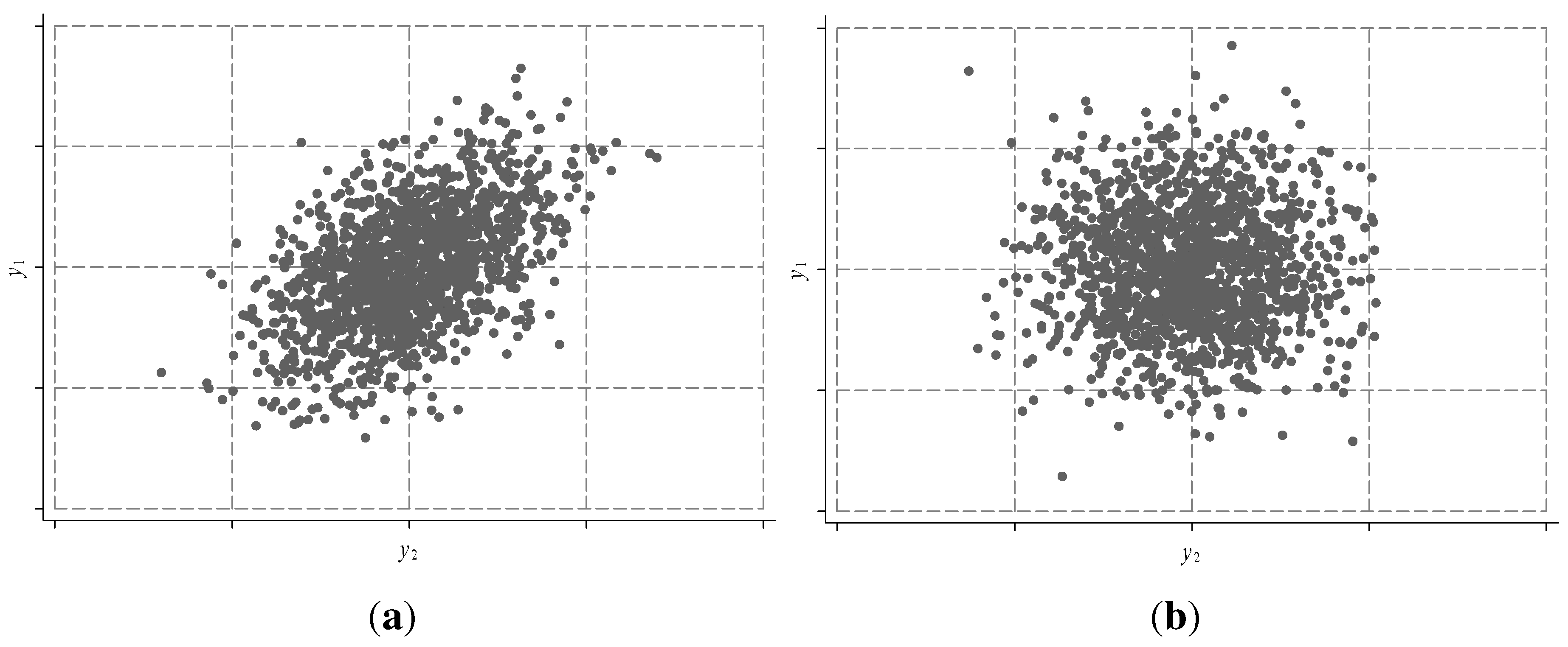
Figure 1 presents two examples to illustrate how the method works: graph
(a) shows the situation of two random variables with a positive relationship while
(b) represent the independent relationship case.
Figure 1.
Random variables and correlation.
Figure 1.
Random variables and correlation.
The dotted lines delimit the grids subdividing the enclosure (
i.e., the support of both random variables). Clearly, in the first case the probability mass (measured by the proportion of points falling into each grid) is concentrated in the diagonal given by the bisectrix, while in the second case there is no clear pattern for the joint probability. Logically, the greater the number of grids, the better the approach of the method (Hörmann
et al., 2004 [
15]). Therefore, the method incorporates the statistical relationship between
and
through the probability of each grid.
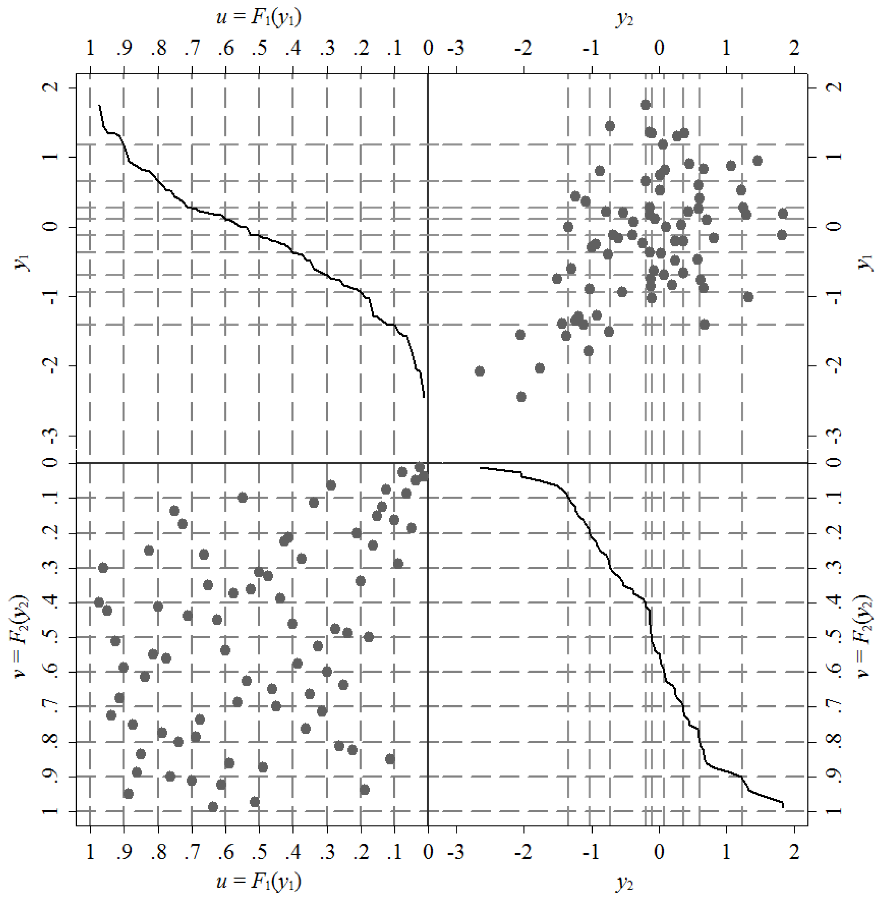
Lastly, note that the grids can be determined by their marginal quantile by defining the values
and
. The validity of this equivalence is that the cumulative distribution is an increasing monotonic transformation of the random variable support. In other words, the
value represents the ranking position resulting from sorting the
s increasingly. This establishes a one to one relationship between any value of
and its ranking. Then, the grid
can be written as:
Figure 2 shows this equivalence in the definition of grids. The top graph on the right shows the point cloud in the plane
, while the lower graph on the left shows its counterpart in the plane
. The figures in the other two quadrants show the cumulative probability of each variable viewed solely as a univariate distribution (marginal distribution). Note that although the scales of the enclosures are different, each point belonging to a grid in the upper right quadrant has a corresponding grid on the lower left quadrant.
Figure 2.
Equivalence of grids.
Figure 2.
Equivalence of grids.
The grid definition on the marginal probability plane is equivalent to define the grid in terms of the levels of both variables. Then, looking at the grid plane makes it possible to adapt this method to the context of conditional quantiles. This is a key idea because it is precisely the estimation target of the quantile regression technique. Briefly, building the link between the probability grids and the conditional quantiles allows us to associate the marginal rankings with the univariate method of random sampling for the purpose of generating counterfactual distributions. Furthermore, this strategy requires less information than the method of the conditional distribution given that it only requires to know the probability of each grid rather than an entire functional form for the distribution of conditional on .
4. Empirical Illustration
In this section we use real data as an application of the proposed methodology to generate counterfactual distributions of per capita household income. The model is defined by Equations (1) and (2) where
and
represent the labor earnings (in logs) of the household head and spouse, respectively. The vectors
and
are observed characteristics (age, education, gender, number of children) while
and
are terms representing the unobserved determinants of earnings. We focus our analysis on five countries in Latin America, particularly those belonging to the Southern Cone: Argentina, Brazil, Chile, Paraguay and Uruguay. The data come from household surveys collected by the statistical institutes of each country.
3We use three alternative methods to estimate the earning models. The first method is to use a seemingly unrelated regression model (SUR), in which the parameters in Equations (1) and (2) are estimated by OLS but allowing correlation between the error terms in both equations. The second case is the estimation of a quantile regression model (IQR), in which the assumption is that the error terms are independent. Finally, the outcomes from these methods are compared with those obtained by applying the methodology of estimating through quantile regressions but relating the model equations using the grids method (DQR).
The first exercise is to analyze the performance of the proposed methodology (DQR) relative to the other two strategies (SUR and IDR). We use an
ad-hoc rule to choose the number of quantiles on each earning equation. This rule ensures that the number of observations on each grid will be around 40 in the case in which both equations are independent.
4 The reason behind choosing this rule is to try to get reliable estimates of each grid without losing the asymptotic properties.
Using these three methods, the model’s coefficients are estimated in order to generate the joint distribution of labor earnings of the heads and spouses in a particular year. These earnings are used to build a new household per capita income and compute the Gini coefficient.
Table 1 shows the results. The first panel of the table shows the Gini coefficient observed in each country, followed by the Gini coefficient of the simulated income from each method. The standard errors of each coefficient are computed using 50 simulation replicates. Errors in the SUR model are generated 50 times from a bivariate normal distribution using all the estimated parameters. For the IQR, uniform random variables are generated independently, so that there is no conditional ranking association. Finally, under the DQR simulation, the values of the labor earnings of the head and spouse are obtained from the estimated probabilities in the grid method, namely considering the relationship between the two equations. The second panel in the table presents the mean square error (MSE) of each estimate with respect to the empirical distribution:
Table 1.
Performance.
| | Argentina | Brazil | Chile | Paraguay | Uruguay |
|---|
| Gini | | | | | |
| Observed | 48.78 | 56.33 | 54.65 | 52.96 | 46.81 |
| OLS | 49.12 | 54.61 | 52.54 | 53.19 | 46.22 |
| | (0.03) | (0.01) | (0.02) | (0.05) | (0.02) |
| IQR | 48.25 | 55.88 | 54.22 | 52.02 | 46.30 |
| | (0.01) | (0.00) | (0.02) | (0.02) | (0.01) |
| DQR | 48.34 | 56.05 | 54.38 | 52.32 | 46.44 |
| | (0.01) | (0.00) | (0.02) | (0.01) | (0.01) |
| ECM | | | | | |
| OLS | 0.16 | 2.96 | 4.46 | 0.18 | 0.38 |
| IQR | 0.28 | 0.20 | 0.20 | 0.90 | 0.26 |
| DQR | 0.20 | 0.08 | 0.09 | 0.43 | 0.14 |
| Obs. | 16571 | 78188 | 45915 | 3337 | 10907 |
The SUR method has the lowest MSE for Argentina and Paraguay, followed closely by the DQR method. Therefore, in these two cases, using the conditional mean with an assumption of normality in errors fits relatively well to the real data. In the cases of Brazil, Chile and Uruguay the method that achieves the lowest MSE is the DQR, followed by the IQR method. As discussed above, these results suggest that the DQR method requires a certain amount of observations to achieve relatively good performance. However, in the case of Uruguay, which has a smaller sample than Argentina, DQR method has the lowest MSE. Then, this methodology may also depend on how well the model fits to the empirical distribution. However, large sample sizes should improve the approximation of the DQR method.
The next step in this section is to perform the micro-decomposition discussed in
Section 3.3 in order to compare the results obtained with the three methods. As an illustration, we estimate the parameters effect in the equations of labor earnings.
Table 2 shows the results of this exercise: the row Δ Obs contains the observed variation in the Gini coefficient for the entire period. The first panel in the table shows the parameters effect in the earning equation of the head, the second presents the effect corresponding to the spouse equation, and the third panel shows the decomposition of the parameters effect in both equations.
The greatest variation in the Gini coefficient corresponds to Argentina, with a fall of almost 8 points, followed by Uruguay with about 7 points. Brazil and Chile also show a reduction in inequality in terms of the Gini coefficient with values slightly higher than 4 points, while in the case of Paraguay an increase of around a point is observed. The estimation results are interpreted as follows: the value −1.0 of the parameters effect in the equation of the spouse in Argentina under the SUR model indicates that if all that would have changed between 2004 and 2012 were the parameters governing the equation of the spouse of the household, the Gini coeficient would had been reduced by a point.
Table 2.
Parameters Effects
Table 2.
Parameters Effects
| | Argentina | Brazil | Chile | Paraguay | Uruguay |
|---|
| | 2004–2012 | 2004–2012 | 2003–2011 | 2007–2011 | 2004–2012 |
|---|
| Δ Obs | −7.8 | −4.1 | −4.4 | 1.0 | −6.8 |
| Head | | | | | |
| OLS | −1.0 | −1.2 | 1.9 | 0.0 | −1.0 |
| | (0.01) *** | (0.00) *** | (0.01) *** | (0.01) *** | (0.01) *** |
| IQR | −0.7 | −0.7 | −1.1 | −0.5 | −1.3 |
| | (0.01) *** | (0.00) *** | (0.01) *** | (0.02) *** | (0.01) *** |
| DQR | −0.6 | −0.6 | −1.1 | −0.8 | −1.4 |
| | (0.01) *** | (0.00) *** | (0.01) *** | (0.02) *** | (0.01) *** |
| Spouse | | | | | |
| OLS | −1.2 | −0.7 | 1.0 | 0.3 | −0.6 |
| | (0.01) *** | (0.00) *** | (0.01) *** | (0.01) *** | (0.01) *** |
| IQR | −0.3 | −0.1 | 0.4 | −0.1 | 0.2 |
| | (0.00) *** | (0.00) *** | (0.01) *** | (0.02) *** | (0.00) *** |
| DQR | −0.4 | −0.1 | 0.3 | −0.3 | 0.2 |
| | (0.00) *** | (0.00) *** | (0.00) *** | (0.02) *** | (0.00) *** |
| Both | | | | | |
| OLS | −2.3 | −1.7 | 2.9 | 0.3 | −1.6 |
| | (0.01) *** | (0.01) *** | (0.01) *** | (0.01) *** | (0.01) *** |
| IQR | −1.1 | −0.4 | −0.7 | −0.5 | −1.0 |
| | (0.01) *** | (0.00) *** | (0.01) *** | (0.02) *** | (0.01) *** |
| DQR | −1.1 | −0.3 | −0.8 | −0.9 | −1.1 |
| | (0.01) *** | (0.00) *** | (0.01) *** | (0.03) *** | (0.01) *** |
The greatest discrepancies among methodologies belong to the SUR method, while the IQR and DQR do not differ significantly from each other. The differences between the DQR and IQR are between 0 and 0.1 points (in absolute value) in the countries where the DQR achieves the lowest MSE. This result suggests a significant difference in terms of effects (between 0% and 30% in some cases). However, the economic significance of these differences is small (one tenth point of the Gini). The case of Paraguay shows a potential weakness in the DQR method when there are too few observations available. Since DQR has the lowest MSE in this country, the differences with the other methods suggest that with small samples the DQR method could present a potential bias in the estimated effects.
5. Conclusions
This paper proposes a method to incorporate the intra-household relationship between the labor incomes of the head and the spouse in decomposition studies. The paper closely follows the articles of Machado and Mata (2005) [
10] and Melly (2005) [
11]. We try to extend these papers by incorporating the correlation of intra-household income modeled by a simultaneous equation system. The key idea in our proposal is to associate conditional quantiles by adapting an standard method for generating random variables: the grid method.
The complexity associated with the joint employment decisions in a household leads us to focus our analysis on the behavior of the head and spouse, independently of the decisions of the rest of the family members. Furthermore, our model only analyzes the determination of labor earnings, assuming all other sources of income remain unchanged. Incorporating these other sources is an exercise that does not allow certain generalizations because non-labor income depends mainly on the social policies applied in each country (Badaracco, 2014 [
19]).
An empirical application performing a simple decomposition exercise was implemented by using data from household surveys for the Southern Cone countries in Latin America. The counterfactual scenarios considered consisted on a change in the parameters in the labor earnings equations in two different moments in time. The results show that, in general, incorporating the interaction of household incomes substantially improves the goodness of fit to the empirical income distribution. Also, using quantile regression can dramatically change the results of the simulation exercise. However, although the introduction of correlation in incomes yields different results, the economic significance seems to be minor. The comparative exercise among different surveys shows that the performance of the method clearly depends on the sample size by limiting the number of grids. Moreover, given the sample size, the goodness of fit of the semiparametric method seems to be another key point.
The paper omits some important issues related to the estimation of earnings equations such as sample selection and endogeneity of covariates (e.g., education). The main reason for doing this is that our target is to propose a methodology for the generation of counterfactual distributions, showing their application using standard regression methods developed in the literature. Solving all these problems requires the use of more specific methodologies that are still under development such as those in Buchinsky (2001) [
21] and Chernozhukov and Hansen (2006) [
22]. Exploring the performance of the proposed method under these estimation techniques is postponed for future research.


