1. Introduction
There are different interpretations of the extremal index (θ) in the literature on extreme value theory for weakly dependent processes. This concept, originated in papers by Loynes [
1] and O’Brien [
2] and developed in detail by Leadbetter [
3], reflects the effect of clustering of extreme observations on the limiting distribution of the maximum. Thus, the first author showed that
with
,
,
a normalizing sequence and
F the unconditional distribution function of a sequence of weakly dependent random variables
; see also [
4,
5]. In a similar spirit, [
6] showed that the presence of clustering affected the limiting distribution of block maxima,
i.e.,
with
,
determining a partition of the sample of length
n, such that
and
.
Alternatively, Leadbetter [
3] showed that for stationary sequences exhibiting short range dependence, the inverse of the extremal index is the limiting mean number of exceedances of
in an interval of length
. This result mathematically reads as follows
with
the indicator function. By stationarity, this property is satisfied for any block of
consecutive elements defined in the sequence.
Inference about the extremal index parameter has also been extensively studied. The most popular estimators are the logs method, obtained from operating with the asymptotic results of the distribution of the maximum, the runs method derived from operating with (2) and the blocks method obtained from (3). For a careful review of these and other related estimators proposed in the literature, see [
5,
7,
8]. Alternative estimation techniques recently developed are [
9,
10,
11,
12]. Finally, for a review of the underlying probability theory, the interested reader can consult [
13] or, more recently, [
14].
Our first aim in this paper is to build on the results of Leadbetter given in (3) about cluster size and to introduce an alternative characterization of θ as a limiting probability characterized by two Poisson processes. This characterization allows an intuitive and simple estimation procedure. Instead of focusing on the cluster size of extremes in a sequence, our characterizing condition of θ focuses on an extra level
satisfying the following property
We will see that this condition implies that the ratio of exceedances of
and
by the sequence of block maxima converges asymptotically to θ.
This characterization of the extremal index as a limiting probability naturally yields a family of estimators that is consistent and converges, after proper standardization, to a normal distribution. This result is new in the extreme value theory literature. In fact, most estimators of θ proposed in the literature are inconsistent as the sample size increases. This is due to the Poisson property inherited from the choice of extreme levels for defining the extremal index estimator. A few exceptions are the estimators of θ proposed in [
9,
15] and, more recently, [
14]. The first author solves this problem by using lower levels that allow one to benefit from increasing sample sizes and also by introducing a standardizing sequence that corrects for increasing cluster sizes. In [
15], using this sequence, a variant of the blocks method is proposed that is asymptotically normal. In a similar context, Novak and Weissman [
9] also prove the consistency and asymptotic normality of the blocks and runs methods. Robert [
14] introduces estimators of the limiting cluster size probabilities, which are constructed through a recursive algorithm. This author derives estimators of the extremal index and studies their asymptotic and finite-sample properties. Other recent articles generalizing the extreme value theory to models with serial dependence are, for example, [
16,
17,
18].
In this paper the characterization of θ and the subsequent estimator determined by two levels makes statistical inference about the θ parameter possible in a simpler manner. Interestingly, the estimation procedure is straightforward and not very sensitive to the practical choice of the block length and threshold
for fixed sample sizes. Similar strategies are pursued in [
9,
15] and, more recently, [
14]. We also show in an extensive simulation study that the nominal coverage of our estimator obtained from the asymptotic normal distribution is very good for small sample sizes. Finally, our estimator fares very well in a comparison of finite samples among the logs, blocks and runs methods for a wide class of time series exhibiting clustering of extremes and widely discussed in the literature.
The paper is structured as follows.
Section 2 discusses the new characterization of the extremal index.
Section 3 introduces the family of estimators of θ and its asymptotic properties. In
Section 4, we illustrate these asymptotic results with a simulation experiment for time series exhibiting clustering of extreme values. In
Section 5, our alternative estimation method is applied to test for the presence of clustering of extremes in monthly macroeconomic time series of unemployment growth and inflation rates in the United States.
Section 6 concludes.
2. Characterization of the Extremal Index
It is well known for sequences of independent and identically distributed (i.i.d.) random variables following an unknown distribution
F that, under some regularity conditions, the asymptotic distribution of the sample maximum is non-degenerate. In particular, for some suitable constants
,
, we have that
where
G is the relevant limiting distribution function that must be one of the following types (see [
19]),
- Type I: (Gumbel)
.
- Type II: (Fréchet)
- Type III: (Weibull)
Taking logs in both terms of (5) and denoting
, we observe that
with
a positive real function defined by the exponent of any of the three extreme value distributions introduced above.
For large
n and
sufficiently high, Equation (6) is sufficient to define a family of random variables
indexed by
x that converges in distribution to a family of Poisson random variables with mean
; see [
20,
21]. For the sake of simplicity in the exposition, we will assume hereafter
x fixed and will use
to denote the threshold sequence
. Similarly,
denotes the corresponding random variable.
These important and well-known results of extreme value theory (
evt ) can be extended to study the maximum of a wide class of dependent processes. We concentrate here on stationary sequences where the extent of long-range dependence is restricted by a distributional mixing condition
introduced in [
3]. This mixing condition is said to hold for a sequence
if for any integers
for which
, we have
where
as
for some
and where
denotes
. This condition entails the asymptotic serial independence of the extreme events, these defined as exceedances over the threshold
.
Under this mixing condition, expressions (1) and (5) guarantee that
Furthermore, [
3] showed that there exist different partitions of the sequence
of length
n defined by
blocks of size
, with
,
,
with
, introduced in (7),
, with
the integer part, such that
This approximation of the asymptotic distribution of the sample maximum under serial dependence and condition (8) imply, after taking logs, that
In this environment, the random variable does not consist of independent elements and, in general, no longer converges in distribution to a Poisson random variable. Nonetheless, this random variable can be thinned to eliminate the presence of serial short-range dependence in the extremes. The thinning process consists of dividing the sequence of length n in blocks of size and choosing the block maxima that exceed the level . This method allows one to define a new random variable denoted whose observations, under , are asymptotically serially independent.
Theorem 4.1 of [
3] uses this thinning to define a point process
on the interval
consisting of the elements of
indexed by
,
and that converges in distribution to a Poisson process with mean
and denoted hereafter
.
We build on these results, in particular condition (3), to define a sequence of extreme levels
characterized by the following condition
where
depends on the choice of
and satisfies by construction that
. Further, given that
and satisfies (11), it follows by (10) and by multiplying the numerator and denominator on the right term by
that
This condition implies that
and therefore, for appropriate sequences
and
, this is equivalent to
The sequence
defines a further thinning of
given by
and an associated point process
in
, indexed by
, that satisfies the following result:
Theorem 1. Let the stationary sequence satisfy where satisfies (6). Let , and with introduced in (7). Let have extremal index θ, with . Then, the point process , with satisfying (11), converges in distribution to a Poisson process on .
The proof of this result follows from Theorem 4.1 of [
3] and the above conditions. This theorem allows us to introduce an alternative characterization of the extremal index as the ratio of the limiting point processes
and
.
Corollary 1. Under assumptions in Theorem 1, the extremal index θ is the ratio of the intensity parameters of the Poisson processes and , defined as the limits of the processes of and , respectively.
Alternatively, we observe that by operating with expressions (10) and (15), the extremal index θ can be characterized as in the following corollary:
Corollary 2. Under assumptions in Theorem 1, the extremal index θ is characterized as the limit of the probability .
The proof of this result is immediate by observing that
The sequences and are extreme levels that determine two point processes that converge in the limit to the above Poisson processes. In contrast to the standard versions of the logs, blocks and runs methods, the family of estimators of θ derived from the new characterizations above are consistent, and their asymptotic distribution is Gaussian. We explore these properties in the following section.
3. Estimation of the Extremal Index
The extremal index provides a measure of the clustering of the largest observations of a stationary sequence. We review in this section three of the most popular estimators of θ introduced in the literature: the logs method, the blocks method and the runs estimator. The section follows with the definition of a novel consistent and asymptotically normal estimator of θ that stems naturally from our characterization of the extremal index as the limiting probability defined by the sequences and .
The logs method builds on the approximation of the asymptotic distribution of
given by
, with
an appropriate partition of the sample of size
n. The estimator takes the form
with
the empirical counterpart of
and
of
.
Alternatively, the concept of extremal index introduced by [
3] and given by interpreting
as the limiting mean cluster size of the exceedances yields the blocks method:
This estimator can be regarded as an approximation of
using the first order expansions of the logarithm for the numerator and denominator. Another popular estimator is the runs estimator; this method naturally follows from the characterization of θ in [
6] and is given by
where
.
The first two statistical moments of these estimators are studied in [
4]. However, due to the Poisson character of
entailed by the choice of extreme levels
and the potential strong dependence between adjacent observations in
, the consistency and asymptotic distribution of these estimators are compromised and only achieved after cumbersome standardizations; see [
15], for example. In what follows, we introduce a new family of estimators for θ indexed by the sequence
obtained from the partition of
n in
blocks and based on the novel characterization of the extremal index in Corollary 2. Furthermore, under appropriate choices of
satisfying conditions stated in Theorem 1, this family of estimators is consistent and asymptotically normal.
Definition 1. Let
and
be two sequences satisfying
, property (11) and the conditions in Theorem 1. Then, we can define the following family of estimators of θ indexed by
as
This estimator can be interpreted as a refinement of the blocks method in which the sequence
satisfies the empirical version of condition (11), that is
, and replaces
in (18). This specific choice of the sequence
with
implies that our estimator, in contrast to the blocks method, consists of a ratio of asymptotically i.i.d. processes, and as we will see in the result below, it is consistent and asymptotically normal. Alternative refinements of the blocks method are given in [
9].
Before introducing the consistency and asymptotic normality of , we need the following corollary:
Corollary 3. Let and be quantities defined by sequences and that satisfy ,
property (6) and a partition determined by the sequence satisfying the conditions in Theorem 1. Then:
and Proof of Corollary 3. For the sake of space, we only show here the proof for the sequence
. This result can be obtained from applying Chebyshev’s inequality to the quantity
. More specifically, from this inequality and given that
are Bernoulli random variables with variance
, we know that
where, for the sake of space in the expression,
.
By definition of the sequence
and condition
, the right term on the preceding expression converges to zero, for
and for every
. Then
Further, the Poisson character of the quantity
and (10) imply that
with
constant. ☐
With these results in place, we are ready to introduce the following results.
Theorem 2. Let and be sequences satisfying ,
property (11) and the conditions in Theorem 1. Then and with d denoting convergence in the distribution.
Proof of Theorem 2. Let
and
be sequences satisfying
,
, (
11) and the conditions in Theorem 1. Let
be the family of estimators of θ introduced above and
. Now, by Chebyshev’s inequality applied to the quantity
, we obtain
that for every
converges to zero, by condition
and given that
, as
. Therefore, it holds that
Now, by Corollary 3,
The ratio of the last two expressions implies that
Finally, from Corollary 2, it follows that
as
. Then
For notational convenience, we can write the former result as
that implies
given that
as
For the second result of the theorem, we first note that expression (
30) multiplied by the normalizing rate
can be written as
Now, by condition
, the observations
have zero mean and are asymptotically serially independent. Furthermore, the variance of each observation is given by
The observations are indexed by the block size
corresponding to the partition
. This implies that the standard central limit theorem results cannot be applied. Instead, we have to use the triangular array version of the Lindeberg-Lévy central limit theorem defined by elements
. The Lindeberg condition in this framework is
with ε any positive value and where
with
obtained in (
35) and
as
, by the mixing condition
. After some basic algebra, it is simple to see that (
36) is satisfied, and then, as
,
Now, by the consistency result (
31) and dividing by
, we obtain
Finally, the choice of
implies that
, and we obtain the desired result. ☐
In fact, the true rate of convergence for the consistency is
. This is so because
and
; see the first part of the proof of Theorem 2 for details. This interesting result implies that
Hence, from (
27), we achieve, as in standard statistical theory, a
rate of convergence for the asymptotic normality.
It is still unresolved how to choose in practice the sequence
conditional on an appropriate choice of the sequence
satisfying
and determining
. A suitable choice for
is the sequence that satisfies the empirical counterpart of condition (
11);
that yields, naturally, the following estimator of
:
With this sequence, we define the process
and obtain the corresponding feasible version of the estimator
, defined now by
Furthermore, by the consistency result obtained in Corollary 3, we can replace the rate
by
and obtain the following statistic:
Corollary 4. Let be a sequence satisfying and defining the quantity ,
and let ,
with the distribution function of a sequence with extremal index .
Furthermore, let ,
and with introduced in (7). Then and Proof of Corollary 4. We will concentrate on the consistency of the estimator. The proof of asymptotic normality, once the consistency result is derived follows immediately from dividing and multiplying
by
in (
41), from the consistency result (
31) and from applying Theorem 2.
Let
be a sequence satisfying
and defining the quantity
, and let
. We first need to show that
holds given that
does. By Lemma 3.6.2 (iv) in [
22],
will hold if
. Therefore, we need to prove this inequality. A sufficient condition is to see that
for any given
n sufficiently high. Note that
with
. Then,
if and only if
. Now, by the character of these two quantities,
a thinning of
, this inequality holds naturally.
For the second part of the consistency proof, we note that by (
6) and (
10), the mixing condition
implies that
Using this asymptotic relationship, and after some algebra, the estimator
satisfies
Now, replacing (
43) into (
22) and observing that
, we obtain
Finally, by definition of the feasible estimator
, it follows that
☐
In practice, when the distribution F is unknown, the estimator of is replaced by the empirical version of , that is by the extreme order statistic from the sequence . Furthermore, in the studies in finite samples with n fixed, we will use as a candidate for an extreme order statistic of the sequence of block maxima. In particular, this will be with fixed, implying that and . These results enable us to apply Theorem 2 to make statistical inference about the extremal index. An interesting case is testing for the existence of the clustering of extremes in stationary sequences. It is well known that under limiting serial independence in the extremes, θ takes the value one. Therefore a valid test is against the one-sided alternative . This possibility is explored in the application to macroeconomic time series.
4. Simulations: Some Examples
This section studies some of the most popular examples of time series exhibiting clustering of extremes. We discuss in detail the following four processes: the autoregressive model of [
23], the doubly-stochastic process studied in [
4], the moving-maximum process with Fréchet marginals and the maximum of a lagged autoregressive process introduced by [
24]. The simulation exercise is divided into two components. First, we compare estimation methods across different partitions, and second, we study the asymptotic coverage of the limiting normal distribution introduced in Theorem 2 for different sample sizes.
The first example is due to [
23]. Let
be a strictly-stationary first order autoregressive sequence driven by
, with
an integer,
discrete uniform random variables on
and independent of
. The random variable
has a uniform distribution on
, and the extremal index is
.
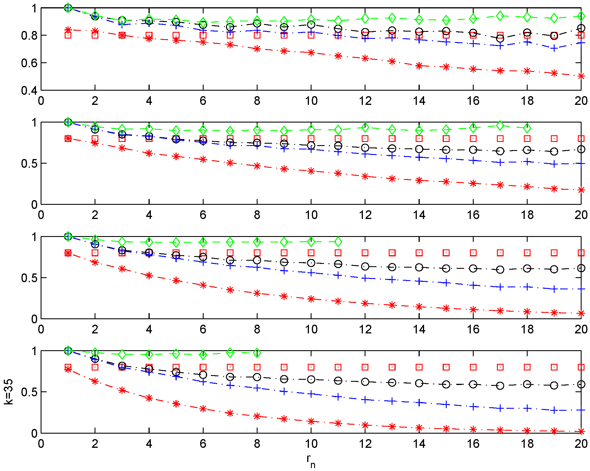
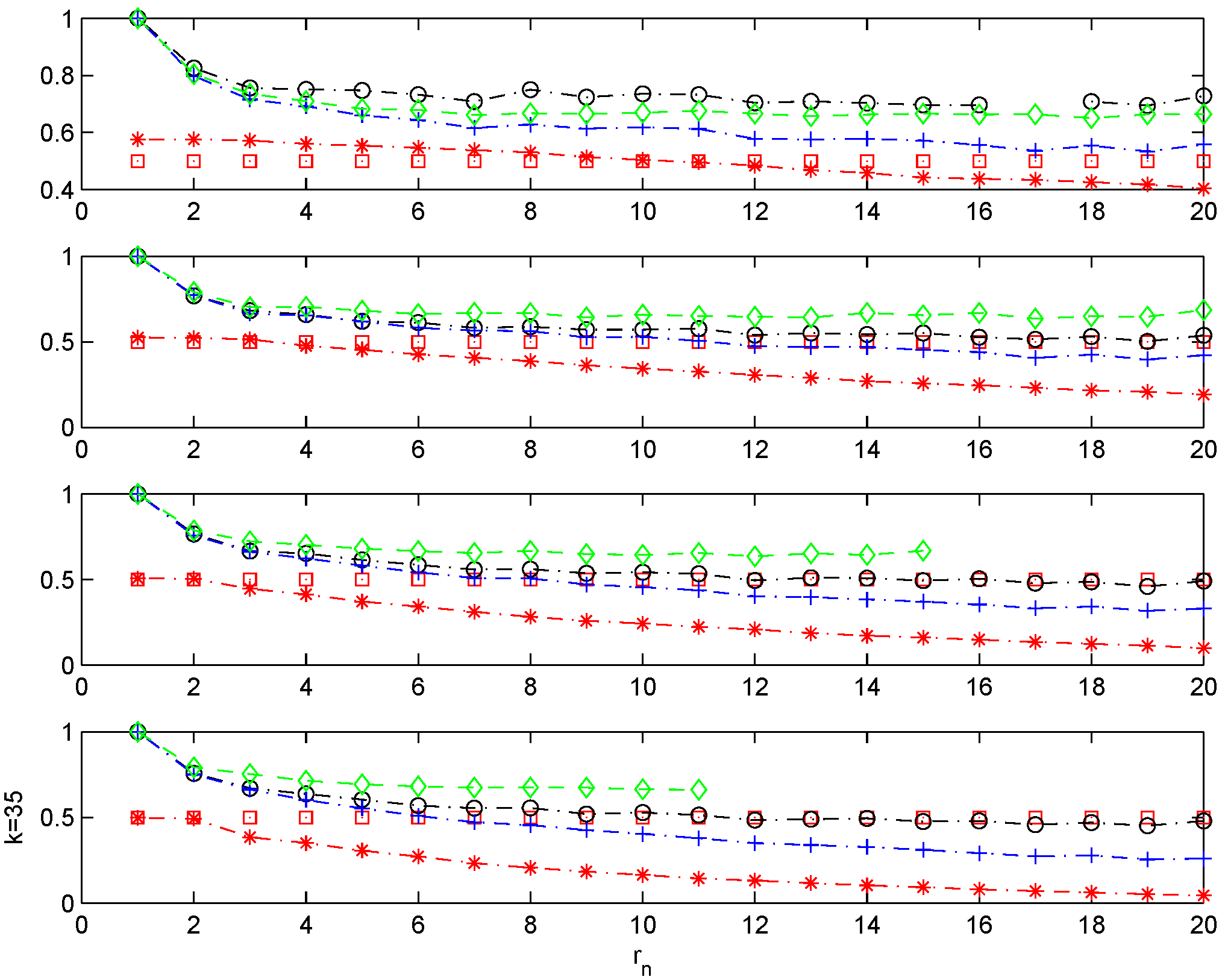
Figure 1 and
Figure 2 report the sequence of estimates of θ for
and
, respectively. The different panels in these figures report the estimates of θ obtained from the logs method, blocks method, runs method and the estimator
, for different levels determined by order statistics
and
with
, and
n = 200.
A close inspection of the charts shows that the blocks and the runs method underestimate θ as increases. This is so because these estimators, by construction, have a decreasing numerator as the block size increases. On the other hand, estimates derived from the logs method are very accurate for the higher threshold sequences employed, but unfortunately, as decreases, the estimator exhibits problems due to the fact that every single block contains an exceedance (). In these cases, this estimator is not well defined. In contrast, shows reliable and stable estimates of θ across all threshold levels and partitions employed.
Figure 1.
Chernick model with . . Sample mean for different estimators of θ. Monte Carlo simulations. , and with ; n = 200. . θ plotted with, with , with , with , and with the line.
Figure 1.
Chernick model with . . Sample mean for different estimators of θ. Monte Carlo simulations. , and with ; n = 200. . θ plotted with, with , with , with , and with the line.
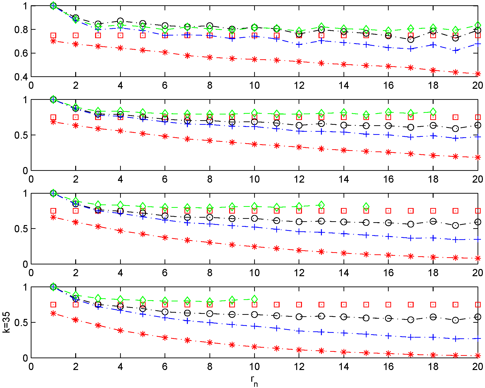
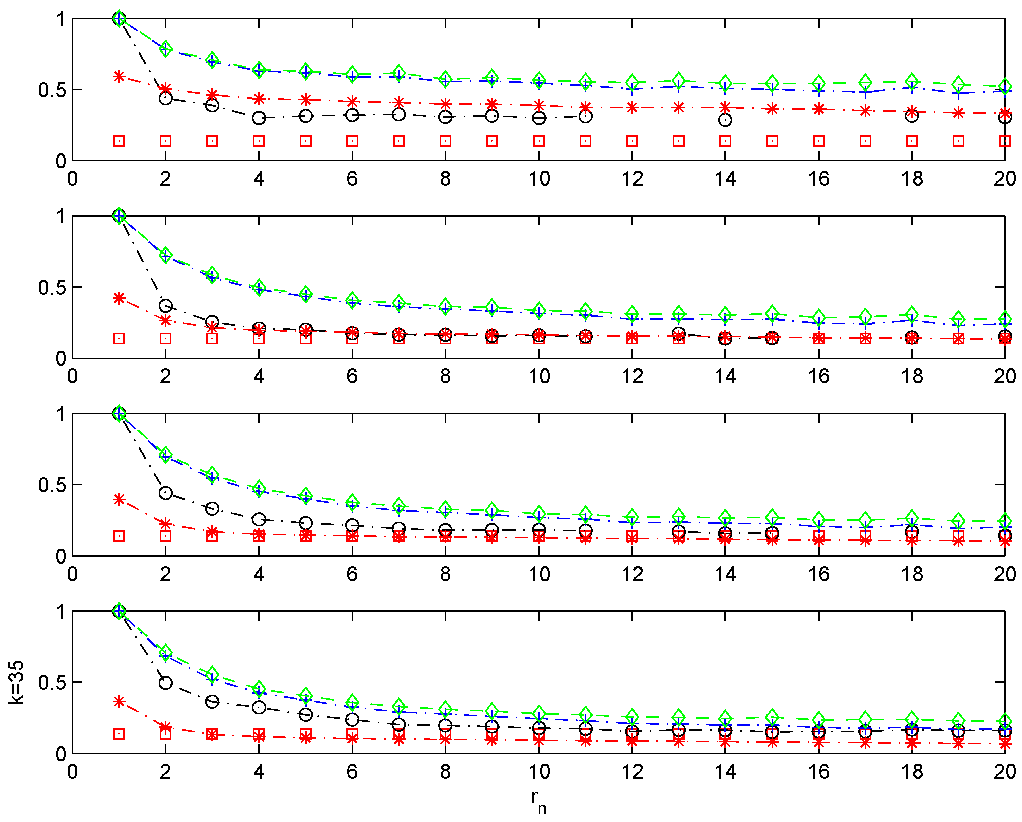
Figure 2.
Chernick model with . .
Figure 2.
Chernick model with . .
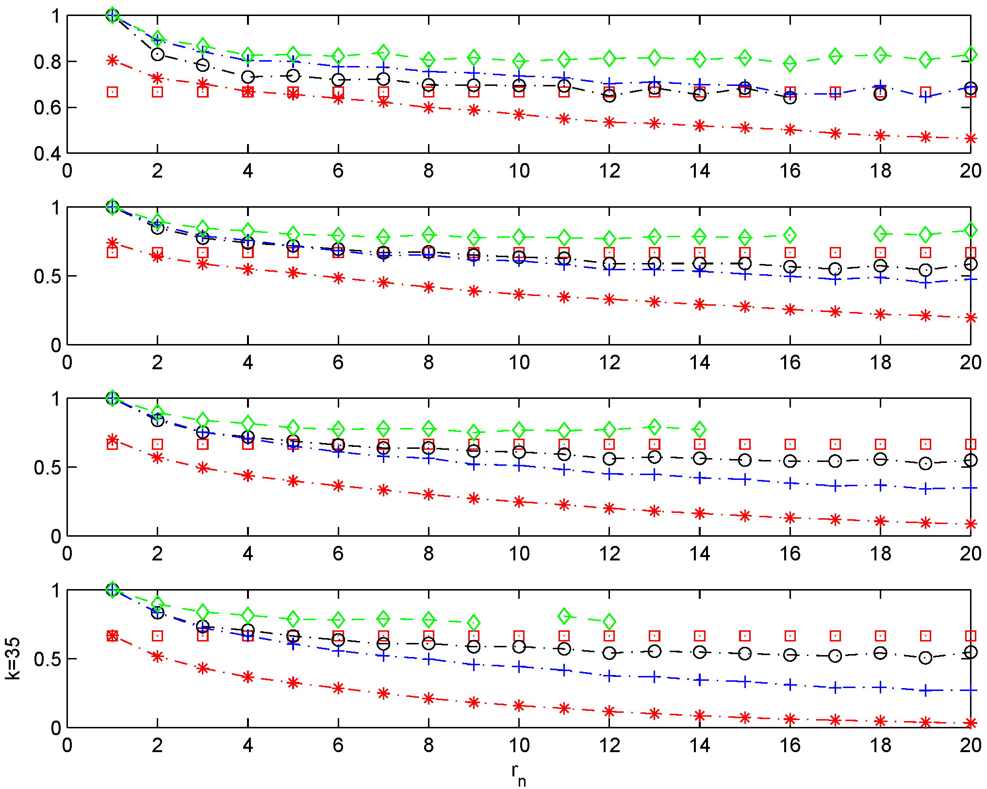
The second process under investigation is the doubly-stochastic model studied in [
4]. Let
be i.i.d. with distribution function
F; suppose that
and for
,
the choice being made independently for each
i. The doubly-stochastic sequence
is defined by
independently of anything else. In this example, the extremal index is
. Smith and Weissman [
4] compare different estimators of θ for
and
(
) and show that the runs method is superior to the rest of the competing estimators.
Figure 3 is consistent with their results.
seems to be, however, a very good competitor of
for every single level and outperforms the logs and blocks estimators across all levels. To compare the performance of the runs method against
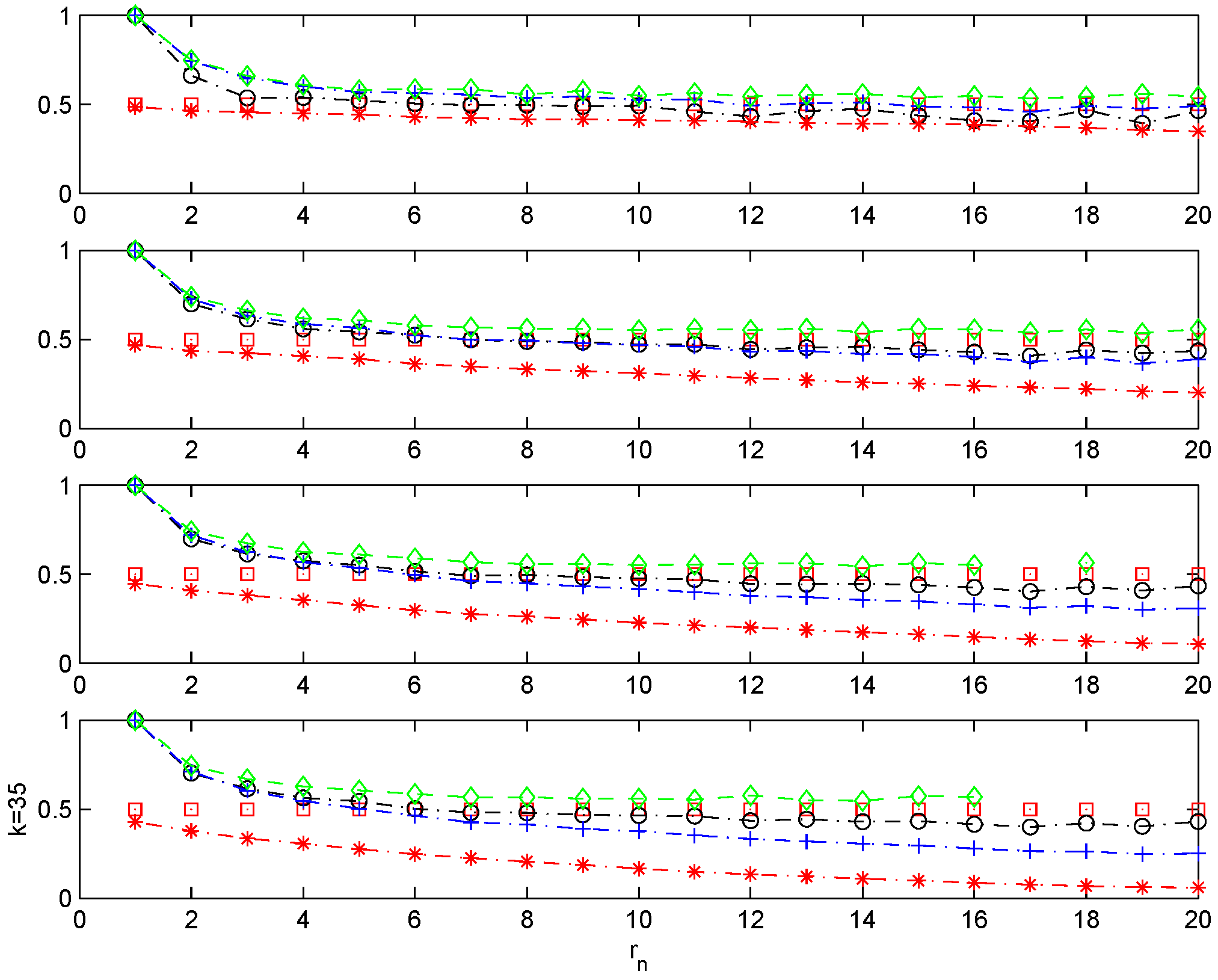
, we also estimate the extremal index of this process for
and
(
). Both of the runs and blocks method exhibit the same declining pattern observed before for increasing block sizes (see
Figure 4). In this case, however,
shows a superior performance to the rest of the estimators. The logs methods is the only competitor exhibiting a similar performance to our family of estimators.
Figure 3.
Doubly-stochastic model with and . . Sample mean for different estimators of θ. Monte Carlo simulations. , and , with ; n = 200. . θ plotted with, with , with , with , and with the line.
Figure 3.
Doubly-stochastic model with and . . Sample mean for different estimators of θ. Monte Carlo simulations. , and , with ; n = 200. . θ plotted with, with , with , with , and with the line.
Figure 4.
Doubly-stochastic model with and . .
Figure 4.
Doubly-stochastic model with and . .
The following example is the moving-maximum process:
, where
is an i.i.d. sequence with the common distribution function standard Fréchet
. The extremal index is
for
and
, otherwise. We consider
.
Figure 5 shows results in the spirit of those found for the Chernick process with
.
This part of the simulation section concludes with the example introduced by L. de Haan:
, where
and
is an i.i.d. sequence with the common distribution function standard Fréchet
. The extremal index is
. The results reported in
Figure 6 for
are consistent with models exhibiting low, but significant clustering; see, for example, the results of the simulation exercise for the Chernick model and
r = 5, where
, and the doubly-stochastic process with
and
, where
.
Figure 5.
Moving-maximum process with . . Sample mean for different estimators of θ. Monte Carlo simulations. , and , with ; n = 200. . θ plotted with, with , with , with , and with the line.
Figure 5.
Moving-maximum process with . . Sample mean for different estimators of θ. Monte Carlo simulations. , and , with ; n = 200. . θ plotted with, with , with , with , and with the line.
Figure 6.
Maximum of the lagged autoregressive process with . .
Figure 6.
Maximum of the lagged autoregressive process with . .
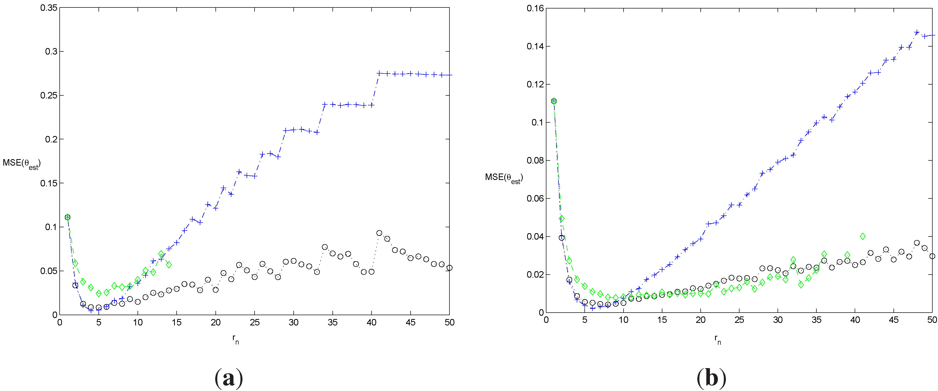
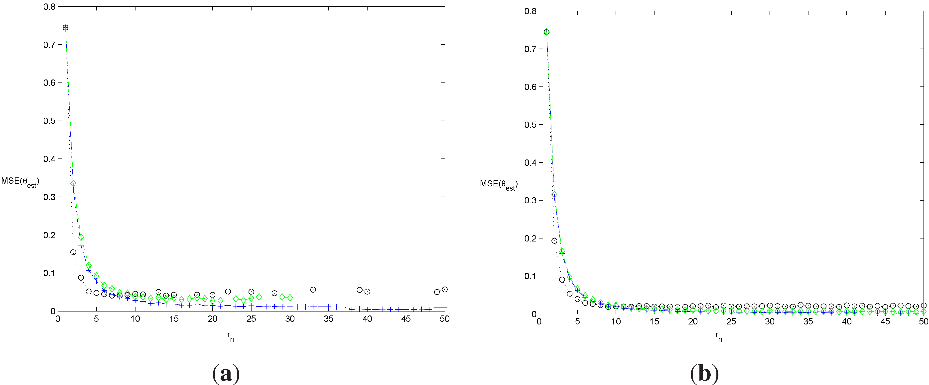
In order to compare the results of the blocks and logs methods with our new feasible estimator more in depth, we report in
Figure 7 and
Figure 8 the estimated mean square error for the doubly-stochastic model. The penalty function is
with
simulated Monte Carlo sequences. The results confirm the findings above. Whereas the blocks method performs rather well for the first simulation experiment, it completely fails to report accurate estimates for the second experiment with a higher extremal index.
Figure 7.
Simulated mean square error (MSE) of the estimators of θ for the doubly-stochastic model with and . Monte Carlo simulations. with , with and with . . n = 200 in (a), and n = 1000 in (b). and with .
Figure 7.
Simulated mean square error (MSE) of the estimators of θ for the doubly-stochastic model with and . Monte Carlo simulations. with , with and with . . n = 200 in (a), and n = 1000 in (b). and with .
Figure 8.
Simulated mean square error (MSE) of the estimators of θ for the doubly-stochastic model with and . Monte Carlo simulations. with , with and with . . n = 200 in (a), and n = 1000 in (b). and with .
Figure 8.
Simulated mean square error (MSE) of the estimators of θ for the doubly-stochastic model with and . Monte Carlo simulations. with , with and with . . n = 200 in (a), and n = 1000 in (b). and with .
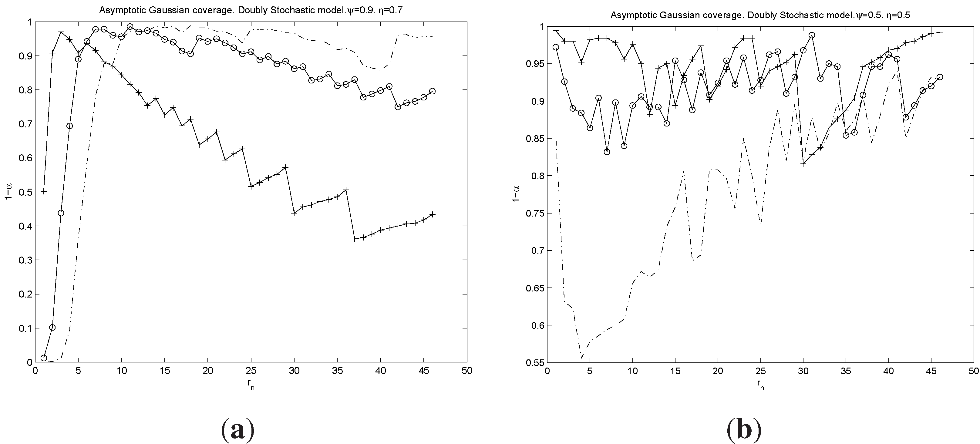
This section concludes with the study of the empirical coverage of the normal distribution followed asymptotically by our family of estimators.
Figure 9 and
Figure 10 report the asymptotic coverage of the two-sided normal confidence intervals for the examples above covering the Chernick and doubly-stochastic models. The simulations are computed for the order statistics above with
and
. The plots illustrate the accuracy of the normal asymptotic distribution in all cases. It is worth noting that the partition of the sample and the extent of clustering play an important role for obtaining the correct nominal coverage for the asymptotic normal approximation. Thus, for large sample sizes, the models exhibiting a low clustering of extremes, Chernick with
and the doubly-stochastic model with
, only provide accurate approximations as the block size increases.
Figure 9.
Chernick model with in (a) and in (b). Monte Carlo simulations. for , for and for . and with , where rounds to the next integer. , . .
Figure 9.
Chernick model with in (a) and in (b). Monte Carlo simulations. for , for and for . and with , where rounds to the next integer. , . .
Figure 10.
Doubly-stochastic model with and and in (a) and in (b). Monte Carlo simulations. for , for and for . and with , where rounds to the next integer. , . .
Figure 10.
Doubly-stochastic model with and and in (a) and in (b). Monte Carlo simulations. for , for and for . and with , where rounds to the next integer. , . .
5. Application to Macroeconomic Time Series
Macroeconomic series usually exhibit clustering of extreme values that indicate periods of crisis, financial distress, booms and bursts. This phenomenon is more acute as the data are studied at shorter frequencies; thus, monthly time series usually exhibit stronger clustering of extremes than quarterly series, and so on. This stylized fact in macroeconomic time series is usually modeled with econometric processes that accommodate volatility clustering; see the ARCH family of volatility processes proposed by [
25] or the stochastic volatility processes developed in [
26]. These processes are, however, silent about the probability of runs of extremes in one or the other tail, and only after tedious calculations, which depend most of the times on a number of parameters, can one compute the chances of these events. Alternatively, inference about the extremal index is an unexplored option in this field that can lead to very interesting insights about the existence of clustering in the extremes of these sequences and on its persistence.
In this application, we pursue this alternative with monthly data in unemployment growth and inflation rates from the United States spanning the period February 1947 until July 2007 for the first series and February 1947 until June 2008 for the second series. Data are obtained from
https://www.economy.com/freelunch. The dynamics of these series are reported in
Figure 11 and
Figure 12. Dickey-Fuller unit root tests reject the null hypothesis, providing statistical support to the stationarity of both series. As pointed out by a referee, the visual inspection of both processes could also suggest the presence of several structural breaks around periods characterized by drastic changes in monetary policy. In this likely scenario, it would also be reasonable to assume that the unemployment growth process and inflation rates are both stationary around a shifting mean, implying that the analysis of the serial dependence of the extremes of both sequences should be carried out separately for each regime. Nevertheless, for simplicity in the description of the problem, we assume hereafter a constant mean in both cases and, in turn, the stationarity of both processes.
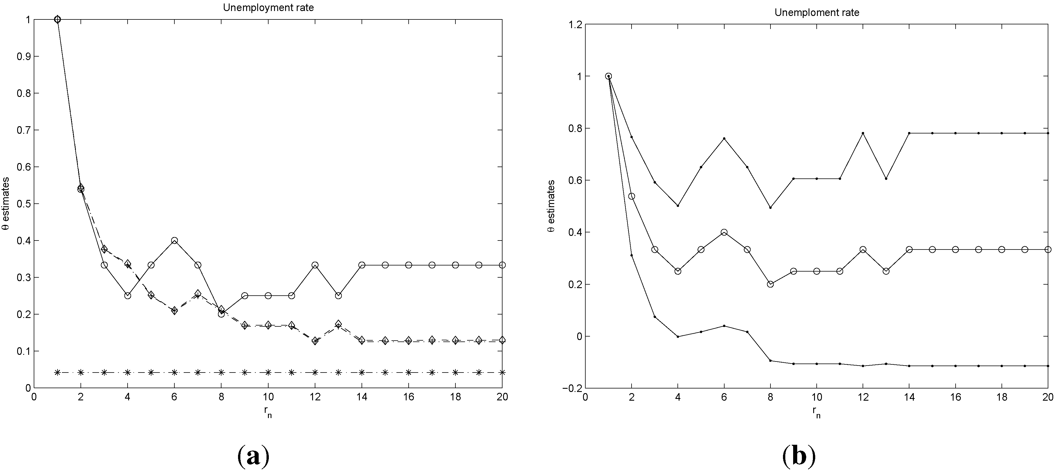
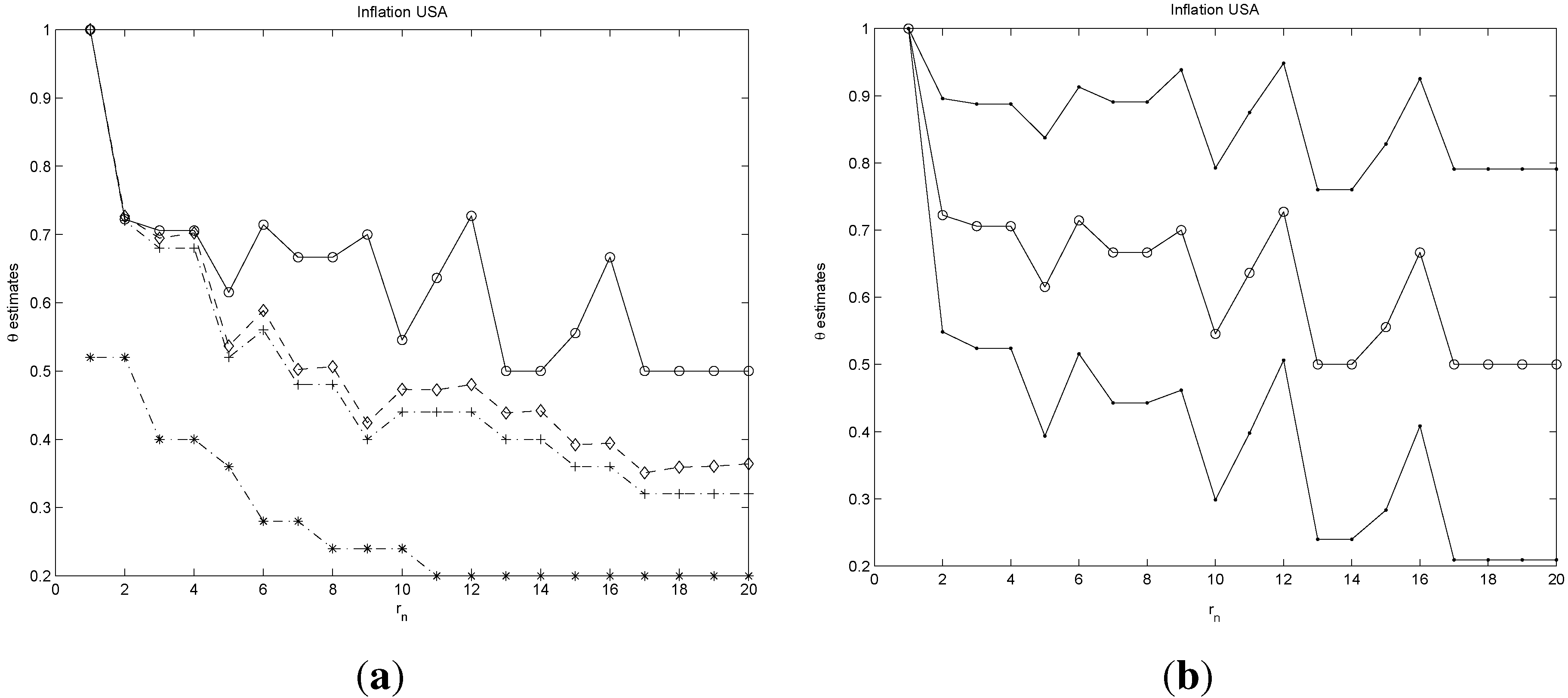
Panel (a) of
Figure 13 and
Figure 14 report the estimates of θ using the four methods discussed in the paper. We can observe from the plots a similar decaying pattern for the four families of estimates. Note, however, that, whereas the sequences of the logs, blocks and runs estimates decay as the block size
increases, the estimator
proposed in this paper stabilizes after the first partitions around a value of 0.3 for unemployment growth and 0.55 for the inflation rate, respectively. The statistical significance of these results is carried out by computing confidence intervals for θ at
using the results of Theorem 2 above. These intervals are displayed on the right panels of
Figure 13 and
Figure 14.
The results on the extremal index point towards a strong clustering in the positive extremes of both sequences. A more detailed analysis obtained by inspecting the confidence levels of each sequence of estimates indicates a stronger clustering for the unemployment series than for inflation.
1 This implies that periods of high unemployment are more persistent than highly inflationary periods. A simple version of the Philips curve (see [
27]) shows that inflation and economic growth are positively correlated or, similarly, that inflation and unemployment are negatively correlated. These empirical observations would imply that high inflation is followed by economic growth and, hence, falls in unemployment. Our empirical analysis of the extremes of both series adds further insights into this relationship. More specifically, we observe that highly inflationary periods are less persistent than periods with large unemployment growth, suggesting that economic policies focused on producing inflation to boost economic growth can only be successful in the very short term, as inflation quickly returns to normal levels. In contrast, large unemployment growth has lingering effects that are not easily reduced by policies aimed at rising inflation.
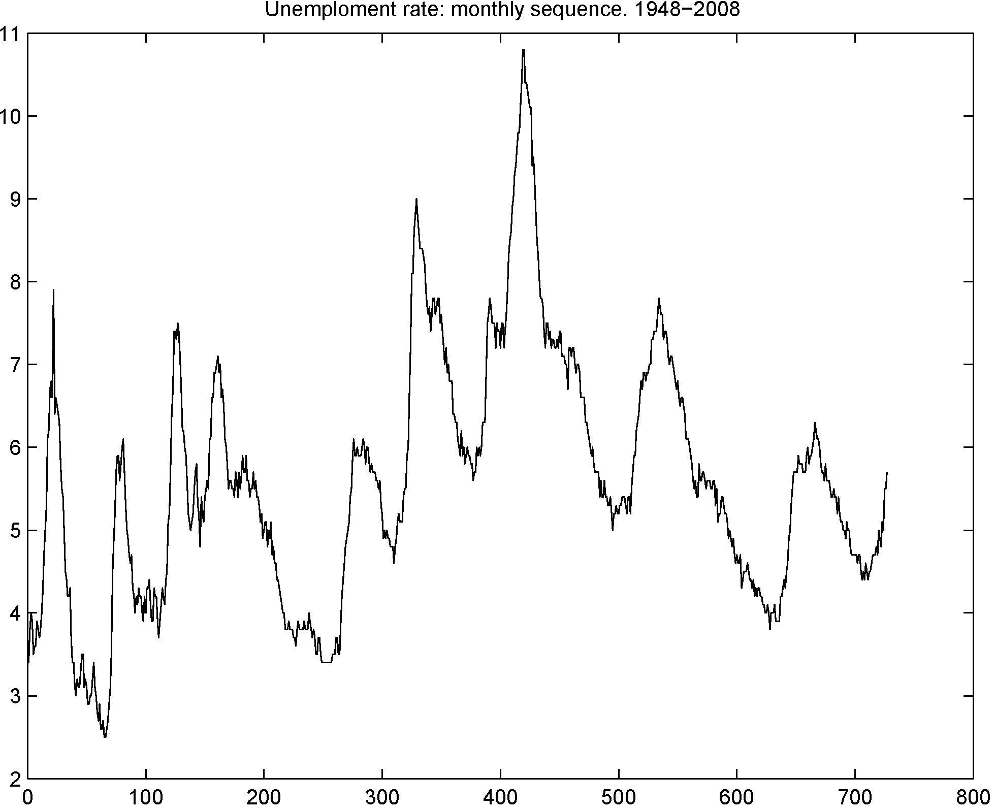
Figure 11.
Monthly time series of unemployment growth for United States spanning the period February 1947 to June 2007.
Figure 11.
Monthly time series of unemployment growth for United States spanning the period February 1947 to June 2007.
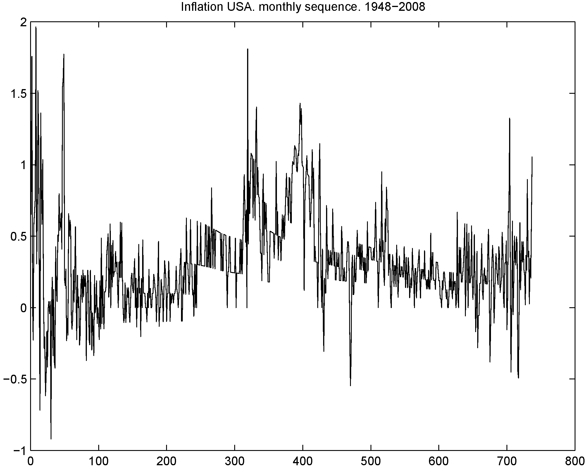
Figure 12.
Monthly time series of inflation rates for the United States spanning the period February 1947 to July 2008.
Figure 12.
Monthly time series of inflation rates for the United States spanning the period February 1947 to July 2008.
Figure 13.
Panel (a) reports different estimates of θ. . with , with , with , and with the line. Panel (b) reports two-sided confidence intervals for θ at computed from , with and , .
Figure 13.
Panel (a) reports different estimates of θ. . with , with , with , and with the line. Panel (b) reports two-sided confidence intervals for θ at computed from , with and , .
Figure 14.
Panel (a) reports different estimates of θ. . with , with , with , and with the line. Panel (b) reports two-sided confidence intervals for θ at computed from , with and , .
Figure 14.
Panel (a) reports different estimates of θ. . with , with , with , and with the line. Panel (b) reports two-sided confidence intervals for θ at computed from , with and , .

