Return and Volatility Spillovers across Equity Markets in Mainland China, Hong Kong and the United States

Abstract

Examinations of the dynamics of daily returns and volatility in stock markets of the U.S., Hong Kong and mainland China (Shanghai and Shenzhen) over 2 January 2001 to 8 February 2013 suggest: (1) evidence of unidirectional return spillovers from the U.S. to the other three markets; but no spillover between Hong Kong and either of the two mainland China markets; (2) evidence of unidirectional ARCH and GARCH effects from the U.S. to the other three markets; (3) correlations of returns vary across markets, with the highest correlation of 93.5% between the two Chinese markets, medium correlation of 30% between mainland China and Hong Kong markets and low correlations of 6.4% and 7.2% between the U.S. and China’s two markets; thus, international investors may benefit by allocating their assets in China’s markets; (4) the patterns of dynamic conditional correlations from the DCC model suggest an increase in correlation between China and other stock markets since the most recent financial crisis of 2007.

1. Introduction

China’s economic reform, which began in the late 1970s, has been accompanied by the development of a modern financial system to allocate financial resources from savers to investors and to attract foreign capital. One important component of such a system is a vibrant and dynamic equity market. China’s current equity market consists of two stock exchanges—the Shanghai Stock Exchange (SSE) and the Shenzhen Stock Exchange (SZSE).

The Shanghai stock exchange was re-established on 26 November 1990 and was in operation on December 19 of the same year. 1 It has become the most preeminent stock market in mainland China and the world’s sixth largest stock exchange by market capitalization at U.S. $2.3 trillion as of December 2011. The Shenzhen stock exchange (SZSE) was established on 1 December 1990 and had a market capitalization of about U.S. $1 trillion in 2011. Both exchanges are subject to tight capital controls and are only partially open to foreign investors. International investors, including residents of Hong Kong, Macau and Taiwan, can participate only in the trading of B shares. 2 The Shanghai Stock Exchange composite index (SH) and Shenzhen Stock Exchange composite index (SZ) are indicators of the performance of mainland China’s stock market.

This study will examine the dynamic relationships among the two stock exchanges of mainland China, Hong Kong and the United States using daily data from 2 January 2001 to 8 February 2013. The primary purpose of the investigation is to explore the possibility of spillovers in return, as well as in conditional volatility across these four markets. The results of this investigation may have important implications regarding international investment, portfolio diversification and risk management.

The Hong Kong Stock Exchange (SEHK) is Asia’s second largest stock exchange in terms of market capitalization and the fifth largest in the world. The Hang Seng index (HK) is a weighted average of equity prices for 48 companies traded in SEHK. It represents about 60% of the capitalization of SEHK and serves as a proxy for its performance. We represent the U.S. equity market by the S&P 500 index (SP), which is based on the market capitalization of 500 leading companies publicly traded in the U.S. stock market.

Several studies have addressed the transmission of return and volatility shocks across equity markets. Earlier studies on the subject have focused on developed markets. King and Wadhwani [1] and Hamao, Masulis and Ng [2] both examine the transmission of volatility across the London, New York and Tokyo markets. Hamao, Masulis and Ng’s [2] application of the ARCH model reveals unidirectional volatility spillovers from New York to London and Tokyo and from London to Tokyo. King and Wadhwani [1] find that the correlation between markets rises following an increase in volatility. Bae and Karolyi [3] investigate spillovers in volatility between Japan and the U.S. using three asymmetric GARCH models (GARCH, PNP-GARCH and GJR-GARCH). 3 Their findings suggest bidirectional relations in volatility between the two markets. Furthermore, bad news tends to have a much larger impact on subsequent return volatility than good news. Karolyi [4] provides additional evidence on the short-run relation between stocks traded in the U.S. and Canada using four alternative models (vector autoregressive (VAR), multivariate generalized autoregressive conditional heteroscedasticity (MGARCH)-BEKK, MGARCH-CCC and the univariate GARCH model). 4

Following the Asian financial crisis of 1997, several studies have explored the possibility of contagion across Asian stock markets. Worthington and Higgs [5] investigate the transmission of stock return and volatility in three Asian developed markets (Hong Kong, Japan and Singapore), as well as six Asian emerging markets (Indonesia, Korea, Malaysia, the Philippines, Taiwan and Thailand). Broadly speaking, their results suggest that all Asian equity markets are highly integrated, though the spillovers are not homogeneous across markets.

More recently, a limited number of studies have explored the potential linkage between stock markets of mainland China and other markets. Poon and Fung [6] examine the relationships among Hong Kong’s H share, red chips and China’s Shanghai and Shenzhen composite indexes. 5 They find significant return transmissions from the red-chip market to the Shenzhen market, from the Shenzhen market to the Shanghai market and from the Shanghai market to the H-share market. They also find volatility spillovers from the red-chip market to the other markets. Joshi [7] examines the return and volatility spillovers among Hong Kong, China and four other Asian stock markets (India, Japan, Indonesia and Korea). His results suggest bidirectional return spillovers between mainland China and Indonesia and bidirectional volatility spillovers between China and each of Japan, Korea and Indonesia.

Although stock market integration has been widely studied, research on the international linkages of the Chinese stock exchanges is rather limited. Bailey [8] is one of the earliest studies on the relationship between China and international stock markets. However, the results of his investigation reveal that return on China’s B shares has little or no correlation with international equity returns. Wang and Firth [9] investigate the correlation of return and volatility between Greater China’s four stock markets (two mainland China’s exchanges, Hong Kong and Taipei) and three major international financial markets (Tokyo, London and New York stock exchanges). Their results suggest that the returns in mainland China’s two stock markets are influenced mostly by the regional developed markets (Hong Kong and Taipei). They also find that mainland China equity markets are relatively segregated. Li [10] examines the relationship among the stock markets of mainland China, Hong Kong and the U.S. His findings also indicate a unidirectional volatility spillover from Hong Kong to mainland China, but no direct linkage between mainland China and the U.S. market. Lucey and Zhang [11] investigate the role of cultural distance on the integration of financial markets. 6 Their examination of 46 stock markets suggests that country pairs tend to exhibit higher linkages if they have smaller cultural distance.

The prevailing evidence from previous studies suggests that China’s stock markets have been fairly isolated from global markets since their establishment. However, the degree of stock market integration has changed over time. Following the 1997 Asian financial crisis, the two markets have become more integrated with local emerging and developed stock markets, but the integration with Western stock markets has remained weak.

This study reexamines the short-run relationships in return and volatility among the equity markets of the U.S., Hong Kong and the two mainland China (Shanghai and Shenzhen). We use a VAR model to explore the causal relations among the returns of these four markets. To examine the possibility of volatility spillovers, we use three alternative multivariate generalized autoregressive conditional heteroscedasticity (MGARCH) models: the BEKK model of Engle and Kroner [13], the constant conditional correlation (CCC) model of Bollerslev [14] and the dynamic conditional correlation model of Engle [15]. Our study makes three contributions to the existing literature: First, it investigates the relationship among these markets using the longest available sample period, which covers 2 January 2001 to 8 February 2013. Second, to allow for a comparison of returns and risks across markets, it adjusts the stock returns to reflect changes in the exchange rate for each country. This is a useful exercise for an international investor who is concerned with portfolio diversification. Third, it investigates the possibility of volatility spillovers using three alternative MGARCH models—the BEKK, the CCC and DCC models. Thus, it allows for a richer set of dynamics among stock returns. The BEKK model is very popular in the previous studies related to China [5,7,10]. However, it is not parsimonious, as it requires the estimation of too many parameters. The CCC and DCC models contain fewer parameters; and the DCC model allows time-varying correlations. However, no previous study has applied these two models to Chinese data.

The results of our investigation can be summarized as follows: (1) the VAR findings suggest unidirectional spillovers in returns from the U.S. to the other three markets, but a lack of spillovers between mainland China and Hong Kong; (2) evidence of unidirectional ARCH and GARCH spillovers in volatility from the U.S. to the other three markets using the BEKK model; (3) evidence from the CCC model suggesting that mainland China’s two stock markets are highly correlated, with an average correlation of 93.5%. The correlations between mainland China’s two markets and the Hong Kong market remain around 30%, while the correlations between mainland China’s two markets and the U.S. are still low, with averages of 6.4% and 7.2%, respectively. Thus, international investors can benefit from diversification by allocating their assets in China’s equity markets. (4) The patterns of the dynamic conditional correlations from the DCC model suggest an increase in correlation between China and the other stock markets since the most recent financial crisis of 2007.

The remainder of this paper is organized as follows: Section 2 addresses the empirical methodology and introduces the VAR and the three MGARCH models used in the investigation. Section 3 presents the data along with their descriptive statistics. Section 4 reports the estimation results, and Section 5 concludes.

2. Models

2.1. Vector Autoregressive (VAR) Model

We examine the possibility of spillovers in returns over time and across markets using a four-variable vector autoregressive (VAR) model consisting of returns for Shanghai, Shenzhen, Hong Kong and the S&P 500 as follow:

$$\begin{array}{l}{R}_t={\mathrm{\Phi }}_0+{\mathrm{\Phi }}_1{R}_{t-1}+\mathrm{...}+{\mathrm{\Phi }}_p{R}_{t-p}+{\epsilon }_t\\ {\epsilon }_t|{\mathrm{\Omega }}_{t-1}~N(0,H_t)\end{array}$$

(1)

where R_t is a four-variable vector of returns in the four markets (SH, SZ, HK, SP) at time t; p is the lag length; Φ₀ is a 4 × 1 vector of intercepts; Φ₁ through Φ_p are coefficient matrices, with their elements capturing their own, as well as the cross-market lag effects; and ε_t is a 4 × 1 vector of error terms. We assume that elements of ε_t are serially uncorrelated, with the conditional variance-covariance matrix represented by the 4 × 4 matrix H_t given the information set Ω_t−1.

According to Equation (1), the return in each market is a linear function of its own past, as well as past returns in the other markets. For example, the return on the Shanghai market (SH) depends on p lags of itself, as well as p lags of the other three returns:

$$R_{1.t}={\varphi }_1+{\displaystyle \sum _{i=1}^p{\phi }_{1i}{R}_{1,t-i}}+{\displaystyle \sum _{i=1}^p{\phi }_{2i}{R}_{2,t-i}}+{\displaystyle \sum _{i=1}^p{\phi }_{3i}{R}_{3,t-i}}{\displaystyle \sum _{i=1}^p{\phi }_{4i}{R}_{4,t-i}+}{\epsilon }_{1,t}$$

(2)

The possibility of spillover in returns over time can be examined by testing the joint hypotheses that φ_1i = 0 (i = 1, …, p). Similarly, the possibility of spillovers in returns from Market 2 to Market 1 can be examined by testing for the joint hypotheses that φ_2i = 0 (i = 1, …, p).

2.2. Multivariate GARCH Models

We explore the temporal dependence of the conditional variance, H_t, using three alternative multivariate generalized autoregressive conditional heteroscedasticity (MGARCH) models: The BEKK model of Engle and Kroner [13], the constant conditional correlation (CCC) model of Bollerslev [14] and the dynamic conditional correlation (DCC) model of Engle [15].

2.2.1. MGARCH-BEKK

The BEKK model of Engle and Kroner [13] can be written as,

$$H_t=C\prime C+{\displaystyle \sum _{i=1}^k{A}_i^{\prime }}{\epsilon }_{t-i}{\epsilon }_{t-i}^{\prime }{A}_i+{\displaystyle \sum _{i=1}^k{G}_i^{\prime }}{H}_{t-i}{G}_i$$

(3)

where C, A_i and G_i are N × N matrices, but C is triangular. This equation guarantees all positive definite diagonal representations. In the analysis that follows, we will set the lag length to one, which results in a parsimonious specification of the BEKK model as,

$$H_t=C\prime C+A\prime {\epsilon }_{t-1}{\epsilon }_{t-1}^{\prime }A+G\prime H_{t-1}G$$

(4)

The BEKK model provides a convenient way of decomposing each conditional variance into its ARCH and GARCH components. For example, the ARCH component associated with the conditional variance of Shanghai (SH) can be written as:

$$\begin{array}{l}{h}_{11,t}=c_1+a_{11}^2{\mathrm{\epsilon }}_{1,t-1}^2+a_{21}^2{\mathrm{\epsilon }}_{2,t-1}^2+a_{31}^2{\mathrm{\epsilon }}_{3,t-1}^2+a_{41}^2{\mathrm{\epsilon }}_{4,t-1}^2\\ +2a_{11}{a}_{21}{\mathrm{\epsilon }}_{1,t-1}{\mathrm{\epsilon }}_{2,t-1}+2a_{11}{a}_{31}{\mathrm{\epsilon }}_{1,t-1}{\mathrm{\epsilon }}_{3,t-1}+2a_{11}{a}_{41}{\mathrm{\epsilon }}_{1,t-1}{\mathrm{\epsilon }}_{4,t-1}\\ +2a_{21}{a}_{31}{\mathrm{\epsilon }}_{2,t-1}{\mathrm{\epsilon }}_{3,t-1}+2a_{21}{a}_{41}{\mathrm{\epsilon }}_{2,t-1}{\mathrm{\epsilon }}_{4,t-1}+2a_{31}{a}_{41}{\mathrm{\epsilon }}_{3,t-1}{\mathrm{\epsilon }}_{4,t-1}\end{array}$$

where the ARCH volatility in the SH return depends on the squares, as well as the cross-products of the previous period shocks associated with the four markets. Here, a₁₁, a₂₁, a₃₁, a₄₁ capture the effects of past squared shocks in each market on today’ volatility in SH returns.

Similarly, the GARCH component of the Shanghai (SH) conditional variance can be written as,

$$\begin{array}{l}{h}_{11,t}=g_{11}^2{h}_{11,t-1}+g_{21}^2{h}_{22,t-1}+g_{31}^2{h}_{33,t-1}+g_{41}^2{h}_{44,t-1}\\ +2g_{11}{g}_{21}{h}_{12,t-1}+2g_{11}{g}_{31}{h}_{13,t-1}+2g_{11}{g}_{41}{h}_{14,t-1}\\ +2g_{21}{g}_{31}{h}_{23,t-1}+2g_{21}{g}_{41}{h}_{24,t-1}+2g_{31}{g}_{41}{h}_{34,t-1}\end{array}$$

where the volatility of SH return depends on the past conditional variances and covariances associated with each of the four markets. Here, g₁₁, g₂₁, g₃₁, g₄₁ capture the effects of past volatility in each of the four markets on today’s volatility in SH.

Although the BEKK model provides a useful framework to analyze cross-market spillovers in volatility, it is not parsimonious and requires the estimation of a large set of parameters [16]. The alternative CCC model of Bollerslev [14] and the DCC model of Engle [15] provide more parsimonious specifications.

2.2.2. MGARCH-CCC

The MGARCH-CCC model of Bollerslev [14] allows for time-varying conditional variances and covariances, but restricts the conditional correlations to be constant. The conditional variance matrix is defined as,

$$H_t=D_{t}R{D}_t=({\rho }_{ij}\sqrt{h_{iit}{h}_{jjt}})$$

(5)

where D_t denotes the 4 × 4 stochastic diagonal matrix with elements σ_1t, σ_2t, σ_3t, σ_4t, and R is a 4 × 4 time invariant correlation matrix.

A GARCH (1,1) specification of each conditional variance can be written as,

$$\begin{array}{l}{h}_{iit}=c_i+a_i{\mathrm{\epsilon }}_{i,t-1}^2+g_i{h}_{ii,t-1}\\ h_{ijt}={\mathrm{\rho }}_{ij}\sqrt{h_{iit}{h}_{jjt}};i,j=1,\mathrm{...},4.\end{array}$$

The CCC model parameterizes each conditional variance as a linear function of its own past squared shocks and past conditional variance. It also allows for constant conditional correlations between each pair of markets. Thus, it produces a parsimonious model by reducing the number of unknown parameters.

2.2.3. MGARCH-DCC

There are some indications that the degree of stock market integration has been changing over time (see, for example: [17,18]). Thus, the assumption of constant conditional correlation may not seem realistic. Tse and Tsui [19] and Engle [15] have proposed alternative dynamic conditional correlation (DCC) models, where the conditional correlation is allowed to vary over time. This paper adopts the DCC model of Engle [15],

$$H_t=D_t{R}_t{D}_t$$

where the conditional correlation matrix, R_t, is time varying and is defined as:

$$R_t=diag(q_{11,t}^{-1/2}\mathrm{...}{q}_{44,t}^{-1/2})Q_{t}diag(q_{11,t}^{-1/2}\mathrm{...}{q}_{44,t}^{-1/2})$$

where the 4 × 4 symmetric positive definite matrix $Q_t=(q_{ij,t})$ is given by:

$$Q_t=(1-\alpha -\beta )\overline{Q}+\alpha {\epsilon }_{t-1}{\epsilon }_{t-1}^{\prime }+\beta Q_{t-1}$$

where Q_t is the conditional covariance matrix of the error terms, $\overline{Q}$ is the unconditional covariance matrix and α and β are non-negative scalar parameters with the restriction that α + β < 1. If α = β = 0, then Q_t is equal to $\overline{Q}$, and the constant conditional correlation model will be enough to estimate the correlation matrix. The value of α + β close to one indicates high persistence in the conditional variance.

3. Data

The empirical work in this study requires daily data on stock prices for the Shanghai Stock Exchange (SSE), Shenzhen Stock Exchange (SZSE), Hong Kong Stock Exchange (SEHK) and the U.S. Stock Exchange (U.S.). We measure prices in SSE by its composite index, for SZSE by its composite index, for SEHK by the Hang Seng index and for the U.S. by the S&P 500 index. The close-of-the-day index prices cover the period from 2 January 2001 to 8 February 2013. All prices are adjusted for dividends and splits. Due to holidays, the stock markets in China and the U.S. might be closed on different days. To address this, Wang and Firth [9] and Li [10] omit all observations with missing values. We address the missing values by replacing them with values from the prior day when the market was open. Following this adjustment, there are a total of 3159 daily observations.

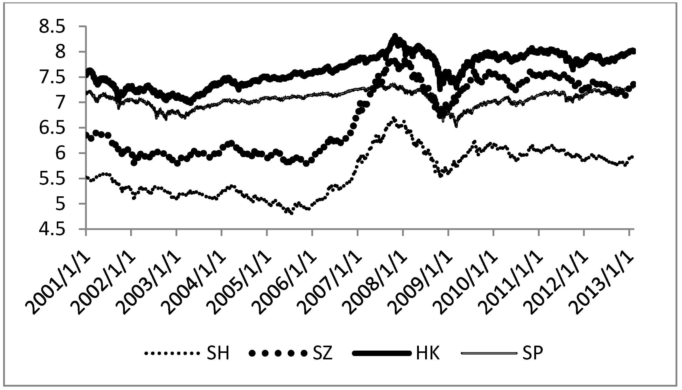
The empirical analysis that follows requires variables that are: (a) in the same units of currency; and (b) stationary. 7 We address the former by converting all price indexes to the U.S dollar using the corresponding exchange rates. Figure 1 shows the plots of these stock indexes after conversion.

Figure 1. Plots of stock prices in logarithms. SH, Shanghai Stock Exchange composite index; SZ, Shenzhen Stock Exchange composite index; HK, Hang Seng index; SP, S&P 500 index.

Figure 1. Plots of stock prices in logarithms. SH, Shanghai Stock Exchange composite index; SZ, Shenzhen Stock Exchange composite index; HK, Hang Seng index; SP, S&P 500 index.

As for the latter, we formally test for unit roots in each stock index using the augmented Dickey-Fuller test. The results (available upon request) suggest that all log prices are non-stationary in level, but stationary in first-difference. Thus, we work with daily returns, which are obtained as the first difference of the natural logarithm of the closing prices for the two consecutive trading days,

$$R_{i,t}=[\log (P_{i,t})-\log (P_{i,t-1})]\times 100$$

Figure 2 presents the daily rates of return for the four adjusted indexes. Daily returns fluctuate around zero and are characterized by volatility clustering. All returns demonstrate higher volatility in 2001–2002, and 2007–2009. However, the two Chinese markets (SH and SZ) appear more volatile.

Figure 2. Daily rates of return in the four stock indices.

Figure 2. Daily rates of return in the four stock indices.

Table 1 reports the summary of statistics for the return series. Three patterns are evident from the table: (1) Average daily returns are positive across the four markets. The daily returns of SH and SZ are larger than the daily returns of HK and SP. This is more evident in the annualized rates of return reported in Row 2. The SZ index has the largest annual rate of return of 12.4%, followed by SH and HK with annualized returns of 5.3% and 5.2%, respectively. SP has the smallest annual return, with a value of 1.6%. (2) The four markets exhibit similar degrees of volatility, as reflected in their standard deviations. The standard deviations are between 1.3% and 1.8%. SZ has the largest standard deviation; SH and HK are about the same; SP is the least volatile series. (3) All series, except for HK, have small negative skewness. The negative skewness in SH, SZ and SP implies that large negative changes in returns occur more often than positive changes. All return series display excess kurtosis. The excess kurtosis in a series implies that large changes occur more often than would be the case if the series had a normal distribution. This is also confirmed by the large Jarque-Bera statistics, which reject the null hypothesis of normal distribution for all series. Finally, the Ljung-Box Q test rejects the null hypothesis of serial independence for each return; the McLeod-Li test rejects the null hypothesis of serial independence in squares of each return series; and the ARCH test rejects the null hypothesis of conditional homoscedasticity.

Table 1. Summary statistics on rates of returns on Shanghai, Shenzhen, Hong Kong and S&P 500.

Statistics	SH	SZ	HK	SP
Mean	0.0001	0.0003	0.0001	0.0000
Mean (annualized)	0.053	0.124	0.052	0.016
Median	0.0000	0.0000	0.0000	0.0003
Maximum	0.0940	0.0976	0.1340	0.1096
Minimum	−0.0915	−0.0964	−0.1359	−0.0947
SD	0.0160	0.0178	0.0155	0.0132
Skewness	−0.0995	−0.1116	0.0044	−0.1771
Kurtosis	7.3845	6.7037	11.8919	11.3451
Jarque-Bera	2530.769	1808.690	10,378.370	9165.545
Probability	(0.00) *	(0.00) *	(0.00) *	(0.00) *
Q(40)	83.71 (0.00) *	83.01 (0.00) *	99.91 (0.00) *	124.91 (0.00) *
QS(40)	968.36 (0.00) *	1006.70 (0.00) *	4203.50 (0.00) *	6601.01 (0.00) *
ARCH(20)	12.74 (0.00) *	13.98 (0.00) *	60.05 (0.00) *	70.19 (0.00) *

Notes. SH, SZ, HK and SP are daily returns on Shanghai, Shenzhen, Hong Kong stock exchanges and the S&P 500 index, respectively. Q(40), QS(40) are Ljung-Box and McLeod-Li tests of serial correlation of up to 40th order in the level and squares of returns. ARCH(20) is a test of conditional heteroscedasticity of 20th order. * Significant at 5% or better.

Table 1. Summary statistics on rates of returns on Shanghai, Shenzhen, Hong Kong and S&P 500.

Statistics	SH	SZ	HK	SP
Mean	0.0001	0.0003	0.0001	0.0000
Mean (annualized)	0.053	0.124	0.052	0.016
Median	0.0000	0.0000	0.0000	0.0003
Maximum	0.0940	0.0976	0.1340	0.1096
Minimum	−0.0915	−0.0964	−0.1359	−0.0947
SD	0.0160	0.0178	0.0155	0.0132
Skewness	−0.0995	−0.1116	0.0044	−0.1771
Kurtosis	7.3845	6.7037	11.8919	11.3451
Jarque-Bera	2530.769	1808.690	10,378.370	9165.545
Probability	(0.00) *	(0.00) *	(0.00) *	(0.00) *
Q(40)	83.71 (0.00) *	83.01 (0.00) *	99.91 (0.00) *	124.91 (0.00) *
QS(40)	968.36 (0.00) *	1006.70 (0.00) *	4203.50 (0.00) *	6601.01 (0.00) *
ARCH(20)	12.74 (0.00) *	13.98 (0.00) *	60.05 (0.00) *	70.19 (0.00) *

Notes. SH, SZ, HK and SP are daily returns on Shanghai, Shenzhen, Hong Kong stock exchanges and the S&P 500 index, respectively. Q(40), QS(40) are Ljung-Box and McLeod-Li tests of serial correlation of up to 40th order in the level and squares of returns. ARCH(20) is a test of conditional heteroscedasticity of 20th order. * Significant at 5% or better.

4. Results and Discussion

This section reports the results of estimating the VAR-MGARCH models using the returns in the four equity markets. 8 All empirical work is carried out using the RATS 8.0 statistical software.

4.1. VAR Estimation Results

We examine the causal relations among the four stock returns using a VAR(2) model, where the lag length of two is chosen by the Schwarz information criterion. 9 Thus, we regress the daily return in each market on two lags of itself, as well as two lags of returns in each of the three other markets.

Table 2 reports the results of F-statistics on tests of causality among markets (p-values in parentheses). Column 1 reports the response of SH returns to its own lags, as well as lag returns in the other three markets. For example, the F-value of 2.046 in the first cell suggests that past changes in SH return do not have a significant effect on its today’s return. Similarly, the F-value of 1.800 in the second cell suggests that changes in SZ return do not have a significant effect on SH return. Four patterns are evident from this table: (1) all returns depend on their own history, suggesting the existence of their own spillovers over time; the only exception is the return in SH, which is exogenous to its own past changes; (2) all returns are influenced by past returns in SP, but SP returns are not influenced by the returns in any of the other markets; thus, there is evidence of unidirectional spillovers in returns from the SP to other markets; (3) there is no evidence of causality from HK or SZ to any of the other three markets; (4) with respect to the two mainland China markets, there is evidence of unidirectional causality from SH to SZ.

Table 2. F-statistics for tests of causality in return equations in a four-variable vector autoregressive (VAR) model.

	Dependent Variables
	SH	SZ	HK	SP
SH	2.045 (0.130)	7.458 (0.001) *	0.448 (0.639)	0.296 (0.744)
SZ	1.800 (0.166)	7.566 (0.001) *	0.188 (0.828)	0.189 (0.827)
HK	1.108 (0.330)	1.649 (0.192)	36.926 (0.000) *	0.614 (0.541)
SP	28.699 (0.000) *	23.151 (0.000) *	407.392 (0.000) *	15.199 (0.000) *

Notes. Significance levels are in parenthesis. * Indicates significance at the 5% level or better.

Table 2. F-statistics for tests of causality in return equations in a four-variable vector autoregressive (VAR) model.

	Dependent Variables
	SH	SZ	HK	SP
SH	2.045 (0.130)	7.458 (0.001) *	0.448 (0.639)	0.296 (0.744)
SZ	1.800 (0.166)	7.566 (0.001) *	0.188 (0.828)	0.189 (0.827)
HK	1.108 (0.330)	1.649 (0.192)	36.926 (0.000) *	0.614 (0.541)
SP	28.699 (0.000) *	23.151 (0.000) *	407.392 (0.000) *	15.199 (0.000) *

Notes. Significance levels are in parenthesis. * Indicates significance at the 5% level or better.

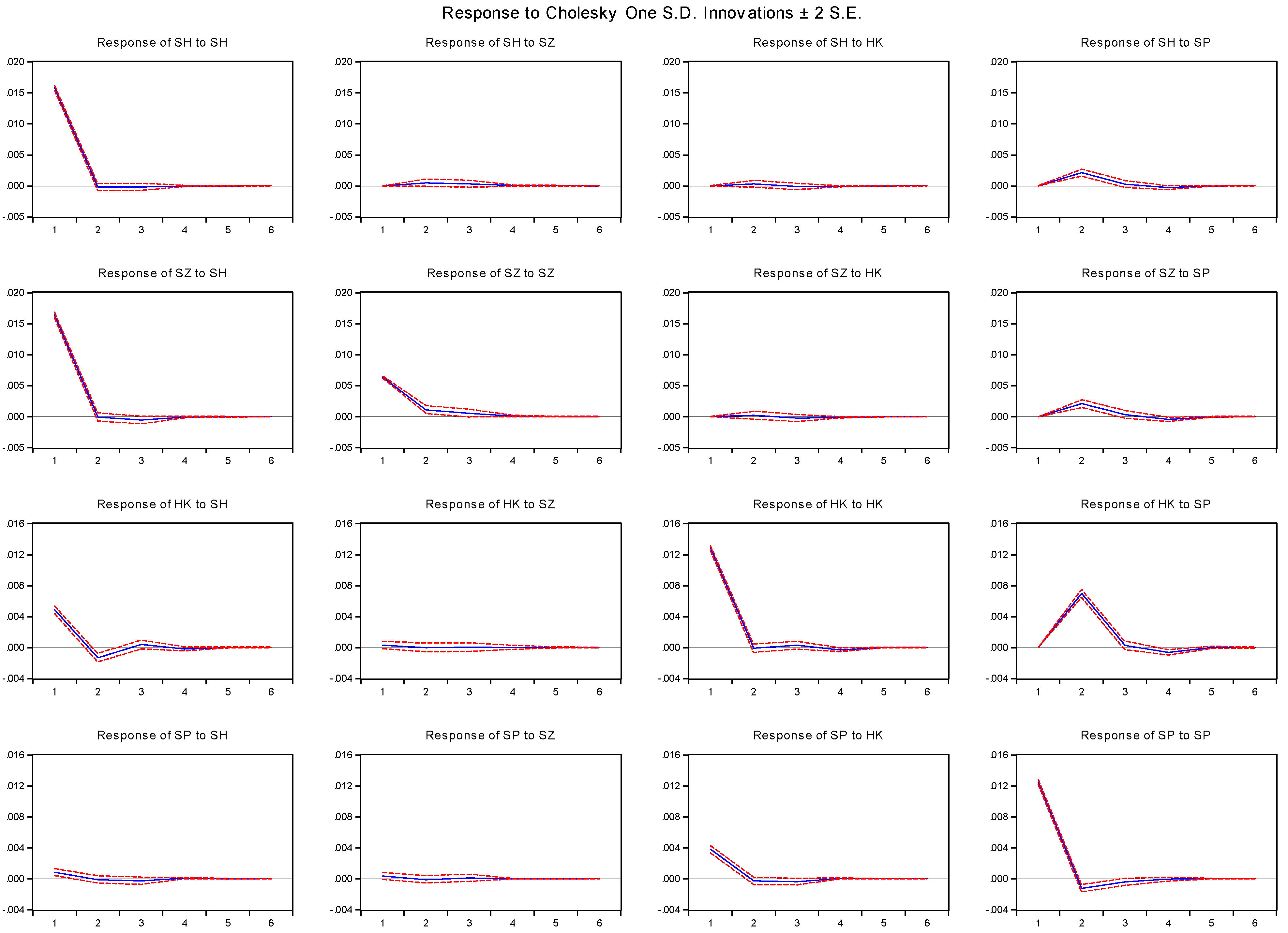
In summary, we find unidirectional return spillovers from SP to the other three markets and also from SH to SZ. This finding is consistent with Wang and Firth [9], but contradicts Li [10], who finds unidirectional return spillovers from Hong Kong to mainland China stock exchanges. 10

Figure 3 plots the impulse response functions of returns to their own shocks, as well as to shocks in other markets along with their 95% confidence bounds. Three patterns of response are evident: First, the response of returns to their own shocks (figures along the diagonal) are positive on the first day, but oscillate and die out after the following days. Second, the responses of SH, SZ and HK to shocks in SP (Column 4) are significantly positive following the shock and die out after two days. This partly reflects the fact that mainland China and Hong Kong markets are at least 12 h ahead of the United States markets. Third, the response of each return series to cross-market innovations varies: (1) each return series responds to shocks in SH (Column 1) and in SP (Column 4); thus, events in Shanghai and the U.S. stock markets have significant effects on returns across all markets; (2) returns do not respond to shocks in SZ (Column 2); (3) returns in mainland China do not respond to shocks in HK, but the response of SP to shocks in HK is positive and significant. Finally, the impulse response functions suggest rapid dissemination of price information across stock exchanges, which is consistent with an efficient operation of the market.

Figure 3. Impulse response functions.

Figure 3. Impulse response functions.

4.2. GARCH-BEKK Results

Next, we examine the patterns of conditional volatility in returns, the possibility of volatility spillovers across markets and the dynamics of conditional correlations in returns across the four stock markets. We begin with the estimation results for the MGARCH-BEKK model, which are reported in Table 3.

Panel A of the table reports the estimates of BEKK parameters. Here, A(. , i) and G(. , i) are the corresponding ARCH and GARCH parameters associated with market i. The squared ARCH parameters [A(. , i)]² capture the responses of volatility in market i to squared standardized innovations in each of the four markets. For example, the estimated ARCH response for SH (i = 1) to its own innovations, [A(1, 1)]², is 0.165², to innovations in SZ is [A(2, 1)]² = (−0.008)², to innovations in HK is [A(3, 1)]² = (0.025)² and to innovations in SP is [A(4, 1)]² = (0.011)². Thus, the volatility of SH responds significantly to past squared shocks in its own market, as well as the Hong Kong stock market.

Table 3. Estimates of ARCH and GARCH parameters in the BEKK model.

Dependent Variables
Panel A. Parameter Estimates
Parameters	SH(. , 1)	SZ(. , 2)	HK(. , 3)	SP(. , 4)
C(i, i)	0.001 (0.000) *	0.001 (0.000) *	0.000 (0.000)	0.000 (0.002)
A(1, .)	0.165 (0.029) *	−0.034 (0.038)	0.043 (0.022)	−0.015 (0.020)
A(2, .)	−0.008 (0.030)	0.241 (0.037) *	−0.027 (0.023)	0.009 (0.020)
A(3, .)	0.025 (0.012) *	0.003 (0.014)	0.185 (0.012) *	−0.023 (0.014)
A(4, .)	0.011 (0.012)	0.010 (0.014)	0.046 (0.016) *	0.265 (0.012) *
G(1, .)	0.998 (0.008) *	0.033 (0.010) *	−0.009 (0.007)	0.001 (0.007)
G(2, .)	−0.012 (0.008)	0.945 (0.010) *	0.007 (0.008)	0.002 (0.007)
G(3, .)	−0.006 (0.003) *	−0.002 (0.004)	0.978 (0.003) *	0.003 (0.003)
G(4, .)	−0.004 (0.003)	−0.005 (0.004)	−0.010 (0.005) *	0.960 (0.003) *
Panel B. Diagnostic Tests
Q(40)	64.129 (0.009) *	66.316 (0.006) *	64.950 (0.008) *	46.805 (0.213)
QS(40)	46.872 (0.211)	41.573 (0.402)	43.955 (0.308)	62.344 (0.013) *

Notes. A(. , i) and G(. , i) are the corresponding ARCH and GARCH parameters for market i. Q(40) is the Ljung-Box test of serial correlation of up to 40th order in standardized residuals. QS(40) is the McLeod-Li test of serial correlation of up to 40th order in the squares of standardized residuals. * Significant at 5% or better.

Table 3. Estimates of ARCH and GARCH parameters in the BEKK model.

Dependent Variables
Panel A. Parameter Estimates
Parameters	SH(. , 1)	SZ(. , 2)	HK(. , 3)	SP(. , 4)
C(i, i)	0.001 (0.000) *	0.001 (0.000) *	0.000 (0.000)	0.000 (0.002)
A(1, .)	0.165 (0.029) *	−0.034 (0.038)	0.043 (0.022)	−0.015 (0.020)
A(2, .)	−0.008 (0.030)	0.241 (0.037) *	−0.027 (0.023)	0.009 (0.020)
A(3, .)	0.025 (0.012) *	0.003 (0.014)	0.185 (0.012) *	−0.023 (0.014)
A(4, .)	0.011 (0.012)	0.010 (0.014)	0.046 (0.016) *	0.265 (0.012) *
G(1, .)	0.998 (0.008) *	0.033 (0.010) *	−0.009 (0.007)	0.001 (0.007)
G(2, .)	−0.012 (0.008)	0.945 (0.010) *	0.007 (0.008)	0.002 (0.007)
G(3, .)	−0.006 (0.003) *	−0.002 (0.004)	0.978 (0.003) *	0.003 (0.003)
G(4, .)	−0.004 (0.003)	−0.005 (0.004)	−0.010 (0.005) *	0.960 (0.003) *
Panel B. Diagnostic Tests
Q(40)	64.129 (0.009) *	66.316 (0.006) *	64.950 (0.008) *	46.805 (0.213)
QS(40)	46.872 (0.211)	41.573 (0.402)	43.955 (0.308)	62.344 (0.013) *

Notes. A(. , i) and G(. , i) are the corresponding ARCH and GARCH parameters for market i. Q(40) is the Ljung-Box test of serial correlation of up to 40th order in standardized residuals. QS(40) is the McLeod-Li test of serial correlation of up to 40th order in the squares of standardized residuals. * Significant at 5% or better.

The ARCH effects demonstrate four unique patterns: (1) All diagonal elements A(1, 1), A(2, 2), A(3, 3) and A(4, 4) are statistically significant, suggesting that each conditional variance depends on its own squared lagged innovations. The SP has the largest own ARCH effect with the coefficient value of 0.265², while SH has the smallest own ARCH effect with the value of 0.165². (2) Past shocks in the U.S. stock market do not affect the variances of the two mainland China markets, while they do have influence on the Hong Kong stock market. (3) There is evidence of a unidirectional ARCH effect from Hong Kong to Shanghai, as reflected in the coefficient of A(3, 1) in Column 1. Shenzhen is the most isolated market. Past shocks in the Shenzhen market have no effect on the volatility of the other markets, and past shocks in any of the other three markets do not affect the volatility of the Shenzhen market.

Similarly, the squared GARCH parameters G(. , i) capture the responses of volatility in market i to past volatility in each of the four markets. For example, the estimated GARCH response for SH (i = 1) to its own past volatility is [G(1, 1)]² = 0.998², to volatility in SZ is [G(2, 1)] = (−0.011)², to volatility in HK is [G(3, 1)] = (−0.006)² and to volatility in SP is [G(4, 1)] = (−0.004)². Again, SH responds significantly to past volatility in the Hong Kong stock market, as well as its own market.

The GARCH effects reveal three patterns: (1) All four conditional variances depend on their own history; this is evident in the estimated G(1, 1), G(2, 2), G(3, 3) and G(4, 4) GARCH parameters, which are all significant at the 5% level. The results also show that own spillovers are always much larger than the cross-market spillovers. This phenomenon was previously witnessed by Worthington and Higgs [5]. (2) We find a unidirectional volatility spillover from the U.S. to Hong Kong, from Hong Kong to Shanghai and from Shanghai to Shenzhen. In summary, there is strong evidence of volatility spillovers from the more advanced international markets to the emerging Chinese markets. 11

Panel B of the table reports two diagnostic tests for each market. The Q(40) is the Ljung-Box test of the serial independence of 40th order. We fail to reject the null hypothesis for the S&P, but reject it for the remaining three markets. Similarly, QS(40) is the McLeod-Li test of serial independence in the squares of standardized residuals. We fail to reject the null hypothesis for all but the S&P. These results provide some indications of misspecification in the VAR-BEKK model.

4.3. GARCH-CCC Results

Next, we examine the performance of the MGARCH-CCC model of Bollerslev [14]. This model estimates the own ARCH and GARCH effect, as well as the correlations between each of the two markets. The results are reported in Table 4.

Table 4. Estimates of the CCC model.

Dependent Variables
A. Estimates of CCC Model Parameters
	SH	SZ	HK	SP
c	0.001 (0.000) *	0.001 (0.000) *	0.001 (0.000) *	0.001 (0.000) *
a	0.070 (0.006) *	0.066 (0.006) *	0.064 (0.006) *	0.081 (0.008) *
g	0.915 (0.007) *	0.917 (0.007) *	0.923 (0.008) *	0.908 (0.009) *
B. Estimates of Constant Conditional correlation Parameters
SH	1
SZ	0.935 (0.002) *	1
HK	0.314 (0.014) *	0.302 (0.014) *	1
SP	0.064 (0.016) *	0.072 (0.016) *	0.222 (0.015) *	1
C. Model Diagnostics
Q(40)	73.233 (0.001) *	69.480 (0.003) *	50.889 (0.116)	41.578 (0.402)
QS(40)	30.767 (0.853)	37.584 (0.580)	27.131 (0.940)	45.248 (0.262)

Notes. See Table 3. Panel A reports estimates of the parameters for the CCC model. Panel B reports the estimates of constant conditional correlation, and Panel C provides model diagnostics.

Table 4. Estimates of the CCC model.

Dependent Variables
A. Estimates of CCC Model Parameters
	SH	SZ	HK	SP
c	0.001 (0.000) *	0.001 (0.000) *	0.001 (0.000) *	0.001 (0.000) *
a	0.070 (0.006) *	0.066 (0.006) *	0.064 (0.006) *	0.081 (0.008) *
g	0.915 (0.007) *	0.917 (0.007) *	0.923 (0.008) *	0.908 (0.009) *
B. Estimates of Constant Conditional correlation Parameters
SH	1
SZ	0.935 (0.002) *	1
HK	0.314 (0.014) *	0.302 (0.014) *	1
SP	0.064 (0.016) *	0.072 (0.016) *	0.222 (0.015) *	1
C. Model Diagnostics
Q(40)	73.233 (0.001) *	69.480 (0.003) *	50.889 (0.116)	41.578 (0.402)
QS(40)	30.767 (0.853)	37.584 (0.580)	27.131 (0.940)	45.248 (0.262)

Notes. See Table 3. Panel A reports estimates of the parameters for the CCC model. Panel B reports the estimates of constant conditional correlation, and Panel C provides model diagnostics.

Panel A reports the parameter estimates for the conditional variance models for each of the four markets. Here, c is the estimated constant term for each conditional variance, and a and g represent the estimated own ARCH and GARCH parameters, respectively. All of the estimated parameters are significantly different from zero, suggesting the existence of own ARCH and GARCH effects.

Panel B of the table reports the corresponding conditional correlations between the pairs of four markets. Again, all estimated conditional correlations are positive and significantly different from zero at better than the 1% significance level. Three patterns of correlation emerge: (1) a high correlation of 0.935 between the Shanghai and Shenzhen markets; (2) medium correlations between Hong Kong and the other three markets; for example, the correlation is 0.314 between Shanghai and Hong Kong, 0.302 between Shenzhen and Hong Kong and 0.222 between Hong Kong and the U.S.; (3) low correlations occur between the mainland Chinese markets and the U.S. markets, with the value of 0.064 (Shanghai and the U.S.) and 0.072 (Shenzhen and the U.S.), respectively. The high conditional correlation between two mainland Chinese stock markets reflects the presence of interconnectivity and close proximity between them. The low conditional correlations between mainland China and the U.S. reflect the absence of strong direct interconnections between their markets. 12

Finally, Panel C reports the diagnostics for the CCC model. First, we fail to reject the null hypothesis of serial independence in the U.S. and Hong Kong markets, but reject the null for the two mainland China markets as reflected in the values of Ljung-Box Q(40) statistics. Second, the McLeod-Li test statistic fails to reject the null hypothesis of no serial correlation in the squares of standardized residuals for all four markets. Thus, while evidence of model misspecification persists, the CCC model is a better fit than the BEKK alternative.

4.4. GARCH-DCC Results

Finally, we report the results of estimating the complete VAR(2)-DCC model in Table 5. Panel A of the Table reports the estimated parameters for the VAR(2) model. As reflected in the first two columns, returns in SH and SZ are influenced by their own past returns, as well as past returns in the other market. Returns in HK depend on their own past, past returns in SP and partially past returns in SZ. In contrast, returns in SP depend on their own past and possibly one lag of returns in SZ.

Panel B reports the ARCH, GARCH and conditional correlation parameter estimates for the DCC model. Note that all of the estimated parameters are statistically significant, suggesting the existence of the own ARCH and GARCH effects. Furthermore, the estimated α and β parameters associated with the dynamic conditional correlation are statistically significant, supporting the time-varying nature of the conditional correlation.

Finally, Panel C of the table provides model diagnostics. The findings are similar to those reported for the CCC model. First, there is no evidence of serial correlation in the standardized residuals for the HK and SP markets, as reflected in the small values of their Ljung-Box Q statistics, but there are indications that the SH and SZ standardized residuals suffer from serial correlation. Second, there is no evidence of serial correlation in the squares of standardized residuals as reflected by the small values of the McLeod-Li statistics. Thus, the DCC model also provides a better fit than the BEKK model.

Table 5. Estimates of the VAR(2)-DCC GARCH model.

Dependent Variables
A. Estimates of the VAR(2) Parameters
	SH	SZ	HK	SP
SHt−1	−0.105 (0.031) *	−0.189 (0.034) *	−0.015 (0.015)	−0.031 (0.017)
SHt−2	−0.102 (0.033) *	−0.136 (0.038) *	−0.022 (0.017)	0.021 (0.020)
SZt−1	0.095 (0.028) *	0.186 (0.032) *	−0.011 (0.014)	0.037 (0.015) *
SZt−2	0.084 (0.029) *	0.105 (0.033) *	0.037 (0.015) *	−0.019 (0.018)
HKt−1	−0.009 (0.018)	−0.011 (0.020)	−0.110 (0.017) *	0.010 (0.014)
HKt−2	−0.036 (0.016) *	−0.048 (0.018) *	−0.031 (0.015) *	−0.002 (0.013)
SPt−1	0.122 (0.013) *	0.122 (0.015) *	0.520 (0.017) *	−0.074 (0.020) *
SPt−2	0.027 (0.020)	0.028 (0.022)	0.129 (0.019) *	−0.037 (0.020)
B. Estimates of the DCC GARCH parameters
c	0.001 (0.000) *	0.001 (0.000) *	0.001 (0.000) *	0.001 (0.000) *
a	0.071 (0.006) *	0.071 (0.006) *	0.064 (0.006) *	0.082 (0.008) *
g	0.918 (0.007) *	0.919 (0.006) *	0.927 (0.007) *	0.909 (0.008) *
α	0.014 (0.003) *
β	0.980 (0.005) *
C. Model Diagnostics
Q(40)	70.995 (0.002) *	68.069 (0.004) *	50.825 (0.117)	41.057 (0.424)
QS(40)	32.432 (0.797)	39.446 (0.495)	27.023 (0.942)	44.308 (0.295)

Notes: See Table 3.

Table 5. Estimates of the VAR(2)-DCC GARCH model.

Dependent Variables
A. Estimates of the VAR(2) Parameters
	SH	SZ	HK	SP
SHt−1	−0.105 (0.031) *	−0.189 (0.034) *	−0.015 (0.015)	−0.031 (0.017)
SHt−2	−0.102 (0.033) *	−0.136 (0.038) *	−0.022 (0.017)	0.021 (0.020)
SZt−1	0.095 (0.028) *	0.186 (0.032) *	−0.011 (0.014)	0.037 (0.015) *
SZt−2	0.084 (0.029) *	0.105 (0.033) *	0.037 (0.015) *	−0.019 (0.018)
HKt−1	−0.009 (0.018)	−0.011 (0.020)	−0.110 (0.017) *	0.010 (0.014)
HKt−2	−0.036 (0.016) *	−0.048 (0.018) *	−0.031 (0.015) *	−0.002 (0.013)
SPt−1	0.122 (0.013) *	0.122 (0.015) *	0.520 (0.017) *	−0.074 (0.020) *
SPt−2	0.027 (0.020)	0.028 (0.022)	0.129 (0.019) *	−0.037 (0.020)
B. Estimates of the DCC GARCH parameters
c	0.001 (0.000) *	0.001 (0.000) *	0.001 (0.000) *	0.001 (0.000) *
a	0.071 (0.006) *	0.071 (0.006) *	0.064 (0.006) *	0.082 (0.008) *
g	0.918 (0.007) *	0.919 (0.006) *	0.927 (0.007) *	0.909 (0.008) *
α	0.014 (0.003) *
β	0.980 (0.005) *
C. Model Diagnostics
Q(40)	70.995 (0.002) *	68.069 (0.004) *	50.825 (0.117)	41.057 (0.424)
QS(40)	32.432 (0.797)	39.446 (0.495)	27.023 (0.942)	44.308 (0.295)

Notes: See Table 3.

Finally, we evaluate the patterns of pairwise dynamic correlations over the recent 12 years across the four markets. These are reported in Panels A, B and C of Figure 4. The dynamic correlations exhibit three patterns: (1) high and stable conditional correlations between the two mainland China markets (SH and SZ); as depicted in Panel A, there are three sharp drops in dynamic correlations in 2002 and 2006–2007, but these drops are small compared to the value of correlations; (2) there are moderate correlations between Hong Kong and the other markets, as reflected in Panel B. The correlation between Hong Kong and the U.S. witnessed a sharp jump in 2008, and the correlations between mainland China and Hong Kong witnessed a steady increase from 2006 to 2008, during the global financial crisis. This is consistent with the findings of Sheng and Tu [18] that the indexes are more connected during periods of financial crisis. (3) There are low correlations between mainland China and the U.S. The correlations are close to zero before the crisis, fluctuate sharply during the crisis, become positive immediately after the crisis and remain positive thereafter.

Figure 4. Patterns of dynamic conditional correlations. (A) High conditional correlations. (B) Medium conditional correlations. (C) Low conditional correlations.

Figure 4. Patterns of dynamic conditional correlations. (A) High conditional correlations. (B) Medium conditional correlations. (C) Low conditional correlations.

5. Conclusions

This study examined the dynamic relationships among the two stock exchanges of mainland China, Hong Kong and the United States using daily data from 2 January 2001 to 8 February 2013. The primary purpose of the investigation was to explore the possibility of spillovers in returns and in conditional volatility across these four markets. The results of this investigation may have important implications regarding international investment, portfolio diversification and risk management.

The results of our investigation reveal the following: (1) the VAR model suggests unidirectional spillovers in returns from the U.S. to the other three markets, while the returns of mainland China and Hong Kong have no influence on each other; (2) the BEKK model suggests unidirectional volatility spillovers from the U.S. to the other three markets; (3) the CCC results suggest that mainland China’s two markets are highly correlated, with an average correlation of 93.5%. In contrast, correlations between mainland China’s two markets and Hong Kong remain around 30%, while correlations between mainland China’s two markets and the U.S. are 6.4% and 7.2%, respectively. Thus, international investors can benefit through diversification by allocating their assets in China’s equity markets. (4) The patterns of dynamic conditional correlation from the DCC model suggest a modest increase in conditional correlation between China and the other stock markets since the financial crisis of 2007.