1. Introduction
Bandwidth selection plays an important role in nonparametric density estimation. An appropriate bandwidth can help yield an estimated density that is close to the true density; however, a poorly chosen bandwidth can severely distort the true underlying features of the density. Thus, judicious choice of bandwidth is suggested. A range of alternatives exists for practitioners to select bandwidths, the most common being data-driven and plug-in methods.
Several data-driven approaches exist which choose the bandwidth via minimizing the distance between the true and estimated density. In the continuous data setting these methods are shown to converge slowly and display erratic finite sample performance [
1]. Unlike data-driven methods, plug-in methods [
2,
3] require
a priori assumptions about the unknown distribution of the data and then seek to minimize the asymptotic mean integrated square error (AMISE) of a density estimator
. In the case of a single continuous variable with Gaussian kernel, the optimal bandwidth for normally distributed data is
, where σ is the standard deviation of
x and
n is the sample size. This method is often employed for preliminary analysis. Even in the case where the data are not Gaussian, use of this “optimal” bandwidth often gives an accurate representation of the distribution.
Plug-in bandwidth selection in the continuous data setting is quite common and lauded for both its practical and theoretical performance (see [
1]). However, in the discrete data setting, much less is known about the relative performance of plug-in type selection rules relative to cross-validation; as noted in [
4], cross-validation has the ability to smooth out uniformly distributed variables. Indeed, much of the pioneering work on discrete data kernel smoothing has focused exclusively on data-driven bandwidth selection. Here we seek to study, in the univariate setting, the performance of a plug-in bandwidth selector.
Much of the extant literature on estimation of discrete densities focus on multivariate binary discrimination.
1 Here, our focus will be on univariate multinomial distributions. Adopting the kernel approach, the underlying density,
, is estimated by
, with
a kernel function for discrete data. We first begin by deriving a plug-in bandwidth for Aitchison and Aitken’s [
6] unordered kernel via minimization of mean summed squared error (MSSE).
2 This bandwidth provides intuition for relationships between sample size, true probabilities, and the number of categories. In addition, we derive plug-in bandwidths for Wang and van Ryzin’s [
10] ordered kernel function as well as other discrete kernel functions [
4,
11,
12]. Although we have closed form solutions for the unordered cases, we cannot derive them for the general ordered case. It is noted that the way we derive plug-in bandwidths is similar to [
5] with the main differences being discussed when we introduce the methodology.
For this set of kernel functions, our main findings are: (1) the plug-in bandwidths perform well when the simulated data are not uniform, (2) the plug-in bandwidths for ordered kernels are relatively small because the kernels have geometric functional forms, (3) in the case of three categories, the plug-in bandwidth for the Li and Racine ordered kernel has a flatness property, which results from the structural form of the formula for the bandwidth, and (4) our simulated and empirical examples show that the plug-in bandwidth are typically similar to those from cross-validation routines. Although we find some evidence of finite sample gains in the unordered case, these gains diminish with the sample size.
The remainder of this paper is organized as follows:
Section 2 introduces the discrete kernel functions and derives the plug-in bandwidths.
Section 3 shows the finite sample performance via simulations.
Section 4 gives several empirical illustrations.
Section 5 concludes.
2. Methodology
When estimating a univariate probability function, an intuitive approach is to use the sample frequency of occurrence as the estimator of cell probability (
i.e., the frequency approach). Its mathematical representation is
where
X is a discrete random variable with support
,
x takes
c different values,
is the number of observations that are equal to
x (
), and
if
and zero otherwise.
is a consistent estimator of
as long as
grows proportionally to
n as
n goes to infinity, which implies that the sample size
n is much larger than the number of categories
c. In many situations, the number of categories is close to or even greater than the sample size and this results in sparse data. A way to solve this problem is to borrow information from nearby cells to improve estimation of each cell probability (e.g., the kernel approach). Below we highlight methods to smooth over both unordered and ordered discrete data via kernel functions. We derive plug-in bandwidths for each kernel function and make comparisons with cross-validation methods.
2.1. Aitchison and Aitken (1976)
Aitchison and Aitken [
6] were the first to introduce a kernel function to smooth unordered discrete variables. The kernel function they proposed is
where λ is the smoothing parameter (bandwidth), which is bounded between 0 and
. When
,
collapses to the indicator function
and is identical to the frequency approach. Alternatively, when
,
gives uniform weighting. In other words, the weights for
and
are the same. Using this kernel function, a probability function can be estimated as
where the sum of the kernel weights is equal to one and this ensures that
is a proper probability estimate lying between 0 and 1. It can be shown that the bias and variance of
are
and
respectively (see also [
13] or [
14]). In contrast to the frequency approach, the kernel approach introduces bias, but can significantly reduce the variance and hence mean squared error (MSE).
To derive the optimal bandwidth
(the plug-in bandwidth
), we minimize mean sum squared error (MSSE) which aggregates (pointwise) MSE over the support of
x and hence is a global measure. Formally, we have
We take the first derivative of MSSE with respect to λ as
and setting this equal to zero leads to the optimal bandwidth
Note that
converges to 0 (the lower bound) as
n goes to infinity and converges to
(the upper bound) as
approximates the uniform distribution. In practice,
can be replaced with
to obtain
.
For the specific cases where
and 3,
is given as (where
)
and
respectively.
As mentioned in the introduction, our approach to deriving an optimal bandwidth is similar to [
5]. However, a key difference is that [
5] focuses on the estimation of a multivariate binary distribution for discriminant analysis and hence the variables of interest only take on the values 0 and 1. With two cells, Aitchison and Aitken’s [
6] kernel function is fixed to be equal to
or λ. In addition, for computational convenience, [
5] eliminates higher-order terms from the expectation and variance.
2.2. Wang and van Ryzin (1981)
Wang and van Ryzin [
10] propose a kernel function to smooth ordered discrete variables (e.g., schooling years). Their kernel function is
where
and
determines how much information is used from a nearby cell (
) to improve the estimation of probability. The larger the distance between
and
, the less information used in estimation. It can be shown that this kernel function cannot give uniform weighting without proper rescaling. Further note that for this and the remaining kernel functions, that when this kernel is used to construct the probabilities as in Equation (
1), it is not a proper probability estimate because the sum of the kernel weights is not equal to one. However, the estimate can be normalized via
.
2.2.1. Two Categories ()
In the case of
, the ordered kernel has the same interpretation as the unordered kernel, but we discuss it here for completeness. Using the same approach as we did for the Aitchison and Aitken kernel, it can be shown that
is a root from the cubic equation
where the coefficients
A,
B,
C, and
D consist of
n and
.
3 For this cubic equation, the discriminant (Δ) is
where if
exist. When
, the unique real root is
where
and
It is difficult to tell the sign of the discriminant without entering real values and hence a numerical method is adopted.
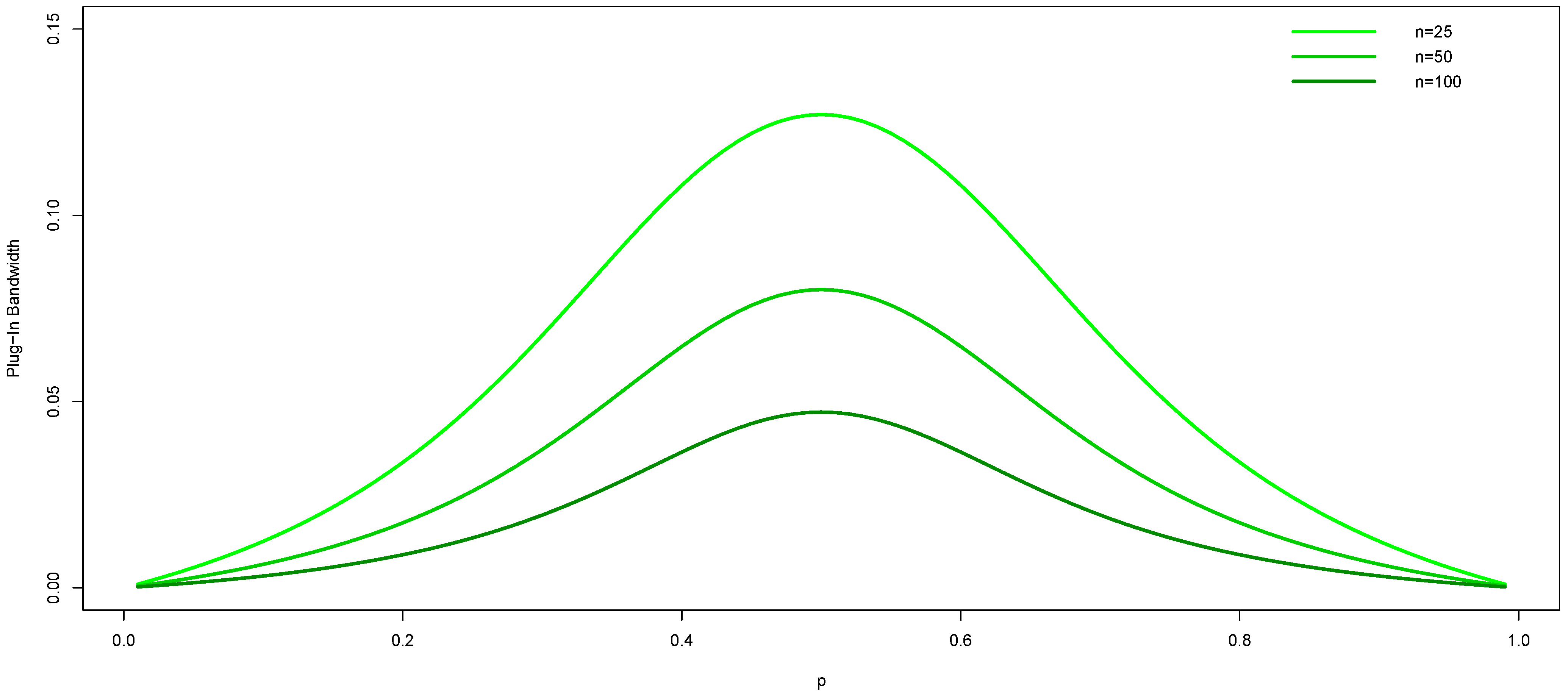
Figure 1 shows the plug-in bandwidths for three separate sample sizes (
, 50, and 100). We see that they are largest when the true probability is near uniform and they decrease as the sample size increases.
Figure 1.
Plug-in bandwidth for the Wang and van Ryzin kernel with two cells () for three different sample sizes ( and 100).
Figure 1.
Plug-in bandwidth for the Wang and van Ryzin kernel with two cells () for three different sample sizes ( and 100).
2.2.2. Three Categories ()
Similar to
Section 2.2.1,
is a root from the quintic equation
where the coefficients
E,
F,
G,
H,
I, and
J consist of parameters
n and
.
4 Although there exist no formula for roots, numerical methods can be deployed to solve for the roots of the higher order polynomial. Using Brent’s [
15] method, our algorithm finds the same outcome in essentially each setting (one unique real root and two pairs of imaginary roots).
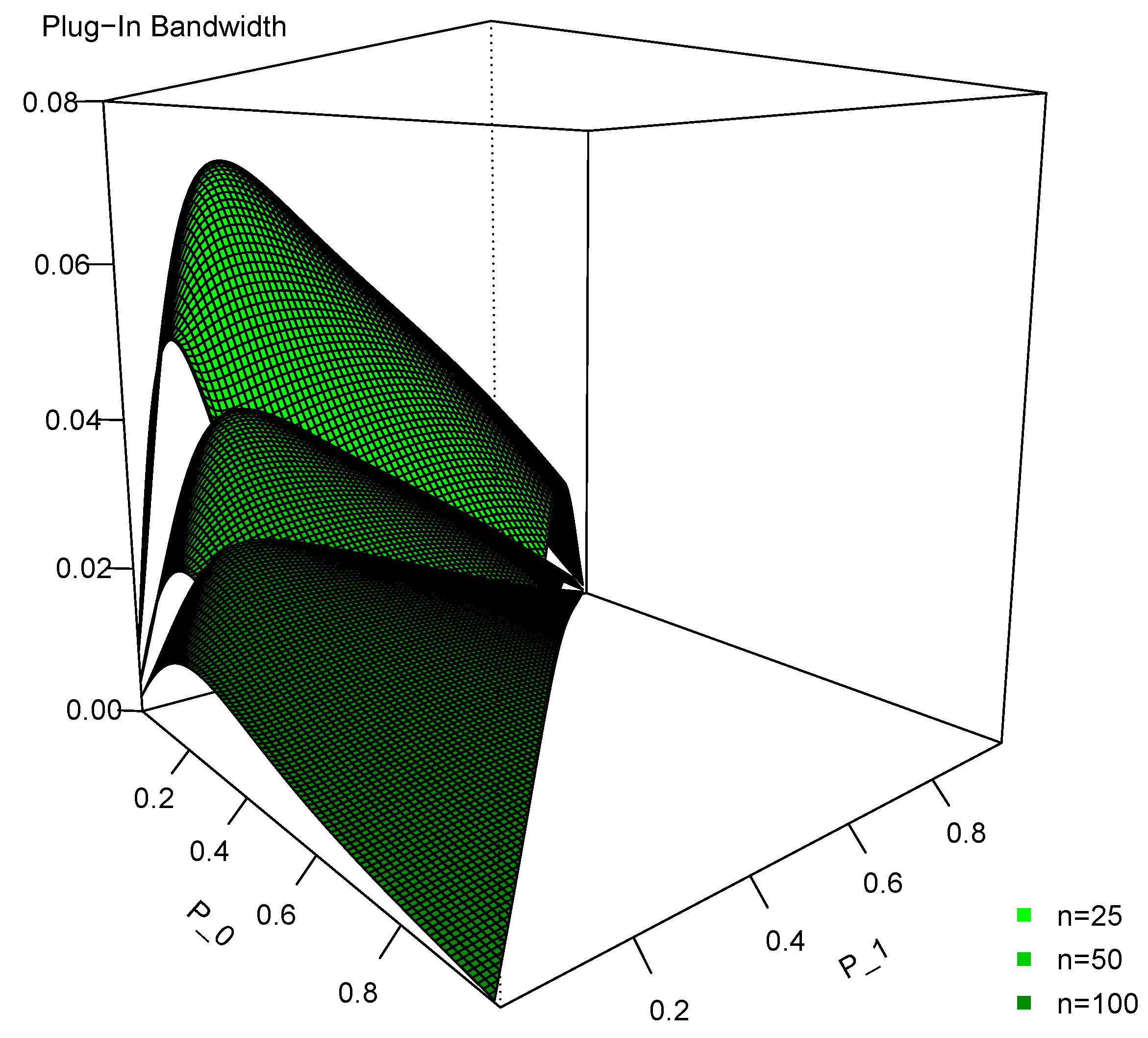
Figure 2 shows the plug-in bandwidths for three separate sample sizes (
, 50, and 100). We see that they are again largest when the true probability is near uniform and they decrease as the sample size increases.
Figure 2.
Plug-in bandwidth for the Wang and van Ryzin kernel with three cells () for three different sample sizes ( and 100).
Figure 2.
Plug-in bandwidth for the Wang and van Ryzin kernel with three cells () for three different sample sizes ( and 100).
2.2.3. Geometric Property of the Kernel Function
Notice from
Figure 1 and especially
Figure 2 that the plug-in bandwidths are relative small. Rajagopalan and Lall [
16] mention that weights for the Wang and van Ryzin kernel drop off rapidly because of the geometric form of the kernel function. They argue that this kernel should not be used to smooth sparse data and propose an alternative approach.
To circumvent the drop-off problem, Rajagopalan and Lall [
16] develop a discrete-version MSE optimal kernel which can be expressed in terms of the bandwidth and hence it is feasible to obtain the optimal bandwidth via minimizing MSSE. To avoid this problem with the Aitchinson and Aitken kernel, Titterington [
7] derives an optimal bandwidth with the restriction that it must be greater than or equal to one-half.
2.3. (Unordered) Li and Racine
Li and Racine [
11,
12] and Ouyang, Li, and Racine [
4] develop unordered and ordered kernel functions which are similar to Aitchison and Aitken’s [
6] and Wang and van Ryzin’s [
10] kernel functions, respectively. The former is introduced here and the latter will be shown in the next subsection. Their unordered kernel function is
where
. This kernel has a similar limiting behavior to the Aitchison and Aitken kernel: when
,
collapses to the indicator function
and when
,
gives uniform weighting.
The plug-in bandwidth (
) for this kernel function is
converges to 0 (the lower bound) as
n goes to infinity, but doesn’t converge to a specific value as
approximates the uniform distribution because
c does not enter the kernel function directly.
For the specific cases where
and 3,
is given as
and
respectively.
2.4. (Ordered) Li and Racine
The ordered Li and Racine kernel function is defined as
where
and
has the same intuition as for the Wang and van Ryzin kernel (and has the same limiting behavior as the Li and Racine unordered kernel function).
For the case where
,
can be derived as
and can be shown to be identical to Equation (
3) and this is intuitive given that we have two categories.
For the case where
,
is a root from the cubic equation
where the coefficients
K,
L,
M, and
N consist of
n and
.
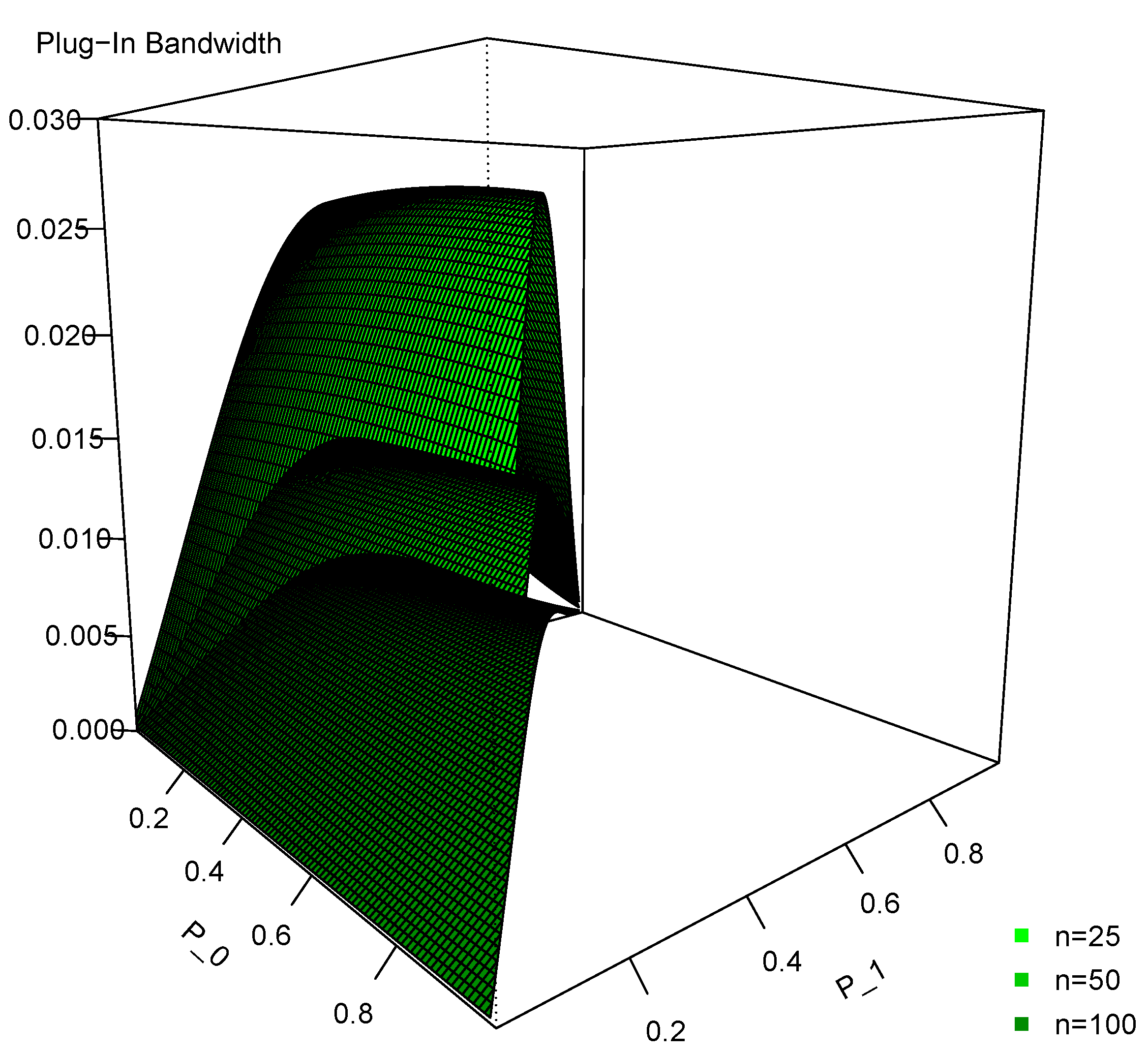
5Figure 3 shows the plug-in bandwidths for three separate sample sizes (
, 50, and 100). We again see that they decrease as the sample size increases. However, the curves are relatively flat. Specifically, for any given
and
n,
L and
N are fixed, because a trade-off occurs between
and
in
K and
M. In other words,
K and
M are essentially constant when
(or
) changes. Therefore, the impact in the plug-in bandwidth of a change in
(or
) is limited. Again, the figure shows that the plug-in bandwidth is relatively small in each case and the logic is the same as we discussed for the Wang and van Ryzin kernel.
Figure 3.
Plug-in bandwidth for the Li and Racine ordered kernel with three cells () for three different sample sizes ( and 100).
Figure 3.
Plug-in bandwidth for the Li and Racine ordered kernel with three cells () for three different sample sizes ( and 100).
2.5. Plug-in versus Cross-Validated Bandwidths
To evaluate the performance of the plug-in bandwidth, we compare the plug-in bandwidth with a data-driven method, such as least-squares cross-validation (LSCV).
6 The feasible cross-validation function proposed by Ouyang, Li, and Racine [
4] is given as
where
is the leave-one-out estimator of
. If we were to use the Aitchison and Aitken kernel, the kernel estimator of
can be written as
Similarly, the leave-one-out estimator of
can be written as
Taking the first derivative of the cross-validation function with respect to λ and setting this equal to zero leads to the optimal bandwidth
where
. Note that this is a closed form solution and hence we could perform cross-validation without an optimization function.
For comparison, if we expand Equation (
2), it can be rearranged such that
We can see that Equations (
4) and (
5) are asymptotically equivalent.
7 However, they are different in finite samples. The impact of this will be discussed further in the next section. It is straightforward to derive the cross-validated bandwidth for the unordered Li and Racine kernel, but simple closed-form comparisons for the ordered kernels (we believe) do not exist. That being said, the cross-validated bandwidth for the ordered kernels are similar to what we show in
Section 2.2 and
Section 2.4. For example, for the Wang and van Ryzin kernel with
, both the plug-in and cross-validated bandwidths are a unique real root from a quintic equation.
3. Simulations
3.1. Settings
For our simulations, the data are generated (as shown in
Table 1 and
Table 2) by using multinomial (
and 3) and beta-binomial (
) distributions for unordered and ordered kernels, respectively (we consider four scenarios for each distribution). The beta-binomial distribution is the discrete-version the beta distribution and has two parameters (α and β) that can determine the first four moments (see [
17,
18] for details on its simulation). We use the value
as a measure of the design. We have a uniform design as
r goes to one and empty cells (few observations in almost all categories) as
r goes to infinity. We consider two measures (relative bias and relative MSE) to evaluate the performance of the plug-in bandwidth and take the average over
replications for each sample size
, 50, and 100. The measures considered are as follows:
- (1)
Ratio of bias of the estimated probability function with the cross-validated bandwidth to that with the estimated plug-in bandwidth,
- (2)
Ratio of mean square error of the estimated probability function with the cross-validated bandwidth to that with the estimated plug-in bandwidth,
Table 1.
Monte Carlo simulation scenarios for unordered kernels.
Table 1.
Monte Carlo simulation scenarios for unordered kernels.
| Scenario | c = 2 | c = 3 |
|---|
| Probability | r | Probability | r |
|---|
| i | p0 = 0.25, p1 = 0.75 | 3.0 | p0 = 0.15, p1 = 0.35, p1 = 0.50 | 3.3 |
| ii | p0 = 0.30, p1 = 0.70 | 2.3 | p0 = 0.25, p1 = 0.30, p1 = 0.45 | 2.5 |
| iii | p0 = 0.40, p1 = 0.60 | 1.5 | p0 = 0.25, p1 = 0.35, p1 = 0.40 | 1.6 |
| iv | p0 = 0.50, p1 = 0.50 | 1.0 | p0 = 1/3, p1 = 1/3, p1 = 1/3 | 1.0 |
Table 2.
Monte Carlo simulation scenarios for ordered kernels.
Table 2.
Monte Carlo simulation scenarios for ordered kernels.
| Scenario | c = 3 |
|---|
| Probability | Shape Parameters | r |
|---|
| i | p0 = 0.50, p1 = 0.33, p2 = 0.17 | α = 1, β = 2 | 2.9 |
| ii | p0 = 0.25, p1 = 0.50, p2 = 0.25 | α = 50, β = 50 | 2.0 |
| iii | p0 = 0.40, p1 = 0.20, p2 = 0.40 | α = 0.33, β = 0.33 | 2.0 |
| iv | p0 = 1/3, p1 = 1/3, p2 = 1/3 | α = 1, β = 1 | 1.0 |
4. Empirical Illustrations
In this section we consider two empirical examples to complement our Monte Carlo simulations. While each of these examples is simplistic, they will shed insight into the difference between estimated bandwidths when applied to empirical data. Specifically, we hope to see the relative sizes of the bandwidths from each procedure as well as examine how they change with the sample size.
For unordered kernels, we consider the travel mode choice (between Sydney and Melbourne, Australia) data from [
20]. This data consists of
observations and
categories (air, train, bus, and car). We note here that we likely have a non-uniform design as the relative proportions for air, train, bus, and car are 0.28, 0.30, 0.14, and 0.28, respectively. For ordered kernels, we consider the well-studied salary data from [
21]. This data consists of
observations. Instead of the
or 28 cell cases typically considered, we further condense the number of cells to
to make closer comparisons to our simulations. We also appear to have a non-uniform design here as the relative proportions for low, middle, and high salaries are 0.26, 0.49, and 0.25, respectively. For each data set, we consider both the full-sample size as well as random sub-samples of size
, 50 and 100 (again, consistent with the simulations).
Table 5 gives the plug-in and cross-validated bandwidths for each kernel for each data set for each sample size. The most glaring observation is that the plug-in bandwidth is always smaller than the corresponding cross-validated bandwidth, sometimes strikingly so. Further, the relative difference is not uniform across ordered and unordered kernels. We see that the plug-in and cross-validated bandwidths are most similar for the Aitchinson and Aitken kernel. The ratio of the cross-validated to the plug-in bandwidth is just above unity. However, for each of the other kernels, this ratio is many times larger (and increases with the sample size). Finally, as expected, the bandwidths each tend towards zero (non-uniform design) as the sample size increases.
Table 5.
Empirical comparisons between plug-in and cross-validated bandwidths.
Table 5.
Empirical comparisons between plug-in and cross-validated bandwidths.
| n | Travel Mode (c = 4 ) | Salary (c = 3 ) |
|---|
| λAA | λULR | λWR | λOLR |
|---|
| PI | LSCV | PI | LSCV | PI | LSCV | PI | LSCV |
|---|
| 25 | 0.2138 | 0.3114 | 0.0117 | 0.1507 | 0.0440 | 0.2324 | 0.0267 | 0.1625 |
| 50 | 0.1950 | 0.2688 | 0.0062 | 0.1226 | 0.0224 | 0.1495 | 0.0137 | 0.0930 |
| 100 | 0.1719 | 0.2253 | 0.0032 | 0.0969 | 0.0123 | 0.0811 | 0.0067 | 0.0475 |
| Full | 0.1372 | 0.1687 | 0.0015 | 0.0676 | 0.0083 | 0.0565 | 0.0046 | 0.0316 |
5. Conclusions
Bandwidth selection is sine qua non for practical kernel smoothing. In the continuous data setting, aside from being well-studied, plug-in methods are praised for their performance relative to data-driven methods. Yet, migrating to the discrete setting, relatively little discussion on plug-in bandwidth selection exists, especially in comparison to the matured literature surrounding the continuous data setting. Here, we offer a simple plug-in bandwidth selection rule for univariate density estimation where the data possesses a multinomial distribution and compare with the corresponding data-driven bandwidth selectors.
Simulation results show that plug-in bandwidths for unordered kernels perform well in a non-uniform design; similar to their performance in continuous data settings. We see that the plug-in bandwidths for ordered kernels are relatively small and provide little smoothing. Moreover, at least in the case of three categories, the plug-in bandwidth for the Li and Racine ordered kernel possesses a flatness property. The empirical examples show that the plug-in bandwidths are smaller than the cross-validated bandwidths, quite different than the continuous data setting where it is commonly seen that plug-in bandwidths tend to provide more smoothing than data-driven bandwidths.


