Article

Modeling Autoregressive Processes with Moving-Quantiles-Implied Nonlinearity

1
Faculty of Economics, Konan University, 8-9-1 Okamoto, Higashinada-Ku, Kobe 658-8501, Japan
2
Department of Econometric Analysis, Faculty of Mathematics and Informatics, Vilnius University, Naugarduko 24, Vilnius LT-03225, Lithuania
*
Author to whom correspondence should be addressed.
Econometrics 2015, 3(1), 2-54; https://doi.org/10.3390/econometrics3010002
Submission received: 31 July 2014 / Accepted: 19 December 2014 / Published: 16 January 2015
(This article belongs to the Special Issue Non-Linear Regression Modeling)

Abstract

:
We introduce and investigate some properties of a class of nonlinear time series models based on the moving sample quantiles in the autoregressive data generating process. We derive a test fit to detect this type of nonlinearity. Using the daily realized volatility data of Standard & Poor’s 500 (S&P 500) and several other indices, we obtained good performance using these models in an out-of-sample forecasting exercise compared with the forecasts obtained based on the usual linear heterogeneous autoregressive and other models of realized volatility.
JEL classifications:
C22; C58

1. Introduction

In this study, we propose a nonlinear autoregressive time series model where the nonlinearity stems from the presence of moving order statistics-linked quantities in the data generating process (DGP). Moving order statistics and their linear filters (L-statistics) have a long history, and they have been used extensively in statistics and engineering studies to improve the precision of models, for change detection, robust inference, characterization of distributions, etc. (see [1,2,3,4,5,6], and many others). However, to our knowledge, there is no time series model proposed that includes and models the effects of moving order statistics (or moving sample quantiles as their generalization). Hence, the main purpose of this paper is to introduce such a non-linear autoregressive model where non-linearity is caused by the presence of moving sample quantiles.
In econometrics and time series analysis, the implied nonlinearity of moving order statistics appears to have escaped the attention of researchers at theoretical and empirical levels. However, the exceptions are models of extremes (see [7,8,9] and, e.g., [10,11], for more recent overviews of modeling max-stable processes and time series extremes). Other than in these models, we consider the whole range of moving order statistics to characterize the influence of moving order statistics-linked quantities on the response itself in an additive model.
Considering a range of order statistics in moving samples allows us to capture the effects related to the influence of different ordered sizes of the realizations present within a considered window and the effects of a local empirical distribution of recent values for a modeled process 1.
The importance of events of different magnitude is well recognized in finance and econometrics research, e.g., sizeable shocks in financial markets can generate very different behaviors of market participants due to differences in the intensity of interactions in the real and financial sectors (see, e.g., [14,15]). Thus, various regime switching, threshold autoregression and smooth transition models have been used extensively to capture and gauge these effects (see, e.g., [16,17,18,19,20,21] for overviews of such models). In the models with moving order statistics and moving sample quantiles (MQ) as their generalization, the order statistics-linked effects directly reveal the importance of the different sizes of realizations observed within a sample. However, these models do not contain any exogenously given threshold levels, because they evolve endogenously depending on the realizations of the recent values of the process. Furthermore, they convey an infinite number of potential regimes, which are represented by the specific local distributions that are characterized by the order statistics/quantiles in the moving samples.
There are many possible causes for time-varying distributions. For instance, in line with the behavioral finance paradigm (see, e.g., [22,23]) it is shown that the (stationary and invariant) probability distribution of returns varies substantially with the changing structure of the market, e.g., the fractions of boundedly rational traders and trend followers, the speed of their adjustments, etc. In regular periods of time, the segmentation and strategies of investors can be insufficiently discriminatory, because of market-neutral investing, order-splitting strategies and/or sufficient liquidity present in the market. However, whenever certain exposures to systemic risk substantially affect the general expectations and supply/demand structure, the nature of market participants who rely more or less heavily on market-neutral investing strategies versus those who depend more on momentum-based strategies, or particular style of investing, can become important. Thus, the local distribution might become informative in terms of the pressures that exist in the market during the particular historical period under consideration.
In finite samples, a meaningful estimate of the unconstrained effects of all the moving order statistics might become cumbersome whenever the length of a relevant moving window (sub-sample) is relatively large. Therefore, we extend the analysis to models with moving sample quantiles as the natural aggregates of moving order statistics. In general, models with moving order statistics/quantiles can be represented as a model with random coefficients (see, e.g., [24] for the latter). However, the random coefficients are highly dependent in these models due to the overlapping moving samples. The usage of moving order statistics/quantiles imposes a certain structure, and it has some specificity; however, it also requires some additional theoretical underpinning. Thus, before turning to the empirical part, which aims at illustrating the application of the model, we introduce a minimal set of tools that are needed to evaluate the statistical properties of processes with moving quantiles, define some properties of a simple estimator of parameters and propose a statistical test for evaluating the significance of MQ terms.
We illustrate the value of using MQs for modeling and forecasting the empirical realized volatility series (see, e.g., the overviews by [25,26] or [27]). First, we show that coupling the MQs with the constrained linear autoregression, where we use the exponential Almon polynomial restriction that is employed extensively in realized volatility forecasting models based on the mixed frequency data sampling (MIDAS) literature (see, e.g., [28,29]), robustly outperforms the standard benchmark, i.e., the heterogeneous autoregression model of realized volatility (HAR-RV) proposed by [30], as well as other constrained and unconstrained models that do not contain the MQ terms. Second, as hypothesized above, we observe that the precision and forecasting ability of MQ terms is better during a more volatile period.
The remainder of this paper is structured as follows. The model is introduced in Section 2. In Section 3, we analyze some statistical properties of the model, as well as its estimation and testing. Section 4 evaluates the empirical relevance of MQs for modeling and forecasting the realized volatility. The robustness analysis and some extensions of the empirical modeling are contained in Section 5. The proofs of the propositions are given in Appendix A (unless explicitly stated otherwise), while Appendix B to Appendix E provide additional information about some properties of the process and the empirical applications.

2. Model with MQs and Its Functional-Coefficient Form

Consider a discrete regularly-spaced, real-valued time series sequence { x t } t = 1 T , T N and a positive integer k < T . For t k , let x k , t : = ( x t , x t - 1 , , x t - k + 1 ) be the respective subsample of the sequence. Then, for each time period, the corresponding sample quantile vector is denoted by:
q m , t : = ( q t ( 1 ) , q t ( 2 ) , , q t ( m ) ) = q ( x k , t ) q t ( i ) : = q α i , t , i = 1 , 2 , , m k
where q : R k R m represents a measurable function that maps k observations into the m-dimensional vector of the sample quantiles that correspond to predefined α i [ 0 , 1 ] , i = 1 , 2 , , m . It is clear that q m , t is a function (also) of k, but for presentational simplicity, we omit this index and assume that k is pre-fixed. It is usually convenient to impose m < k , since this not only yields a smaller number of parameters for later estimation, but it also avoids some problems of identification, which are illustrated at the end of this section.
The model under consideration is as follows:
x t = c + ϕ x k , t - 1 + θ q m , t - 1 + ξ t
where c, ϕ and θ are a constant and the two additional real-valued parameter vectors of the respective dimensions, respectively, and ξ t denotes the zero mean i.i.d. error term, which has an absolutely continuous distribution function with positive density almost everywhere. It should be noted that in order to avoid additional heavy indexing, we assume without loss of generality that the order of linear autoregressive components and the window length used to calculate the sample MQ terms is the same, i.e., it is equal to k. In the sequel, the model under consideration is abbreviated as AR (autoregressive)-MQ where appropriate.
The sample quantiles are weighted averages of consecutive order statistics with several alternatives used in defining the weights (see, e.g., [31]). In order to facilitate our proofs and to allow for various alternatives of sample quantiles, in the following, we introduce a representation of sample quantiles based on an indicator function abstracting from the specific weighting problem:
1 I i , j , t : = 1 I q t - 1 ( i ) 0 and x t - j = min x { x t - r , r = 1 , 2 , , k } : x q t - 1 ( i ) + 1 I q t - 1 ( i ) < 0 and x t - j = max x { x t - r , r = 1 , 2 , , k } : x q t - 1 ( i )
and:
δ i , j , t : = δ i ( x t - j ) = max δ ( 0 , 1 ] δ 1 I q t - 1 ( i ) = δ x t - j
where i { 1 , 2 , , m } , j { 1 , 2 , , k } and t k . For instance, if the p-th ordered value of a sequence is used to represent the respective α p k quantile, then there would exist some j { 1 , 2 , , k } , such that δ i , j , t = 1 and 1 I i , j , t = 1 I x t - j = q t - 1 ( i ) for every i = 1 , 2 , , m .
Given these definitions, let us expand the term θ q m , t - 1 of model in Equation (1), for the clarity of exposition, as follows
θ q m , t - 1 = i = 1 m θ i q t - 1 ( i ) = i = 1 m θ i j = 1 k 1 I i , j , t δ i , j , t x t - j = j = 1 k i = 1 m θ i 1 I i , j , t δ i , j , t x t - j = j = 1 k θ j , t x t - j , where θ j , t : = i = 1 m θ i 1 I i , j , t δ i , j , t , j = 1 , 2 , , k
Since δ i , j , t [ 0 , 1 ] holds for any appropriate triplet ( i , j , t ) , it is clear that the time-varying parameters θ j , t are bounded by | θ j , t | i = 1 m | θ i | , j = 1 , 2 , , k , t Z .
Then, by denoting θ ˜ ( x k , t - 1 ) : = ( θ 1 , t , θ 2 , t , , θ k , t ) , we can write model, given by Equation (1), as:
x t = c + β t x k , t - 1 + ξ t β t = ϕ + θ ˜ ( x k , t - 1 )
In this case, β t is bounded provided that ϕ and θ are bounded. In the general case, it is also clear that the time-varying coefficients are non i.i.d. This representation takes the form of the functional-coefficient autoregressive models of [24]. However, the direct usage of the analytical results provided therein leads to a less explicit characterization of the statistical properties of the specific model under consideration (see Remark 2 in the next section).
Next, we use the example provided below to illustrate that we must be careful whenever m = k is applied, because model in Equation (3) might become unidentified, since the quantile part itself encompasses a (restricted) linear combination of original variables. For simplicity of presentation, we impose c = 0 and consider the case where m = k = 2 with maximum and minimum in q 2 , t = ( q α 1 , t , q α 2 , t ) , i.e., with α 1 = 1 and α 2 = 0 . For this simple example, we can set δ i , j , t = 1 for all t and i , j { 1 , 2 } without loss of generality. Let a t : = 1 I 1 , 1 , t . Note that in the case under consideration, 1 I 2 , 1 , t = 1 I 1 , 2 , t = 1 - a t , while 1 I 2 , 2 , t = a t . Then, putting Equation (2) in Equation (3) gives:
x t = ϕ 1 + θ 1 1 I 1 , 1 , t + θ 2 1 I 2 , 1 , t x t - 1 + ϕ 2 + θ 1 1 I 1 , 2 , t + θ 2 1 I 2 , 2 , t x t - 2 + ξ t = ϕ 1 + θ 1 a t + θ 2 ( 1 - a t ) x t - 1 + ϕ 2 + θ 1 ( 1 - a t ) + θ 2 a t x t - 2 + ξ t = ϕ 1 + θ 2 + ( θ 1 - θ 2 ) a t x t - 1 + ϕ 2 + θ 1 + ( θ 2 - θ 1 ) a t x t - 2 + ξ t
with the non-identified set of parameters due to a missing additional restriction.
The result of this simple example extends to the general case of m = k , whenever the sample quantile definition leads to it, for all t = 1 , 2 , , T and i = 1 , 2 , , m , x { x t - j } j = 1 k , such that 1 I x = q t - 1 ( i ) = 1 ; for instance, whenever size-ordered sub-sequences are used directly, as in the ordered weighted aggregation approach (see, e.g., [32]).

3. Some Characterizations of the MQ Process

3.1. Stationarity and Existence of Moments

Given the above representation, it is easy to establish some properties of the process using the standard results. In Proposition 1, the existence of a strictly stationary solution is obtained based on Theorems 2.2 and 2.4 in [33], particularly based on the geometric ergodicity Theorem 1 with Corollary 1 of [34] with respect to the geometric ergodicity of model-related Markov chain. The results of [24,35] could also be invoked, as noted in Remark 2. If not stated otherwise explicitly, the proofs are presented in Appendix A.
To proceed, let us also introduce, for some real-valued vector z = ( z 1 , z 2 , , z n ) , a norm z 1 : = i = 1 n | z i | , and for a real-valued matrix A, the - norm A : = max i j | A i , j | .
Proposition 1. 
Suppose that model in Equation (1) holds for all t Z with an additional requirement that the error term ξ t satisfies E | ξ t | < . Furthermore, assume that | | ϕ | | 1 + | | θ | | 1 < 1 . Then, there exists a stationary distribution of the related Markov chain, such that { x t , t = 1 , 2 , } defined by Equation (1) and initiated from the stationary distribution is strictly stationary.
Remark 1. 
The strict stationarity and ergodicity of { x t } implies that the elements of { β t } and { q m , t } are also strictly stationary and ergodic (see, e.g., Theorem 3.5.8. in [36] or Theorem 6.1.1. in [37]).
Remark 2. 
Alternatively, to derive the geometric ergodicity, we could rely directly on [35] and, similar to [38], use a sufficient condition that the joint spectral radius of the companion form of the model is less than one. Furthermore, the [24] requirement could be employed for the roots of the characteristic polynomial λ k - c 1 λ k - 1 - - c k = 0 , where c j : = s u p x R k | ϕ j + θ j , t | , j = 1 , 2 , , k , need to be inside the unit circle, which was shown by [39] to be a sufficient condition for the aforementioned joint spectral radius condition to hold. However, it is numerically demanding to check the joint spectral radius condition for larger values of k, whereas the [24] condition becomes less explicit without further specification of the quantile structure.
In the following analysis, we rely on the condition stated in Proposition 1. In this case, the question of the existence of the moments of the process can be answered in a straightforward manner using Theorem 2 from [40].
Proposition 2. 
Suppose that model in Equation (1) holds for all t Z and that E | ξ t | r < for some r 1 . Then, E | x t | r < .

3.2. Estimation

Now, we turn to the issue of the estimation of the parameters of the model using the ordinary least squares (OLS) estimator. Suppose that we have observations { x t } t = 1 T , T N . Let z t : = 1 , x k , t - 1 , q m , t - 1 . Note that for an identified model in Equation (1), 1 T - k t = k + 1 T z t z t is positive definite almost surely (a.s.); thus let us consider the OLS estimator:
η ^ = t = k + 1 T z t z t - 1 t = k + 1 T z t x t
Proposition 3. 
Assume that model in Equation (1) is identified with positive integers m < k and that it holds for all t Z with E ξ t 2 < . Furthermore, suppose that the conditions of Proposition 1 are satisfied. Then, η ^ η as T a.s. Furthermore, σ ξ - 1 t = k + 1 T z t z t 1 2 η ^ - η a N 0 k + m + 1 , I k + m + 1 .

3.3. Test for the MQ Terms

Next, we provide a test that is suitable for evaluating the following set of hypotheses:
H 0 : θ = 0 m
H 1 : θ 0 m
i.e., the null hypothesis is that the MQ effects are absent from model in Equation (1). In order to characterize the test, let us define some further notations:
x ˜ k , t : = ( 1 , x k , t ) , t = k + 1 , k + 2 , , T X : = ( x ˜ k , k + 1 , x ˜ k , k + 2 , , x ˜ k , T ) Q : = ( q m , k + 1 , q m , k + 2 , , q m , T ) φ : = ( c , ϕ )
Then, we can write the unrestricted and restricted versions of Equation (1), respectively, as:
x = X φ + Q θ + ξ
x = X φ + u , u : = Q θ + ξ
In addition, let us introduce:
(1) the OLS estimator-linked residuals of the restricted Equation (9) in an auxiliary regression form:
u ^ = M x = H θ + v
where M : = I T k - X X X - 1 X , H : = M Q , and v : = M ξ ;
(2) and the OLS estimator of θ in Equation (10), which is defined by:
θ ^ = H H - 1 H u ^
Then, the following result can be employed to test the hypotheses stated above.
Theorem 1. 
Suppose that model in Equation (1) holds where the conditions in Proposition 3 are satisfied and that for some positive constant σ ξ 2 , ξ t i . i . d . ( 0 , σ ξ 2 ) for all t Z . Then, under H 0 : θ = 0 m , it holds that:
θ ^ H H θ ^ / σ ξ 2 a χ 2 ( m ) ,
whereas the statistic diverges with a probability of one under θ 0 m .
In model, given by Equation (1), and the test presented above, the linear autoregressive parameters are supposed to be unconstrained. In some situations, the linear autoregression coefficients might be constrained to satisfy some low-dimensional parametric functional restriction, i.e.,
ϕ i = f ( ψ , i ) , ψ R q , q < k , i = 1 , 2 , , k
This constraint reduces the number of parameters that need to be estimated by k - q > 0 . Correspondingly, because the number of degrees of freedom is higher, the size and power of the test for the presence of MQs could be enhanced. In order to characterize a test whenever model in Equation (1) satisfies this restriction, let us also define:
f ( ψ ) : = ( f ( ψ , 1 ) , f ( ψ , 2 ) , , f ( ψ , k ) ) D : = f ( ψ ) / ψ M r : = I T k - X D D X X D - 1 D X H r : = M r Q u ^ r , t : = M r x = H r θ + v r , v r = M r ξ θ ^ r : = H r H r - 1 H r u ^ r , t
where u ^ r , t denotes a residual term of model in Equation (9), which is estimated with the nonlinear least squares while considering the restriction defined by Equation (12), whereas θ ^ r represents the OLS estimator of θ in the corresponding auxiliary regression of u ^ r , t on H r . Now, we can state the following auxiliary result.
Remark 3. 
Suppose that in addition to the conditions of Theorem 1, the linear autoregressive coefficients in model Equation (1) satisfy constraint given by Equation (12) and f ( · ) is twice differentiable with respect to the hyper-parameter vector ψ . Then, under H 0 : θ = 0 m , it holds that:
θ ^ r H r H r θ ^ r / σ ξ 2 a χ 2 ( m )
whereas the statistic diverges with a probability of one under H 0 : θ 0 m .

3.4. Finite Sample Properties of the Parameter Estimator

In this subsection, we use simulations to investigate the small-sample properties of the OLS estimator of parameters, as defined in Equation (5), in models having MQ terms. Namely, relying on 2,000 simulations (at each node splitting the interval [0,500] into 10 equal parts) with the standard Gaussian error and 500 observations dropped at the initiation stage of the process, we report the bias and the mean squared error (MSE) of the estimator of parameters of both the linear autoregressive terms and the moving quantile. For the simplicity of comparison of the results of the purely linear autoregression with the AR-MQ, we concentrate on the case where only the first order linear autoregression term and a single moving sample quantile (either moving median or moving maximum) are present in model, given by Equation (1), allowing for various window lengths of the MQ term (the considered window sizes k { 5 , 20 , 60 } in connection with the empirical application presented in Section 4). For comparability, we set both values of parameters (of the linear autoregression and the MQ term) to 0.4, which satisfies the requirement stated in Proposition 1. For informativeness, we also report separately the bias and the MSE of a purely linear autoregression and a model with only the MQ term by setting the parameter of the remaining term to zero in the AR-MQ model.
Figure 1 plots the bias (the upper row of figures) and the MSE (the lower row of figures) of the OLS estimator of AR-MQ parameters. Different colors identify different parameters under investigation: the results of estimation of the autoregressive parameter in a pure autoregression are depicted in red; the results of estimation of the MQ term in a pure MQ model are depicted in blue (the corresponding solid and dashed lines identify the moving maximum and moving median, respectively); the results of estimation of the autoregressive parameter and the MQ parameter in the AR-MQ model are depicted in black and green, correspondingly. For the MQ parameter, the solid and dashed lines again signify the moving maximum and moving median, respectively.
Figure 1. The bias and the mean squared error of the OLS estimator as in Equation (5) of parameters of the autoregressive moving sample quantiles (AR-MQ) model with the first-order linear autoregressive and the moving maximum or moving median term from the indicated window sizes. Colors identify different parameters under investigation: red, autoregressive parameter in a pure autoregression (AR in AR); blue, MQ term in a pure MQ model (MQ in MQ); black, autoregressive parameter in the AR-MQ model (AR in AR-MQ); green, MQ term in the AR-MQ model (MQ in AR-MQ). The solid and dashed lines (both blue and green) are used to identify the moving maximum and moving median, respectively.
Econometrics 03 00002 g001
Comparing the results obtained for the MQ terms with the ones for the linear autoregressive terms, it is obvious that, in order to get a satisfactory precision, one needs to have sample sizes much larger than the window of the MQ effects. It can be seen that the MSE of the estimator of the moving maximum parameter reduces to the MSE levels about twice as large as that of the estimator of the linear autoregressive term only for the sample sizes about twenty-times larger than the MQ window. Further, an even larger increase in the relative size of observations is required in order to achieve the same relative precision whenever the moving median is present.

3.5. Finite Sample Properties of the MQ Tests

In this subsection, we illustrate the behavior of the MQ tests using finite samples with 250, 500, 1,000 and 2,000 observations. We use Monte Carlo simulations with 2,000 iterations for each case. The parameterization of the DGP is motivated by the empirical application (see the last column of Table C1 in Appendix C, which shows some estimated empirical models of the realized volatility of returns in connection with the S&P 500 index), which is presented in the next section. The DGP is given by Equation (1) with k = 20 , ξ t n . i . d . ( 0 , 0 . 27 2 ) , the parameters of the linear part of the model satisfy the exponential Almon polynomial restriction, as given in Equation (15), with hyper-parameter values ψ 1 = 0 . 72 and ψ 2 = - 0 . 60 , and there is a single quantile effect parameter θ = 0 . 23 . This relies on the fact that in the empirical application with realized volatility data, only the moving median was sufficiently significant whenever the lags only up to one month were considered. However, in order to determine the different power properties of the tests in the presence of more central and more extreme quantiles in the DGP, we provide the simulation results for each quartile separately, i.e., where either only the minimum, or the first quartile, or the median, etc., is present in the data generating process. In the testing stage, all of the quartiles are used to estimate Equation (1) throughout all of the simulations. We use the quartiles as a certain grid with a manageable size of potentially relevant quantiles. The analogous results hold whenever other grids of quantiles are used instead of quartiles, such as quintiles, deciles, etc. It should be pointed out that by using a spectrum of quantiles instead of a particular one present in the DGP under the alternative, we lose some power of the test. However, it is highly unlikely that a particular true quantile will be known to a researcher in advance, and one of the general ideas of the proposed model is to evaluate whether there are some distributional effects captured by the (moving) quantiles. Hence, we prefer some loss of power to the case that could be much less relevant in practice.
We start with the empirical sizes of the tests using the unconstrained and constrained linear parts of the model, as formulated in Theorem 1 and Remark 3, respectively. Whenever the functional constraint on the parameters of the linear part of the model is considered, only two parameters ( ψ 1 and ψ 2 ) are estimated, instead of the 20 unconstrained linear autoregressive parameters in Equation (1). Figure 2 presents the simulation results under the null hypothesis stated in Equation (6), i.e., that the MQ terms are absent from the process. The red line corresponds to the unconstrained estimation (as in Theorem 1), whereas the blue line corresponds to the constrained estimation (as in Remark 3).
For the larger samples considered, the empirical sizes correspond well with the standard nominal size levels of the test (e.g., at 1%, 5% and 10% significance levels). In the case of T = 250 , the tests are undersized and would require some bootstrap-based inference. It can be seen that the constraint marginally improves the precision. In the other samples considered, the deviations from the nominal significance levels are small, if any, especially at the typical significance levels applied. Hence, in the following, we report the uncorrected power simulation results.
Figure 2. Distribution of the empirical sizes of the tests under H 0 : θ = 0 . The red line corresponds to the unconstrained estimation of Equation (1) (as in Theorem 1), whereas the blue line corresponds to the estimation with the constrained linear autoregressive part (as in Remark 3).
Econometrics 03 00002 g002
Figure 3 reports the power of the test as in Theorem 1, separately for different sample sizes ( T = 250 ; 500 ; 1 , 000 ; 2 , 000 ) and for the cases where a single MQ outside the quartiles is present in the DGP.
Although the power of the test increases with the sample size in all of the cases, it is less powerful for more central quantiles (closer to the median) but more powerful in the presence of more extreme quantiles. The power relative to the moving median is the smallest, whereas the same power behavior is observed for the symmetric deviations from the median, i.e., min and max, the first and third quartiles, etc. For the values of θ 0 . 5 , the power of the test would almost triple, but in the case under consideration (i.e., θ = 0 . 23 ), detecting the presence of non-extreme MQs requires large samples.
Figure 3. Distribution of the empirical sizes of the test (as in Theorem 1) under H 1 : θ 0 . Each of the four figures represents the results with different sample sizes, where the five lines correspond to the presence of different quartiles in the data generating process (DGP) (minimum, first quartile, median, third quartile and maximum).
Econometrics 03 00002 g003
Figure 4 shows the analogous simulation results, where the functional restriction on the parameters in the linear autoregressive part of the model is considered, as in Remark 3. It can be seen that reducing the number of parameters under estimation produced a substantial increase in the power of the test. This is what we also observe in the empirical application that follows.
Figure 4. Distribution of empirical sizes under H 1 : θ 0 for the test with the constrained linear autoregressive parameters (as in Remark 3). Each of the four figures represents the results with different sample sizes, where the five lines correspond to the presence of different quartiles in the DGP (minimum, first quartile, median, third quartile and maximum).
Econometrics 03 00002 g004

3.6. Simulation Evidence on the Power against Other Non-Linearities

The aim of this subsection, which again relies on Monte Carlo simulations, is three-fold. First, it is to show that the MQ test (we use hereafter the one that corresponds to Theorem 1) has good sizes whenever more general short and long memory linear processes generate the data. Second, we show that the MQ test has power against a number of other non-linearities, including some that generate pseudo long memory features, e.g., because of the presence of structural breaks. Third, we reveal a very useful property that potentially allows us to identify the presence of the MQ effects. Namely, simulations show that the RESET 2 tests [41] fail to detect the moving quantiles’ non-linearity, irrespective of the orders used for the testing. Since the RESET tests have power against many other non-linearities, the significance of the MQ test and insignificance of the RESET tests could hint at the presence of the MQs.
In the sequel, we generate 2,000 realizations for each of the DGPs characterized in Table 1 3. Block L contains various short and long memory linear stationary processes. Block N contains several non-linear processes taken from 4 [42,43]. We augment this set of models with an additional one in the spirit of [44], where the unconditional moment is driven by a bounded cyclical deterministic function. Many of the considered models are well known to be capable of generating pseudo long memory features, such as slowly decaying sample autocorrelation function (see, e.g., [43]).
Besides the DGPs used in simulations, Table 1 also presents the summary information about whether the MQ test and the RESET tests (of orders from two to four) have power against the indicated specifications (in the testing stage, we use the autoregressive order k = 12 for both types of tests). Our summarizing inference relies on the behavior of empirical sizes observed in samples of 250, 500, 1,000 and 2,000, which are plotted in Figure 5 below in this section (for the linear models) and Figure B2 and Figure B3 in Appendix B (for the non-linear specifications against which the MQ test has and does not have power, correspondingly).
As can be seen, the MQ test has power against some other non-linearities as well, but it is mostly weaker than that of the RESET tests. The exception, putting aside the MQ processes themselves, is a process with Markov switching GARCH regimes (MS-GARCH), where the power of the MQ test is substantially greater than that of the RESET tests. On the other hand, in the cases of the AR-MQ DGPs, neither of the RESET tests have any power. This combination of powerful MQ and powerless RESETs is a unique situation from all of the considered ones. There could of course be other non-linearities (that we are not aware of as of yet) leading to the same finding, but such a situation points to the MQs as a potential neglected non-linearity.
Finally, Figure 5 plots the distribution of empirical sizes of the MQ test under the considered DGPs in Block L. It reveals that the empirical sizes track very closely the nominal ones, especially at the significance levels that are usually used in practice. Similar results (unreported) hold for the RESET tests, apart from the AR(20) case. This happens because in the testing, we fixed k = 12 , and the RESET test, being a general specification test, rejects the hypothesis of zero conditional expectation of errors in the misspecified model.
The analogous figures of the distribution of empirical sizes of the MQ test for the non-linear models are presented in Appendix B. Figure B3 collects the non-linear DGPs, where the MQ test fails to have power, and Figure B2 gathers the considered non-linearities against which the MQ test has power.
Table 1. Summary of DGPs used in simulations and some main findings.
BlockCodeType of ModelDGPPower Observed in Simulations:
MQ TestRESET Tests (Any)MQ More Powerful?
LinearL1AR(1) x t = 0.8 x t - 1 + ε t .
L2AR(2) x t = 0.5 x t - 1 + 0.3 x t - 2 + ε t .
L3ARMA (1,1) x t = 0.8 x t - 1 + ε t - 0.5 ε t - 1 .
L4AR(12) x t = i = 1 12 ϕ i x t - i + ε t , ϕ i = 0.8 / 12 , i = 1 , 2 , , 12 .
L5AR(20) x t = i = 1 20 ϕ i x t - i + ε t , ϕ i = 0.8 / 20 , i = 1 , 2 , , 20 . +
L6FARIMA (0,d,0) Δ d x t = ε t , d = 0.2 .
L7FARIMA(0,d,0) Δ d x t = ε t , d = 0.4 .
L8FARIMA(1,d,1) Δ d x t = 0.8 Δ d x t - 1 + ε t - 0.5 ε t - 1 , d = 0.2 .
L9FARIMA(1,d,1) Δ d x t = 0.8 Δ d x t - 1 + ε t - 0.5 ε t - 1 , d = 0.4 .
Non-linearN1SETAR x t = 0.8 x t - 1 ( 1 I x t - 1 < 0 - 1 I x t - 1 > 0 ) + ε t . ++
N2ESTAR x t = 0.8 x t - 1 1 - 1.5 ( 1 - e - x t - 1 2 ) + ε t . ++
N3LSTAR x t = 0.8 x t - 1 1 - 1.5 / ( 1 + e - x t - 1 ) + ε t . ++
N4BL x t = 0.8 x t - 1 ( 1 + 0.375 ε t - 1 ) + ε t . ++
N5MQ(q 0.5 ) x t = 0.3 x t - 1 + 0.5 q 0 . 5 ( 12 ) + ε t . ++
N6MQ(q 0.75 ) x t = 0.3 x t - 1 + 0.5 q 0 . 75 ( 12 ) + ε t . ++
N7MQ(q 1 ) x t = 0.3 x t - 1 + 0.5 q 1 ( 12 ) + ε t . ++
N8MS -GARCH x t = l o g ( r t 2 ) , r t = h t ε t , h t = 1 + 3 s t + 0.4 r t - 1 2 + 0.3 h t - 1 . +++
N9MS-AR x t = 0.8 x t - 1 ( 2 S t - 1 ) + ε t . +
N10MS-mean x t = 2 s t - 1 + ε t . +
N11RLS -NS x t = μ t + 5 ε t , μ t = μ t - 1 + j t η t , j t i . i . d . B ( 1 , 0.00001 ) +
N12RLS-S x t = μ t + ε t , μ t = ( 1 - j t ) μ t - 1 + j t η t , j t i . i . d . B ( 1 , 0.003 ) +
N13Trend-power x t = f t + ε t , f t = 3 t - 0 . 1
N14Trend-cycles x t = c t + ε t , c t = 0.3 sin ( 3 π t / n ) + sin ( 6 π t / n ) , t { 1 , 2 , , n } , n = 2 , 000 .
Notes: ε t n . i . d . ( 0 , 1 ) and η t n . i . d . ( 0 , 1 ) are mutually independent, as well as independent of any other contemporaneous random variable on the right side of a DGP equation. S t { 0 , 1 } and s t { 0 , 1 } come from the Markov chains with transition probabilities matrices P S and P s , such that vec ( P S ) = ( 0.9 , 0.1 , 0.25 , 0.75 ) and vec ( P s ) = ( 0.999 , 0.001 , 0.001 , 0.999 ) .
Figure 5. Distribution of empirical sizes of the MQ test for the data generated from the stationary short and long memory linear processes (DGPs from the L block in Table 1).
Econometrics 03 00002 g005

3.7. Some Empirical Features of Realizations of the AR-MQ Process

In this subsection, we use the simulations to reveal that typical empirical realizations of the AR-MQ processes possess two interesting (and inter-related) features often observed in empirical data. First, a typical realization of the AR-MQ processes is featured by the presence of apparent “structural breaks”. The easiest way to understand the reason for this is to consider the extreme quantiles. Given some large shock (a realization of the error of the model), it tends to keep the levels of the series high (if, e.g., the moving maximum is present in the model and a positive shock has been realized) or low (if, e.g., the moving minimum is present and a negative shock has occurred) for the period of the window of the moving quantile. The moving median will usually lead to less prominent effects.
The second (and related) feature observed for a typical realization of the AR-MQ processes is the slowly decaying sample autocorrelation function. Other than in the genuine, fractionally-integrated processes, the possibility of a pseudo long memory behavior appearing due to the presence of structural breaks is well known (see, e.g., [45,46,47,48,49], among many others). The MQ model proposed in this paper, while being stationary and ergodic, can produce, due to the presence of pseudo structural breaks, series having flat sample autocorrelation functions (ACFs). Other than in the regime-switching models, there is no explicit regime switching mechanism here, but the apparent changes of regimes can be prescribed to a certain probabilistic structure of the model.
Figure 6 plots the paths and the ACFs of simulated realizations generated from the AR-MQ model that was used in Subsection 3.5 with a moving median term, as motivated by the empirical application (see the last column of Table C1 in Appendix C). The usage of more extreme quantiles in the DGP would further lead to more pronounced features under discussion. In order to reveal the contribution of the MQ term to the shape of the ACFs, we also present the ACFs for the pure linear autoregressive part of the model by imposing a zero restriction on the MQ term in the model (the same realization of errors is used for comparability). The resulting ACFs connected with the linear model are presented in a column of figures on the right side.
Figure 6. The realizations of the AR-MQ model (with the moving median from the indicated window sizes k), their sample autocorrelation functions (ACFs) (middle) and the ACFs of the linear autoregressive (AR) processes obtained by restricting the parameter of the MQ part to zero in the AR-MQ model (right).
Econometrics 03 00002 g006
The sample ACFs of realizations only from the autoregressive linear part barely change with the increasing order k due to the swiftly decreasing autoregressive parameters (as implied by the imposed exponential Almon polynomial parameterization). On the other hand, the ACFs of realizations from the full AR-MQ process are clearly featured by the presence of “long memory”. As is evident from the plotted paths of the simulated realizations, such an effect appears due to the presence of ‘structural breaks’ generated by the moving quantile part of the model.
It can be also pointed out that, given the Gaussian errors of the model, realizations from the AR-MQ model retain the Gaussianity (see Figure B1 in Appendix B). The two features provided above seem to be among the main features established in the literature on the logarithm of realized volatility empirical series (see, e.g., [50,51,52,53], among other). Hence, in the sequel, we use this indicator for the empirical illustration of the usage of the proposed model.

4. Empirical Application

We use financial data to illustrate the empirical relevance of MQs by testing their significance in Subsection 4.1 and by evaluating the in-sample and pseudo out-of-sample forecasting precision of the models with and without the MQs in Subection 4.2. Our main goal in this section is to discuss some aspects of the building of the MQ model and to reveal that the MQs might be relevant, e.g., in the out-of-sample forecasting.
The daily realized variance data of the period January 3, 2000, to May 22, 2012, was obtained from the Oxford-Man Institute of Quantitative Finance website 5 by taking the first series in this dataset (5-min realized variance of S&P 500 (live) index). It was transformed to the corresponding logarithm of the annualized realized volatility series 6 (see 
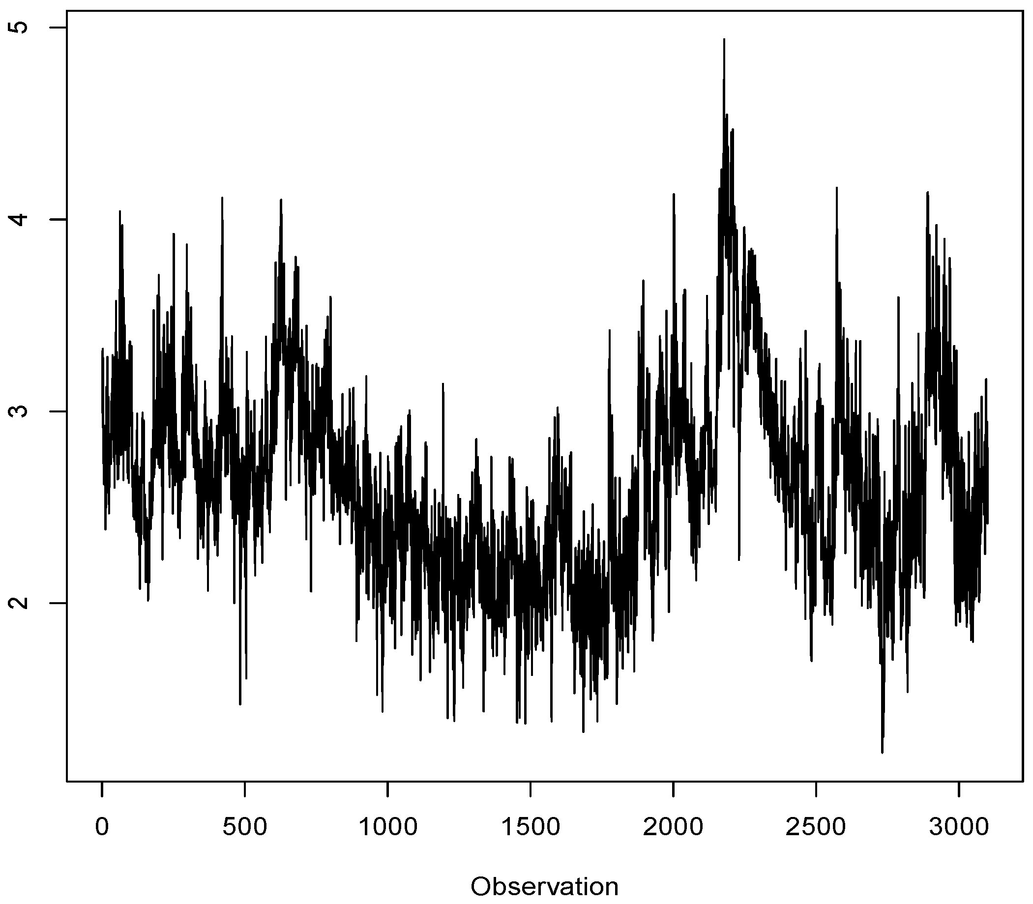
Figure 7). The effective sample size was about 3,000 observations. It can be seen that the middle third of the period is relatively less volatile compared with the other two-thirds of the observations, i.e., the periods with observations indexed by numbers 1–1,000 and 2,001–3,000. Hence, by looking at distinct periods, we can evaluate the behavior of the models in relatively calm and volatile periods.
Figure 7. Logarithm of the annualized realized volatility of the S&P 500 (live) index (5-min).
Econometrics 03 00002 g007
For each t Z , let a measure of the logarithm of annualized daily realized volatility be denoted by r v t . The linear forecasting equation of the one step ahead realized volatility based on its k past values is given by:
r v t = c + j = 1 k ϕ j r v t - j + ε t
where ε t represents an error term of a linear projection of r v t on its past values.
It is well known that certain restrictions on parameters { ϕ j } can enhance the forecasting precision of realized volatility series, where the two most representative examples are the HAR-RV model of [30] and the exponential Almon lag polynomial stemming from the restrictions used in the MIDAS regression models (see, e.g., [55]).
Although the HAR-RV model is most widely used as an approximation of the underlying RV process, [56] show, using a test proposed by [57], that, for the realized volatility of S&P 500 returns, the restriction on parameters implied by the HAR-RV model is empirically inadequate. On the other hand, the restriction implied by the exponential Almon polynomial constraint cannot be rejected (see ibidem). It should be pointed out that this constraint has already been used in modeling and forecasting the RV series also in the cases whenever there is only a single frequency, i.e., where single step ahead forecasts are produced, leaning on the autoregressive terms (see, e.g., [28,55,58]). The main aim here remains the same, i.e., to reduce the number of parameters and the connected variability of the estimators using a certain, quite flexible restriction. In the sequel, we employ both competing restrictions.
The restrictions on the parameters in the HAR-RV model take the following form:
ϕ j = ψ 1 + 1 5 ψ 2 + 1 k ψ 3 , for j = 1 1 5 ψ 2 + 1 k ψ 3 , for j = 2 , . . , 5 1 k ψ 3 , for j = 6 , . . . , k
where the coefficients ψ 1 , ψ 2 , and ψ 3 correspond to the daily, weekly and monthly effects, respectively. It should be noted that Equation (13) with restriction given by Equation (14) represents the average of the logarithmically transformed data. In most applications of the HAR-RV model with a logarithmic transformation, the logarithms of the averages over five and 21 days of realized volatility are employed rather than the averages of the logarithms. In our study, the former approach was dominated in both the in-sample and the out-of-sample precision analysis by the model given by Equation (13) with restriction as in Equation (14). In the following, we shorten the notation of the HAR-RV model to HAR.
The exponential Almon lag polynomial restriction applied in this study (this type of restriction is used widely, if not most usually, in MIDAS applications) has two real valued hyper-parameters, ψ 1 and ψ 2 , which are given by:
ϕ j = ψ 1 exp ψ 2 j s = 1 k exp ψ 2 s , j = 1 , , k
In the following, model in Equation (13) with the restriction given by Equation (15) imposed on the parameters is referred to as the ALMON model.
Analogous models that are augmented linearly with MQ terms produce the unrestricted and restricted versions of Equation (1). We start by testing the significance of MQ effects.

4.1. Significance of the MQ Terms

To test for the significance of the MQs, we need the (maximum) lag order k. In the case of the HAR model, we fix it at 20 lags. Although [59] found that the most informative maximum lag of aggregation could vary from 13 to 250 lags for different stocks, the normal maximum number of lags used in the HAR models is between 20 and 22, which correspond to the number of working days in a month. In our analysis, the difference between any of these three numbers was negligible. For example, the out-of-sample precision figures were unchanged when they were rounded to three digits (the precision level used to represent the relative out-of-sample forecast performance in Table 4). Furthermore, our analysis of an informative moving window, which is used to calculate the MQs, also signified 20 lags (as discussed later). Hence, to avoid an uninformative and heavy presentation of many, very similar models with virtually the same properties, we also fix the number of lags for the HAR model at 20 periods.
In addition, in unrestricted Equation (13) or the MIDAS-type models, the lag order is usually selected based on some information criteria. In our case, for both the unrestricted and the ALMON models, k = 12 is selected based on the usual criteria, i.e., Akaike’s information criterion (AIC) and the Bayesian information criterion (BIC), where the maximum lag order considered is set to 33 ( = [ 10 log 10 T ] ) . Consequently, in the following analysis, we use two potential maximum lag orders k { 12 , 20 } , which correspond to the lag suggested by the information criteria and that are connected to the HAR lag order, respectively. Note that the window length used to define the MQs might not coincide with the maximum lag order of the linear autoregression 7. Hence, we describe several possible combinations. The names of each model used in the sequel indicate explicitly the maximum lag order of the linear autoregressive terms and the window size used to calculate the values of the MQs. For instance, ALMON(12)-MQ(20) corresponds to the case where there are 12 linear autoregressive terms and a window size of 20 is used to calculate the MQs (starting from the first lagged observation).
Table 2 shows the empirical significance of the tests of the absence of MQ effects in the linear model in Equation (1) without and with the HAR and exponential Almon lag polynomial restrictions. Since the errors of realized volatility models are often found to be conditionally heteroscedastic (see, e.g., [60]), we report also the testing results, which count on the heteroscedasticity consistent estimator of the asymptotic covariance matrix (see the p-values in parentheses in Table 2). Namely, we rely on the [61] approach, which was shown by [62] to perform well in small samples relative to other estimators.
The testing results have several dimensions. First, they are provided separately for each k { 12 , 20 } combination of orders of linear autoregression and MQs. Next, several quantile structures are considered to check the sensitivity of the results: the minimum-median-maximum, quartiles, quintiles and deciles.
Table 2. p-values of the test for the absence of moving quantile (MQ) effects (estimation sample: 1–2,000). HAR, heterogeneous autoregression model.
ModelsMQ WindowQuantile Structures:
Min-Med-MaxQuartilesQuintilesDeciles
AR(12)12 0.005 ( 0.006 ) 0.021 ( 0.027 ) 0.022 ( 0.027 ) 0.018 ( 0.030 )
20 0.052 ( 0.044 ) 0.083 ( 0.082 ) 0.109 ( 0.102 ) 0.226 ( 0.271 )
AR(20)12 0.006 ( 0.008 ) 0.024 ( 0.033 ) 0.026 ( 0.033 ) 0.016 ( 0.030 )
20 0.022 ( 0.023 ) 0.081 ( 0.086 ) 0.085 ( 0.094 ) 0.229 ( 0.292 )
HAR12 0.004 ( 0.007 ) 0.015 ( 0.030 ) 0.020 ( 0.040 ) 0.010 ( 0.020 )
20 0.010 ( 0.011 ) 0.040 ( 0.047 ) 0.044 ( 0.055 ) 0.137 ( 0.202 )
ALMON(12)12 0.001 ( 0.021 ) 0.001 ( 0.085 ) 0.001 ( 0.098 ) 0.001 ( 0.071 )
20 0.001 ( 0.020 ) 0.001 ( 0.072 ) 0.001 ( 0.083 ) 0.002 ( 0.268 )
ALMON(20)12 0.001 ( 0.021 ) 0.001 ( 0.085 ) 0.001 ( 0.097 ) 0.001 ( 0.071 )
20 0.001 ( 0.020 ) 0.001 ( 0.072 ) 0.001 ( 0.083 ) 0.003 ( 0.267 )
Note: The p-values in parentheses are related to the heteroscedasticity consistent estimator of the covariance matrix.
In most of the situations considered, the MQ terms are significant at the usual significance levels, although there is a tendency of a decreasing significance with the usage of a more fine grid of quantiles. The constrained cases with HAR and ALMON restrictions imposed on parameters appear to favor the MQs quite strongly (although less so whenever accounting for the potential conditional heteroscedasticity). If the constraints are consistent with the underlying data generation process 8, this effect is expected to be present, because the restrictions reduce the variability in the estimator and increase the power of the test, as revealed in the previous section. Similarly, the usage of an excessively dense grid of deciles leads to a potential loss of power, which was one of our motivations for introducing and considering the MQs instead of looking directly at all of the order statistics.
In general, we can conclude that the nonlinear effects under consideration are quite likely to be present in the data. The min-med-max quantiles appear to be most significant, but our further study suggests that the moving median is the key variable favored by the information criteria. Hence, any of the quantile structures considered above would lead to the same result in practice.

4.2. In-Sample Performance and Forecasting Precision

Using the data characterized above, we perform a pseudo out-of-sample exercise using the fixed, recursive and rolling approaches for out-of-sample forecasting. The parameters of the models of a sub-sample are re-estimated during each update under the recursive and rolling types of forecast with all of the data up to the latest observation in the sub-sample and a fixed number of data (a rolling window), respectively. An initial model estimation period comprises the first 2,000 observations. In an additional sensitivity analysis, we also provide the results for the case where the initial model estimation period is reduced to the first 1,000 observations only.
The set of models considered comprises the unrestricted linear AR models, as in Equation (13) (with different k), as well as the HAR and ALMON models with and without the MQs.
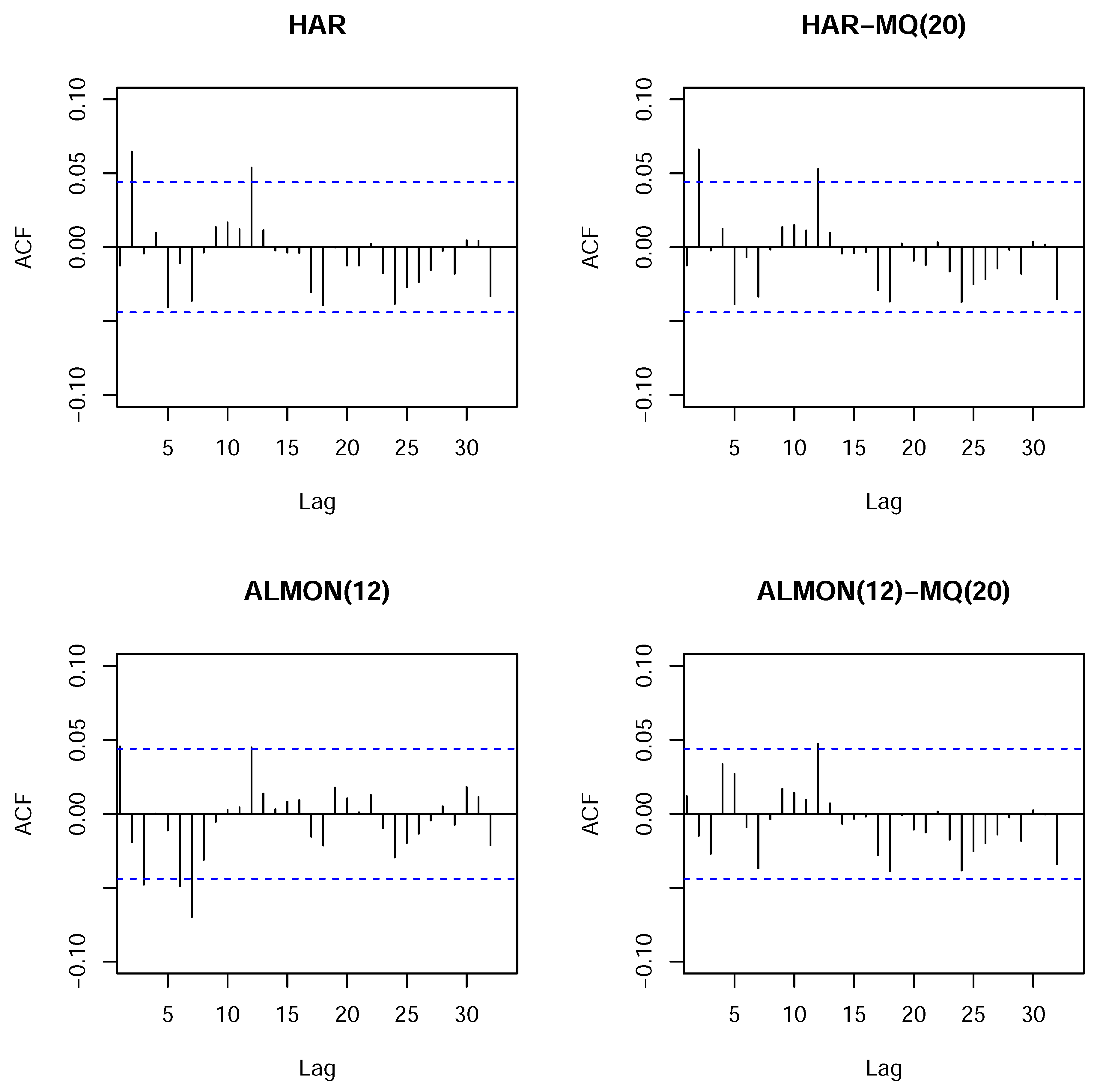
We use the AIC and BIC to select the relevant MQ terms, which mainly select the median as the relevant variable in most of the situations under consideration. Thus, we augment the linear models described above with a single term that corresponds to a moving median. Examples of estimated models and the corresponding auto-correlograms of the residuals are presented in Appendix C. In particular, the results for the estimated HAR, HAR-MQ(20), ALMON(12) and ALMON(12)-MQ(20) models are presented. The ordinary and nonlinear least squares estimators are used where appropriate to estimate the parameters. It should be noted that any configuration of the ALMON-MQ model always satisfies the sufficient stability condition defined in Proposition 1, whereas the results for other models vary (see Table C2 in Appendix C).
It can be seen from the results provided in Appendix C, for the models with the MQ term, that the moving median is always significant, whereas the third HAR term, which is connected with the monthly aggregate component, becomes insignificant whenever the moving median is added, as in the HAR-MQ(20) model. Furthermore, by considering the plots of the autocorrelation functions of the residuals in Figure C1 (see Appendix C), we can see that the presence of the moving median in the ALMON(12)-MQ(20) model removes a number of the spikes observed in the autocorrelation function of the residuals of the ALMON(12) model. However, in the case of the HAR model, the moving median is not able to remove the observed spikes of the autocorrelations at Lags 2 and 12. The same also holds for the HAR-MQ(12) model (unreported). These results are presented for samples 1–2,000. The results for samples that only comprised the first 1,000 observations and the whole dataset are not reported, but they are very similar and, correspondingly, have a bit less (or more) pronounced features discussed previously when the first 1,000 observations (or the whole dataset) is used.
It is relevant to recall that two lag orders can be selected in the models with MQs: the number of linear autoregressive terms and the number of periods used to calculate the MQs (window size). In general, the window size used for the MQ calculations might not coincide with the number of linear autoregressive terms. However, as noted in Section 2, MQs entail a representation with a certain linear part. As a result, unless the maximum lag of the MQ window is quite large, which would have the consequence of nearly negligible linear terms, we can expect to detect the required size of the moving window using the standard lag selection procedure based on a linear model. Indeed, whenever we used the information criteria to select the sub-sample window size from which the MQs are calculated, the criteria also indicate the 12 or 20 period window sizes for MQs in most situations, i.e., combinations of models, various MQ terms, maximum number of lags and different samples. 
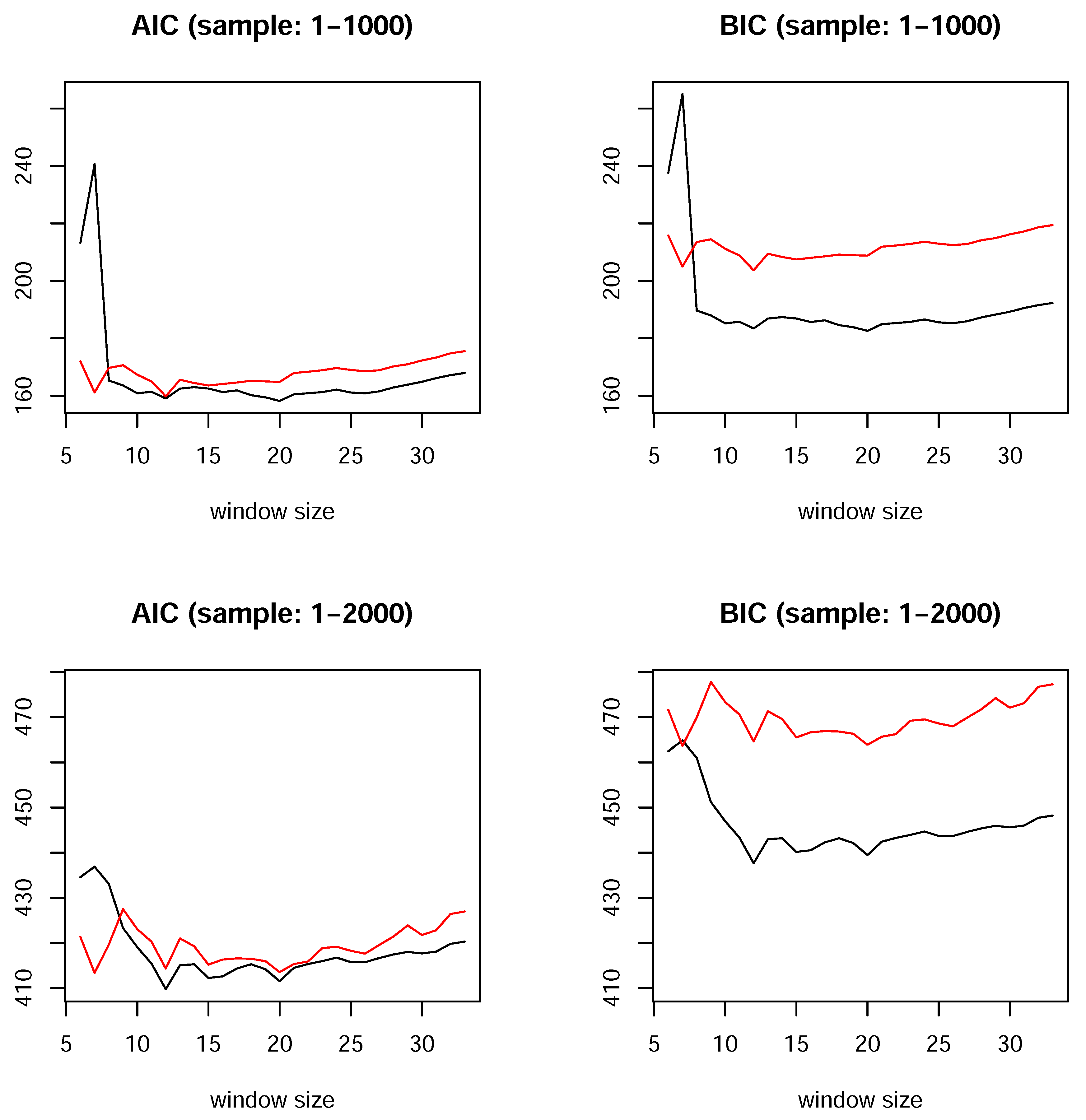
Figure 8 plots the AIC and BIC values for the ALMON model with a fixed number (twelve 9) of autoregressive terms, but a changing window size is used to calculate the MQs. The results are similar for the other models. The range of lags considered is 6–33, where the maximum is bounded by ( 10 log 10 T ) . The results are presented for sample sizes 1–1,000 and 1-2,000, and the two cases of MQs: (1) with all of the MQs present in the model (red line); and (2) only including the moving median (black line).
Figure 8. Effect of the moving window size, which is used to calculate the MQs, on the values of the information criteria for the ALMON(12) model with all MQs (red line) and only including the moving median (black line).
Econometrics 03 00002 g008
The information criteria are basically in agreement. First, the lowest value is obtained when only the moving median is used in all cases. Furthermore, they select 20 as the most informative window size for the moving median when the sample comprises the first 1,000 observations, whereas the criteria select 12 periods for the window size of the moving median when the sample comprises the first 2,000 observations. It is important to note that the dips in the values of the criteria at window sizes of 12 and 20 are observed with all samples.
Next, it is interesting to note that for both of the samples, the AIC and BIC figures show that the model with all of the MQs has a dip at a window size of seven. With this window size, the moving median is quite uninformative (the information criteria have large values), which may suggest that considering some other quantiles in addition to this window size could improve the model further. This was not attempted in the present study in order to keep the presentation compact and because the BIC strongly favors the case that includes a single moving median. Hence, we use it in the sequel as the most informative MQ to augment the linear autoregressive models.
All of the results described above are obtained using only the in-sample data without observations 2,001–3,000. Table 3 characterizes the in-sample model selection results, i.e., the models among those considered that are suggested for use based on the information criteria. In each category, the numbers of the three most informative models are shown in bold, while the best in each category are underlined.
Table 3. Values of the information criteria based on the in-sample evaluation of models.
Sample:1–1,0001–2,000
Criterion:AICBICAICBIC
HAR161.1185.5422.7450.6
AR(12)167.2235.8423.2501.5
AR(20)175.7283.2432.0555.0
ALMON(12)167.2186.8435.8458.2
ALMON(20)162.8182.4429.9452.3
HAR-MQ(12)158.8188.2414.6448.2
HAR-MQ(20)162.3191.7418.7452.3
AR(12)-MQ(12)167.5240.9416.2500.2
AR(12)-MQ(20)164.2237.6417.8501.7
AR(20)-MQ(12)176.2288.6425.5554.1
AR(20)-MQ(20)177.1289.5429.2557.8
ALMON(12)-MQ(12)183.2207.7466.1494.1
ALMON(20)-MQ(12)179.3203.7461.9489.8
ALMON(12)-MQ(20)158.1182.5411.3439.2
ALMON(20)-MQ(20)212.0236.4522.3550.3
Note: In each category, the numbers of the three most informative models are shown in bold, while the best in each category are underlined.
The HAR model performs well, and it is among the best three models in three out of four cases. However, the ALMON(12)-MQ(20) model is not only among the best three models, but also the best in three out of four cases. Furthermore, in the case where it performs second best, the BIC value differs only marginally from that of the best model. Thus, the ALMON(12)-MQ(20) model appears to have a good chance of being selected a priori (using the in-sample data) as a suitable candidate for further usage/forecasting.
Let us consider the out-of-sample forecasting evaluation of the models. The maximum lag order does not vary in the HAR, i.e., it is fixed at 20; thus, we set the HAR model precision as a benchmark in the relative forecasting performance evaluation. Table 4 shows the relative out-of-sample mean squared forecasting errors for the models characterized above. Table D1 and Table D2 in Appendix D also contain analogous results for the mean absolute percentage error (MAPE) and the mean absolute scaled error (MASE) criterion, which is favored by [63]. The qualitative results are unchanged.
Table 4. Relative out-of-sample forecasting precision (the benchmark is the mean squared forecasting error of the HAR model in each case). Index: S&P 500 (live). Initial series: realized variance (RV). Transformation: log 100 252 R V t . Forecasting horizon: one day.
Initial Estimation Sample:1–1,0001–1,0001–2,000
Initial Forecast Sample:1,001–2,0001,001–3,0002,001–3,000
Type of Forecast:FixedRecursiveRollingFixedRecursiveRollingFixedRecursiveRolling
HAR1.0001.0001.0001.0001.0001.0001.0001.0001.000
AR(12)1.0021.0011.0010.9990.9950.9960.9930.990 *0.989 *
AR(20)1.0081.0071.0121.0020.9981.0030.990 *0.9900.993
ALMON(12)1.0181.0060.9991.0010.9950.9930.987 *0.986 *0.986 *
ALMON(20)1.0141.0050.9980.9990.9940.992 *0.987 *0.986 *0.986 *
HAR-MQ(12)0.9960.9950.9961.0021.0011.0011.0091.0051.005
HAR-MQ(20)0.996 **0.996 *0.9950.997 **0.9990.9991.0011.0011.002
AR(12)-MQ(12)0.9950.9950.9950.9990.9950.9981.0030.9950.995
AR(12)-MQ(20)0.9980.9990.9990.9970.993 *0.9950.9920.989 *0.988 *
AR(20)-MQ(12)1.0031.0011.0071.0020.9981.0051.0000.9960.999
AR(20)-MQ(20)1.0041.0041.0091.0000.9971.0030.9910.9910.995
ALMON(12)-MQ(12)0.9940.9900.987 **0.9940.991 *0.988 **0.9960.9910.989
ALMON(20)-MQ(12)0.9930.9900.987 **0.9930.990 *0.987 **0.9960.9910.990
ALMON(12)-MQ(20)0.9920.9920.988 **0.987 ***0.987 ***0.985 ***0.985 **0.983 **0.983 **
ALMON(20)-MQ(20)0.9920.9920.988 **0.987 ***0.987 ***0.984 ***0.985 **0.983 **0.983 **
Note: The numbers of the two best performing models in each category are shown in bold. The models that consistently outperform the HAR model in all of the situations considered are underlined. The cases rejected significantly at the 10%, 5% and 1% levels, given the null hypothesis of equality to the HAR forecasting precision, are indicated by *, ** and ***, respectively. The [64] test is applied with a squared-error loss function.
Let us take a look at the results presented in Table 4. The numbers greater than one show that a model under consideration is inferior to the HAR in terms of the forecasting precision. The numbers shown in bold indicate the two models that perform best in each category in terms of the precision. In addition, the cases are indicated where the hypothesis of equal performance, in comparison with the HAR model, is rejected significantly using the [64] test 10, such that the forecast precision of a model under consideration is not equivalent to the HAR model (in favor of the alternative that the mean squared forecasting error of a model under consideration is less than that of the HAR forecast).
It can be seen that the relative performance of the unrestricted linear and ALMON models is mixed compared with the HAR model. When the initial estimation sample size is 1,000, they are outperformed by the HAR model in most cases, but for a larger sample size of 2,000 observations, the unconstrained autoregressions and the ALMON model yield better (and sometimes significantly better) precision, which is consistent with the findings in [56].
When the ALMON model is augmented with the moving median term, it outperforms all of the models under consideration, and in many cases, it also leads to the rejection of the hypothesis that its forecasting performance is equal to that of the HAR model. The moving median window of size of 20 appears to produce the best (or very close to the best) performance in all cases. However, even using a window size of 12, which equals the number of terms favored by the information criteria in the ALMON and unconstrained linear autoregression models (without MQs), produces a very similar performance. It should be noted that these models belong to a set of five models (underlined in Table 4) that consistently outperform the HAR model in all of the situations considered (samples and types of forecasting).
We recall that the ALMON(12)-MQ(20) model was favored by the information criteria in the in-sample analysis. Hence, this precision would have been realized in practice if the standard model selection procedures were employed as described previously. Thus, we can conclude that MQs were not only significant in the in-sample analysis, but that they also were relevant for the improvement of the out-of-sample forecasting precision.

5. Robustness and Extensions

In this section, we first present various sensitivity analyses using the S&P 500 index considered until now with the best (AR-MQ) model developed in the previous section. Afterwards, we extend the scope of analysis by: (1) allowing for some larger MQ window sizes than the window sizes up to 33 lags, as defined by the rule 10 log 10 T that we previously considered; (2) considering more indices from the Oxford-Man Institute database; and (3) testing for neglected non-linearity using the MQ and RESET tests using the latest available dataset from the Oxford-Man Institute.

5.1. Sensitivity of S&P 500 Analysis

In this subsection, we are interested in whether the presented findings are sensitive to some deviations from the previously considered situation in terms of the volatility measure, forecasting horizon, the usage of the logarithmic transformation of RV and the length of the window (sample size) used to estimate the parameters of the models. It should be pointed out that in all of these illustrations of robustness, we re-estimated the parameters using the respective new data, but with the models having the same specifications used in Table 4 without checking whether these models were the most informative given the new data, as well as without taking into consideration that the residuals of the multi-step forecasting models and of models without logarithmic transformation of the data depart severely from the white noise assumption.
We start from the change of the employed measure of volatility. Namely, until this point, the initial series that we used was the realized variance from the Oxford-Man Institute of Quantitative Finance dataset, but the analogous result would also hold when, for example, the realized kernel is used as an initial series (see Table E1 in Appendix E, where a one day ahead relative forecasting precision is presented, which is analogous to Table 4). All of the features identified using the logarithm of realized variance series remain, and the ALMON-MQ models are the best ones in terms of the out-of-sample forecasting.
We previously concentrated on a comparison of a single day ahead forecasting performance, but similar results are observed with more distant forecasts. Table E2 in Appendix E reports the relative precision of the forecasting of realized volatility over a weekly period using an analogous representation to that in Table 4. Here, again, the ALMON(12)-MQ(20) and ALMON(20)-MQ(20) models are the best-performing and consistently outperform the HAR model in all of the situations considered (underlined). However, an interesting feature appears that all of the other models, which include the moving median with a window of size of 20 periods, also become consistently better than the HAR model. On the other hand, the specifications of ALMON-MQ with the moving median with a window of a size of only 20 periods become much less precise. It seems therefore that longer past horizons might start to matter more whenever forecasting over longer future periods are of interest.
Relying on the observations that the logarithm of realized variance is much closer to normality and less heteroscedastic than that without such a transformation, we previously considered the logarithmically transformed series. However, similar findings are obtained when the logarithmic transformation is not applied (see Table E3 in Appendix E). Namely, in most of the situations, the ALMON(12)-MQ(12) and ALMON(12)-MQ(20) remain the best-performing models. However, in one of the considered cases of samples, the forecasting precision produced by the HAR-MQ(20) is the best one instead.
Finally, we evaluate the usage of shorter samples to estimate the parameters of the models. It can be expected that a shorter estimation period allows the models to be more adaptive to the varying volatility, and the standard HAR could perform relatively well. The results related to the sample sizes of 125, 250 and 500 observations instead of the previously used 1,000 and 2,000 observations are summarized in Table E4 in Appendix E. The previously established features apply also whenever the sample of observations is reduced to 500 (see the fixed and rolling cases only, since in the recursive type of forecasting, the number of observations increases with the sample). Whenever the number of observations, used to estimate the models, reduces further to 250 and 125, other models start appearing among the best-performing ones. This can come from two sources. First, in shorter samples, coefficients of the models become more adaptive to the changing process of volatility, thus eliminating the need for describing the low-frequency fluctuation component in the level of volatility. Second, much shorter samples create huge inefficiency of the estimator of MQ parameters, as was revealed in Subsection 3.4. It is rather remarkable that even with the samples of 250 observations, the MQ effects seem to be still helping to improve the forecasting precision.
To summarize the findings, the results are quite robust in these new situations, whenever the estimation sample sizes are reasonable. Especially, the relevance of the moving median in producing more precise forecasts is retained.

5.2. Relevance of Larger MQ Windows for S&P 500

As was identified in Section 3.4, in the presence of larger window sizes of MQs, much larger samples are required relative to the window of MQs in order to get a satisfactory estimation precision. For the linear autoregressions, it is also unlikely to have precise parameter estimates with, e.g., 100 or 200 parameters, even in samples of several thousand of observations. Hence, we do not strive for any sophistication in introducing larger window sizes, but rely on the “parsimony” argument similar to [30] and consider further “parsimonious” periods. Namely, we augment the previously developed AR(12)-MQ(20), which was the best model in most of the considered situations, with the MQ terms having windows of three and six months (namely, 60 and 120 days). We use the quartiles as the MQ terms (the usage of the other structure of quantiles does not change the qualitative picture). Table 5 reports the in-sample findings, where only the significant quantiles are kept in the extended AR-MQ models. For comparison purposes, we also include the previously used ALMON(12)-MQ(20) model containing only the moving median term.
As can be seen, whenever the three-month MQ window is used, only the third quartile ( q 0 . 75 ( 60 ) ) is left as significant in the model. Hence, the quite extreme, but not the most extreme, observations over this period seem to leave an imprint. However, the information criteria give little support to such an extension 11, despite that the added MQ term seems to be statistically significant. On the other hand, whenever the six-month MQ window is used (either separately or augmenting the three-month window period), only the maximum term ( q 1 ( 120 ) ) remains significant. It seems therefore that the longer periods of MQ terms are quite relevant in explaining volatility, and the spikes of volatility have an influence on the market development for quite a long time.
The out-of-sample forecasting performance of these models will be evaluated next using an extended set of indices from the Oxford-Man Institute database.
Table 5. Estimated models: ALMON(12)-MQ(20) and its extensions (estimation sample: 1–2,000).
Coefficients Extensions
noneq 0.75 (60)q 1 (120)
Intercept 0.1239 *** 0.0812 * 0.0664
( 0.0405 ) ( 0.0459 ) ( 0.0451 )
of ALMON restriction: ψ 0 0.7205 *** 0.7317 *** 0.7222 ***
( 0.0469 ) ( 0.0484 ) ( 0.0487 )
ψ 1 0.5960 *** 0.5814 *** 0.5813 ***
( 0.0701 ) ( 0.0605 ) ( 0.0710 )
of MQ terms:
q 0.5 ( 20 ) (moving median, window=20) θ 1 0.2310 *** 0.1478 ** 0.1711 ***
( 0.0476 ) ( 0.0621 ) ( 0.0532 )
q 0.75 ( 60 ) (moving 3rd quartile, window=60) θ 2 0.0824 **
( 0.0381 )
q 1 ( 120 ) (moving maximum, window=120) θ 3 0.0592 ***
( 0.0213 )
Standard error of residuals 0.26800.26850.2668
Degrees of freedom 1,9771,9361,876
AIC 411.279411.289375.117
BIC 439.236444.715408.354
i = 1 3 | θ i | + j = 1 12 | β j | 0.95140.96190.9524
Note: Standard errors of coefficients are reported in parentheses with *, ** and *** indicating the significance at the 10%, 5% and 1% levels, respectively. { β j } j = 1 k are defined as in Equation (15) for the ALMON ( k = 12 ) model. The sufficient stability condition defined in Proposition 1 requires i = 1 3 | θ i | + j = 1 12 | β j | < 1 to hold.

5.3. Out-of-Sample Forecasting Performance (for More Indices)

Let us now turn to the consideration of the out-of-sample forecasting performance of the previously developed models (developed for the realized volatility of S&P 500 index returns) whenever applied to the first seven indices 12 provided in the Oxford-Man Institute database described in Section 4. To save space, we present the results only of the rolling forecasting approach, which is preferable, given the possibility of the presence of structural breaks (see, e.g., [68]).
Since we use models with several quantiles and different windows, let us introduce an explicit definition of the cases under consideration in the names of the models. For instance, ALMON(12)-MQ(20:0.5; 60:0.75) will indicate that there are two window lengths used of 20 and 60 days with the median ( q 0 . 5 ) from the 20-day period and the third quartile ( q 0 . 75 ) from the 60-day period included.
Table 6 reports the out-of-sample forecasting MSE of the models under consideration relative to the MSE of the HAR model for the realized volatility of various indices.
Table 6. Relative out-of-sample forecasting precision (a benchmark is the mean squared forecast error of the HAR model in each case). Indices: seven different. Initial series: realized variance (RV). Transformation: log 100 252 R V t . Forecasting horizon: one day. Forecasting type: rolling. Initial estimation sample: 1–2,000.
ModelsIndices:
S&P 500FTSE 100Nikkei 225DAXRussell 2000AORDDJIA
HAR1.0001.0001.0001.0001.0001.0001.000
AR(12)0.989 *0.9940.9930.9950.984 *1.0020.991
AR(20)0.9930.9970.9960.9940.9851.0020.998
ALMON(12)0.986 *1.0180.9911.0030.9970.99 *0.985 **
ALMON(20)0.986 *1.0190.9911.0030.9960.988 **0.985 **
HAR-MQ(12)1.0051.0001.0001.0021.0061.0011.003
HAR-MQ(20)1.0021.0010.9960.9981.0001.0010.999
AR(12)-MQ(12)0.9950.9950.9940.9950.9901.0030.995
AR(12)-MQ(20)0.988 *0.9930.989 **0.9920.979 **0.9970.99 *
AR(20)-MQ(12)0.9990.9980.9970.9950.9931.0021.002
AR(20)-MQ(20)0.9950.9970.9920.9920.9851.0030.997
ALMON(12)-MQ(12)0.9891.0040.982 **0.9910.986 *0.9910.990
ALMON(20)-MQ(12)0.9901.0040.982 **0.9900.986 *0.988 **0.990
ALMON(12)-MQ(20)0.983 **1.0060.975 ***0.987 *0.979 ***0.984 ***0.983 ***
ALMON(20)-MQ(20)0.983 **1.0060.975 ***0.987 *0.979 ***0.987 **0.983 ***
ALMON(12)-MQ(20:0.5; 60:0.75)0.982 **1.0060.978 ***0.987 *0.976 ***0.983 **0.984 **
ALMON(20)-MQ(20:0.5; 60:0.75)0.982 **1.0060.978 ***0.987 *0.975 ***0.985 **0.984 **
ALMON(12)-MQ(20:0.5; 120:1)0.980 **1.0060.978 ***0.985 **0.975 ***0.985 **0.980 ***
ALMON(20)-MQ(20:0.5; 120:1)0.981 **1.0060.978 ***0.986 **0.975 ***0.986 **0.981 ***
Note: The numbers of the two best-performing models in each category are shown in bold. The model that consistently outperforms the HAR model in all of the situations considered is underlined. The cases rejected significantly at the 10%, 5% and 1% levels, given the null hypothesis of equality to the HAR forecasting precision, are indicated by *, ** and ***, respectively. The [64] test is applied with a squared-error loss function.
In all of the cases, but FTSE 100 (for which the best-performing model is the AR(12)-MQ(20)), the main features identified using the S&P 500 data regarding the AR-MQ models are retained. Namely, the AR-MQ models have smaller forecasting MSE relative to the HAR, and the difference is statistically significant.
The stable performance of the AR(12)-MQ(20) in terms of the HAR model (it should be pointed out that the AR(12)-MQ(20) precision is also consistently better than that of the AR(12) in all of the cases) implies that, even without imposing the restriction on the linear autoregressive part with the aim of getting more efficient estimation of the parameters, the moving median affects positively the forecasting precision of the unconstrained RV model. On the other hand, it can be observed that the usage of the ALMON restriction alone does not ensure the stable outperforming of the HAR model. The coupling of the two approaches (imposing an ‘adequate’ constraint and the usage of MQ terms) leads to the best-performing model.
In the case of FTSE 100, it can be observed that the ALMON models (without MQ terms) fail already in relative terms to the HAR model (although the additional usage of the MQ terms in ALMON-MQ softens this failure). Hence, it seems that the adequacy of an imposed constraint on the linear autoregressive part plays here a crucial role. In fact, although unreported in the table, the usage of, e.g., the HAR with the MQ(20:0.5, 120:1) terms yields a significant (at the 5% significance level) out-of-sample forecasting improvement over the HAR model for the FTSE 100. However, such a model performs less well for other indices and is therefore not included in Table 6.
The contribution of the longer-term MQ windows to the forecasting performance depends on the horizon and the indices. For the S&P 500, DAX, Russell 2000 and DJIA indices, the six-month moving maximum improves the precision, whereas for the AORD, the best performance is observed with the three-month moving third quartile. Hence, in the five out of seven cases under consideration, the forecasting performance was further improved by adding the longer spans of moving quantiles.

5.4. MQ and RESET Testing Results Using the Latest Available Dataset (for October 8, 2014)

Until now, we concentrated mostly on the out-of-sample forecasting value of the MQ terms by imitating the in- and out-of-sample modeling and forecasting procedure. However, as pointed out, e.g., in [69], whenever the testing or discrimination among models is performed, it is unreasonable to omit the available information, and the tests should be applied using the whole dataset. In this subsection, we therefore present the testing results for the significance of the MQ terms using the whole dataset. In fact, we use the latest dataset available for the moment of the revision of the paper from the Oxford-Man Institute of Quantitative Finance dated October 8, 2014. Such a choice is motivated by the fact that, whenever we used the 3,000 observations that were employed in the previous forecasting exercises, the results seemed to be too good 13.
Table 7 reports the heteroscedasticity-consistent testing results for the MQ test (as in Theorem 14 1) with three and five moving quantiles (min-med-max and quartiles, correspondingly). In light of the results of Subsection 3.6, we also present the testing results using the heteroscedasticity-consistent RESET tests. For the RESET tests and the linear autoregressive part of the MQ test, we consider k { 12 , 20 } , motivated by the information criteria and the HAR specification. For the MQ effects, we cover the lag windows of 20, 60 and 120, in connection with the previously performed analysis.
For the linear autoregression of order k = 12 , the null hypothesis of linearity is rejected at the 1% significance level using the MQ test in all cases, but one (for the DJIA with MQ 60 period window, the p-value is 0.013). For the linear autoregression of order k = 20 , the null hypothesis of linearity is rejected at the 5% significance level at least for some windows of MQs.
Aside from the Russell 2000 case, the linearity is rejected using the MQ test at (considerably) smaller significance levels, and the RESET tests are often insignificant (at the 5% significance level say), especially whenever the linear autoregression of order k = 20 is under consideration. In the cases of Russell 2000, the presence of other non-linearities against which the MQ test has smaller power than the RESET tests seems to be very likely. For the DJIA, DAX and S&P 500, the possibility of a Markov regime-switching GARCH process, which leads to powerful MQ and less powerful RESET tests, is also probable.
Table 7. Heteroscedasticity robust p-values of the MQ and RESET testing (for neglected non-linearity).
AR Order Under H0Test SpecificationIndices:
S&P 500FTSE 100Nikkei 225DAXRussell 2000AORDDJIA
k = 12 MQ(20: 0,0.5,1)0.0020.0020.0010.0000.0020.0030.001
MQ(60: 0,0.5,1)0.0010.0000.0100.0010.0000.0000.004
MQ(120: 0,0.5,1)0.0000.0000.0010.0000.0010.0000.000
MQ(20: 0,0.25,0.5,0.75,1)0.0050.0000.0060.0000.0020.0100.001
MQ(60: 0,0.25,0.5,0.75,1)0.0050.0000.0080.0020.0020.0000.013
MQ(120: 0,0.25,0.5,0.75,1)0.0000.0000.0030.0030.0060.0000.001
RESET(2)0.0480.8630.3480.0680.0000.2480.018
RESET(2:3)0.0400.0450.5240.0140.0010.3110.005
RESET(2:4)0.0800.0900.6910.0310.0020.4660.011
k = 20 MQ(20: 0,0.5,1)0.0120.0090.2980.0010.0220.5350.007
MQ(60: 0,0.5,1)0.0350.0010.1210.1320.0240.0000.071
MQ(120: 0,0.5,1)0.0010.0030.0120.0260.0370.0040.002
MQ(20: 0,0.25,0.5,0.75,1)0.0320.0310.5480.0070.0420.6670.008
MQ(60: 0,0.25,0.5,0.75,1)0.0760.0050.0850.1670.0870.0020.133
MQ(120: 0,0.25,0.5,0.75,1)0.0030.0120.0310.0840.1030.0030.008
RESET(2)0.0550.7070.3040.0630.0010.2490.025
RESET(2:3)0.0580.1060.4910.0290.0020.3530.010
RESET(2:4)0.1120.1910.6600.0610.0050.5150.024
Note: Figures in bold highlight the cases where the linearity is rejected at the 5% significance level, and the red ones highlight the cases where the rejection is at the 1% significance level.

6. Final Remarks

The non-linear autoregression model with MQs in the DGP introduced in this paper can produce realizations looking as if they have both the structural breaks and the long-memory pattern. Such features are often observed in empirical data. Hence, it seems to be important to test using the proposed instruments whether the observed ‘persistence’ and ‘structural breaks’ cannot be caused by the presence of moving quantiles.
The presented simulations reveal that, in order to obtain the satisfactory precision of estimates and the possibility to draw conclusions using the limiting distribution of the tests, much larger samples than the (unknown) window of moving quantiles is required. Provided that such a ‘memory window’ of the historical characteristics is relatively lengthy, the most likely detection of the proposed effects can be expected in financial data. It is less likely to be detected in macroeconomic process, unless the relevant ‘memory window’ of MQs were much shorter.
The preformed simulations also revealed that the RESET tests fail to detect the moving quantiles’ non-linearity, irrespective of orders used for the testing. Since the RESET tests have power against many other non-linearities, the significance of the MQ test and insignificance of the RESET tests can be a useful indicator that the MQ modeling could be relevant.
In the empirical illustration of the application of the proposed model, we showed that the moving quantiles improve the forecasting precision of the realized volatility. Further, relative precision gains can be expected by considering more complicated structures of moving quantiles, possibly with time-varying window sizes, lagging effects, etc. Similar to [70], the importance of other exogenous variables (and their MQs) could be explored, as well as more complex nonlinearity structures, e.g., allowing for interactions, asymmetries, etc. However, these extensions would require further development of the underlying theoretical framework.
For the S&P 500 index, it is interesting to note that not only the ALMON-MQ models outperformed the benchmark in all cases, but also the relative precision of these models was even better during the out-of-sample periods (1,000–3,000 and 2,000–3,000), which included the more volatile period of observations 2,000–3,000. This finding is similar to that reported by [70], who used a different nonlinear model with exogenous explanatory variables.
Based on the simple case considered in this study, we can obtain an interesting interpretation of the result that the moving median was the most informative variable among the MQs considered. As the moving median is a robust filter, this suggests that the participants in the financial market might also value/respond to a robust measure of recent volatility. Since we found that these effects become more relevant during more volatile periods, this might suggest that the markets during high volatility become or are considered to be noisy, and therefore, more robust measures become more relevant. This finding appears to provide an important new feature that augments the usual philosophy underlying the models of conditional heteroscedasticity.
On the other hand, the significance of longer ‘parsimonious’ periods of MQ terms also point to the fact that the extreme levels of volatility reached within, e.g., half a year remain remembered and result in a somewhat higher volatility level thereafter during this period. Apart from a general increase of uncertainty induced by some excess periods of volatility, it might be the case that some market participants do not close their (unfavorable) open positions whenever some shocks occur in the market, causing higher volatility periods. They wait instead for some ‘parsimonious’ period, which depends on their financial resources and the size of open positions, for a more favorable situation and an opportunity to close the position without a (or with a smaller) loss.
The fact that the best results are often obtained for models where the exponential Almon restriction and the MQ terms are present can shed light on the contributions from two different components (similar to the idea presented in [44]). The exponential Almon restriction imposes an exponential decay of the autoregressive effects and can reasonably model only the very short memory effects; whereas the usage of moving quantiles seems to capture the development in the lower frequency component. However, other than in [44], this low frequency component in our model has an endogenous nature.
The established findings seem to be quite robust in various sensitivity analyses. Even using the specifications developed for the S&P index, the main features remain observable for several other considered indices. Furthermore, the empirical application of the MQ and RESET tests using the latest available dataset also indicates that the MQ effects are very likely to be present in a number of the considered realized volatility series. Therefore, it seems that our simple illustration of the usage of AR-MQ models could also have some value.

Acknowledgments

We thank the two reviewers for their valuable contribution in shaping our manuscript. We also greatly acknowledge the suggestions to our previous versions of the manuscript made by Timo Teräsvirta, Hidehiko Ichimura and Ser-Huang Poon, as well as other participants of the conferences (FindEcon 2012, Asian Meeting of the Econometric Society 2012, the 7th International Conference on Computational and Financial Econometrics) and seminars (at the University of Southern Denmark and the Center for the Study of Finance and Insurance, Osaka University). This work was partially supported by the JSPS Grants-in-Aid for Scientific Research No. 22243021 and No. 25245034.

Author Contributions

The authors contributed jointly to the paper.

Appendix

A. Proofs

Proof of Proposition 1. 
Starting from model in Equation (1) and using Equation (2), we obtain:
h ( x k , t - 1 ) : = c + ϕ x k , t - 1 + θ q m , t - 1 = c + j = 1 k ( ϕ j + θ j , t ) x t - j
and:
| h ( x k , t - 1 ) | | c | + j = 1 k | a j , t | | x t - j | , a j , t : = ϕ j + θ j , t
Using the explanation of θ j , t given in Equation (2) and noting that for each fixed t and i = 1 , 2 , , m , it holds that 1 I i , j , t = 1 1 I i , r , t = 0 , r j , we obtain:
j = 1 k | θ j , t | = j = 1 k i = 1 m θ i 1 I i , j , t δ i , j , t i = 1 m | θ i | j = 1 k 1 I i , j , t δ i , j , t = i = 1 m | θ i | max j δ i , j , t i = 1 m | θ i |
where the last inequality follows because of δ i , j , t [ 0 , 1 ] .
Hence,
j = 1 k | a j , t | = j = 1 k | ϕ j + θ j , t | j = 1 k | ϕ j | + j = 1 k | θ j , t | | | ϕ | | 1 + | | θ | | 1
Since, the linear function is also bounded on compacts, E | ξ t | < , and the error term has an absolutely continuous distribution with a density positive almost everywhere by assumption, the geometric ergodicity of the model-related Markov chain follows from [34], provided | | ϕ | | 1 + | | θ | | 1 < 1 . Then, Theorem 2.2 of [33] delivers the necessary result for the existence of a strictly stationary (causal) solution. ☐
Proof of Proposition 2. 
Since E | ξ t | r < is assumed, based on Theorem 2 in [40], it is necessary to show that there exist a positive number 0 < ρ < 1 and a constant c ¯ > 0 , such that:
| h ( x k , t - 1 ) | ρ max j { 1 , 2 , , k } | x t - j | + c ¯
However, this follows in a straightforward manner from inequality defined in Equation (A1) and Equation (A2), by letting ρ : = j = 1 k | a j , t | < ϕ 1 + θ 1 and c ¯ : = | c | . ☐
Proof of Proposition 3. 
Recall from Proposition 1 and Remark 1 that { x t } and { q t ( i ) } , i = 1 , 2 , , m , are stationary and ergodic sequences. Since, by definition, | q t - 1 ( i ) | j = 1 k | x t - j | , i = 1 , 2 , , m , based on the Minkowski inequality and stationarity of { x t } , we obtain, for a fixed k and r 1 ,
E | q t - 1 ( i ) | r j = 1 k E | x t - j | r 1 r r k r E | x t | r , i = 1 , 2 , , m
The Cauchy–Schwarz inequality also yields E | q t - 1 ( i ) x t - j | E | q t - 1 ( i ) | 2 E | x t - j | 2 for each i , j , t . Hence, E ξ t 2 < and Proposition 2 imply that C : = E z t z t < .
For a fixed k, let T k : = T - k . Let us note that E z t ξ t = E z t E ξ t | z t = 0 and z t ξ t is also a stationary and ergodic sequence, due to, for example, Proposition 3.36 in [71]. Hence, based on the Slutsky, continuous mapping and ergodic theorems (see, e.g., [72]), we have:
η ^ - η = 1 T k t = k + 1 T z t z t - 1 1 T k t = k + 1 T z t ξ t 0 k + m + 1
as T a.s.
To prove the remaining second part, consider:
σ ξ - 1 t = k + 1 T z t z t 1 2 η ^ - η = σ ξ - 1 1 T k t = k + 1 T z t z t - 1 / 2 1 T k t = k + 1 T z t ξ t
Since, for a given k, 1 T k t = k + 1 T z t z t C as T a.s., for the analysis of the convergence of the distribution, consider:
d T : = σ ξ - 1 C - 1 / 2 1 T k t = k + 1 T z t ξ t
Let us note that for F t = { x s , ξ s } s t , E z t ξ t | F t - 1 = 0 k + m + 1 and E ξ t 2 z t z t | F t - 1 = σ ξ 2 z t z t . Hence, Var T k - 1 / 2 t = k + 1 T z t ξ t = Var z t ξ t = σ ξ 2 C . As a result, E d T = 0 k + m + 1 and E d T d T = I k + m + 1 .
These results combined with those derived in the first part of the proof ensure the conditions needed for Theorem 5.25 in [71]; thus, the result follows. ☐
Proof of Theorem 1. 
Using Equation (10) and Equation (11) and noting that M H = H because of the idempotency of M, it follows that:
θ ^ H H θ ^ / σ ξ 2 = u ^ H H H - 1 H u ^ / σ ξ 2 = M ξ + H θ H H H - 1 H M ξ + H θ / σ ξ 2 = ξ H H H - 1 H ξ / σ ξ 2 + θ H H θ + 2 ξ H θ / σ ξ 2 = ζ ζ + D ( θ )
where:
D ( θ ) : = θ H H θ + 2 ξ H θ / σ ξ 2
and:
ζ : = σ ξ - 1 H H - 1 / 2 H ξ
Since, under H 0 : θ = 0 m , the autoregressive process is stationary and ergodic provided the conditions given in the theorem are satisfied, the ζ a N 0 m , I m can be established along the same lines as in Proposition 3.
Therefore, under H 0 : θ = 0 m , the claimed distribution of the test statistic is obtained asymptotically, whereas under H 1 : θ 0 m , the test statistic diverges because of θ H H θ / σ ξ 2 a.s. . ☐
Proof of Remark 3. 
After using the corresponding definitions presented just before Remark 3, the proof is analogous to that of Theorem 1. ☐

B. Additional Results from the Simulations

Figure B1 shows the Q–Q plots and distribution of the realizations of the AR-MQ model.
Figure B2 shows the power in finite samples of the MQ test against non-linearities N1–N8 (from the N block in Table 1).
Figure B3 shows the absent power of the MQ test against non-linearities N9–N14 (from the N block in Table 1).
Figure B1. The Q–Qplots (sample quantiles versus the theoretical ones) of 2,000 realizations of the AR-MQ model (with the moving maximum from the indicated window sizes k) and the (non-parametrically estimated) density of the standardized realization of the case with k = 60 (bottom right).
Econometrics 03 00002 g009
Note: It should be pointed out that some observed variability comes from the realized sample effects, which disappears with the usage of, e.g., 10,000 observations.
Figure B2. Distribution of empirical sizes of the MQ test for the data generated by the non-linear processes N1–N8 (DGPs from the N block in Table 1).
Econometrics 03 00002 g010
Figure B3. Distribution of empirical sizes of the MQ test for the data generated by the non-linear processes N9–N14 (DGPs from the N block in Table 1).
Econometrics 03 00002 g011

C. Examples of Estimated Models for the S&P 500 Index Returns (Estimation Sample: 1–2,000)

Table C1. Examples of selected estimated models (estimation sample: 1–2,000).
Coefficients Models
HARHAR-MQ(20)ALMON(12)ALMON(12)-MQ(20)
Intercept 0.1399 *** 0.1249 *** 0.1788 *** 0.1239 ***
( 0.0402 ) ( 0.0396 ) ( 0.0422 ) ( 0.0405 )
of HAR restriction: ψ 1 0.2541 *** 0.2535 ***
( 0.0308 ) ( 0.0309 )
ψ 2 0.4712 *** 0.4755 ***
( 0.0508 ) ( 0.0503 )
ψ 3 0.2196 *** - 0.1231
( 0.0423 ) ( 0.1555 )
of ALMON restriction: ψ 1 0.9296 *** 0.7205 ***
( 0.0167 ) ( 0.0469 )
ψ 2 0.3965 *** 0.5960 ***
( 0.0321 ) ( 0.0701 )
of moving medianθ 0.3453 ** 0.2310 ***
( 0.1501 ) ( 0.0476 )
Standard error of residuals 0.26880.26850.26970.2680
Degrees of freedom 1976197519851977
AIC 422.655418.750435.775411.279
BIC 450.609452.295458.155439.236
| θ | + j = 1 k | ϕ j | 0.94481.13580.92960.9514
Note: Standard errors of the coefficients are reported in parentheses, where *, ** and *** indicate significance at the 10%, 5% and 1% levels, respectively. { ϕ j } j = 1 k are defined as in Equation (14) and Equation (15) for the HAR ( k = 20 ) and ALMON ( k = 12 ) models, respectively. The sufficient stability condition defined in Proposition 1 requires that | θ | + j = 1 k | ϕ j | < 1 holds.
Table C2. Prevalence of the sufficient stability condition defined in Proposition 1 for the estimated models with MQ terms.
Estimation Sample
1–1,0001–2,0001–3,000
HAR-MQ(12)+++
HAR-MQ(20)+
AR(12)-MQ(12)
AR(12)-MQ(20)+++
AR(20)-MQ(12)
AR(20)-MQ(20)
ALMON(12)-MQ(12)+++
ALMON(20)-MQ(12)+++
ALMON(12)-MQ(20)+++
ALMON(20)-MQ(20)+++
Note: “+” denotes that a sufficient stability condition defined in Proposition 1 is satisfied. “–” indicates that it is not. Models that satisfy the condition in any sample are underlined.
Figure C1. The empirical autocorrelation functions (ACF) of the residuals of the estimated models: HAR (left-top), HAR-MQ(20) (right-top), ALMON(12) (left-bottom) and ALMON(12)-MQ(20) (right-bottom).
Econometrics 03 00002 g012

D. Out-of-Sample Forecasting Precision: MAPE (Table D1) and MASE (Table D2)

Table D1. Relative out-of-sample forecasting precision (the benchmark is the mean absolute percentage error (MAPE) of the HAR model in each case). Index: S&P 500 (live). Initial series: realized variance (RV). Transformation: log 100 252 R V t . Forecasting horizon: one day.
Initial Estimation Sample:1–1,0001–1,0001–2,000
Initial Forecast Sample:1,001–2,0001,001–3,0002,001–3,000
Type of Forecast:FixedRecursiveRollingFixedRecursiveRollingFixedRecursiveRolling
HAR1.0001.0001.0001.0001.0001.0001.0001.0001.000
AR(12)1.0001.0001.0011.0010.9970.9970.9970.993 *0.992
AR(20)1.0011.0011.0011.0010.9971.0000.9950.993 **0.995
ALMON(12)1.0121.0030.9991.0030.9970.995 *0.9900.991 *0.990 *
ALMON(20)1.0091.0010.9981.0010.9960.994 *0.9910.991 *0.991 *
HAR-MQ(12)0.997 *0.997 *0.9981.0000.9990.9991.0041.0021.001
HAR-MQ(20)0.9980.9990.9990.998 *0.9990.9990.9990.9990.998
AR(12)-MQ(12)0.9960.9960.9980.9980.995 *0.9961.0000.9940.992
AR(12)-MQ(20)0.9970.9991.0000.9990.996 *0.9960.9950.992 **0.992 **
AR(20)-MQ(12)0.9980.9980.9981.0000.9960.9990.9980.9930.996
AR(20)-MQ(20)0.9991.0011.0000.9990.9950.9990.9920.989 **0.991 *
ALMON(12)-MQ(12)0.9960.994 *0.994 *0.995 *0.993 **0.992 **0.9940.991 *0.990 **
ALMON(20)-MQ(12)0.995 *0.994 *0.994 *0.994 **0.992 **0.992 **0.9940.991 *0.990 **
ALMON(12)-MQ(20)0.993 *0.9950.995 *0.990 ***0.992 ***0.992 ***0.987 ***0.988 ***0.988 ***
ALMON(20)-MQ(20)0.993 *0.9950.995 *0.990 ***0.992 ***0.992 ***0.989 ***0.988 ***0.988 ***
Note: The numbers of the two best-performing models in each category are shown in bold. The models that consistently outperform the HAR model in all of the situations considered are underlined. The cases rejected significantly at the 10%, 5% and 1% levels given that the null hypothesis implies equality to the HAR forecasting precision are indicated by *, ** and ***, respectively. The [64] test is applied with an absolute error loss function.
Table D2. Relative out-of-sample forecasting precision (the benchmark is the mean absolute scaled error (MASE) of the HAR model in each case). Index: S&P 500 (live). Initial series: realized variance (RV). Transformation: log 100 252 R V t . Forecasting horizon: one day.
Initial Estimation Sample:1–1,0001–1,0001–2,000
Initial Forecast Sample:1,001–2,0001,001–3,0002,001–3,000
Type of Forecast:FixedRecursiveRollingFixedRecursiveRollingFixedRecursiveRolling
HAR1.0001.0001.0001.0001.0001.0001.0001.0001.000
AR(12)0.9981.0001.0011.0000.9960.9960.9970.9930.991
AR(20)0.9991.0021.0021.0000.9970.9990.9950.9920.994
ALMON(12)1.0061.0000.9970.9990.9960.9950.9930.9920.992
ALMON(20)1.0040.9990.9960.9980.9950.9940.9930.9920.992
HAR-MQ(12)0.9960.9960.9981.0001.0001.0001.0051.0031.002
HAR-MQ(20)0.9990.9990.9990.9991.0001.0001.0011.0001.000
AR(12)-MQ(12)0.9940.9950.9970.9990.9950.9961.0020.9950.993
AR(12)-MQ(20)0.9971.0001.0010.9990.9960.9960.9960.9920.991
AR(20)-MQ(12)0.9960.9980.9981.0000.9961.0001.0000.9940.996
AR(20)-MQ(20)0.9981.0011.0010.9990.9950.9990.9940.9900.991
ALMON(12)-MQ(12)0.9940.9930.9930.9940.9930.9920.9960.9930.991
ALMON(20)-MQ(12)0.9930.9920.9920.9930.9920.9920.9960.9930.992
ALMON(12)-MQ(20)0.9930.9950.9950.9900.9920.9910.9890.9880.988
ALMON(20)-MQ(20)0.9930.9950.9950.9900.9920.9910.9890.9880.988
Note: The numbers of the two best-performing models in each category are shown in bold. The models that consistently outperform the HAR model in all of the situations considered are underlined.

E. Robustness Analysis

Situations under consideration:
Table E1 shows the forecasting results with the realized kernel (RK) estimator of volatility.
Table E2 shows the forecasting results over a week ahead.
Table E3 shows the forecasting results without logarithmic transformation.
Table E4 shows the forecasting with sample sizes of 125, 250 and 500 observations.
Table E5 shows the forecasting results for the DJIA index.
Table E1. Relative out-of-sample forecasting precision (the benchmark is the mean squared forecast error of the HAR model in each case). Index: S&P 500 (live). Initial series: realized kernel (RK). Transformation: log 100 252 R K t . Forecasting horizon: one day.
Initial Estimation Sample:1–1,0001–1,0001–2,000
Initial Forecast Sample:1,001–2,0001,001–3,0002,001–3,000
HAR1.0001.0001.0001.0001.0001.0001.0001.0001.000
AR(12)0.9990.9991.0000.9980.9950.9970.9920.9910.990
AR(20)1.0061.0051.0091.0000.9981.0030.989 *0.9910.993
ALMON(12)1.0201.0081.0021.0040.9980.9980.9880.9880.988
ALMON(20)1.0171.0071.0011.0030.9970.9970.9890.9890.988
HAR-MQ(12)0.9980.9980.9981.0031.0011.0011.0071.0041.004
HAR-MQ(20)1.0000.9990.9981.0000.9991.0000.9991.0001.000
AR(12)-MQ(12)0.9920.9950.9970.9970.9950.9981.0010.9960.996
AR(12)-MQ(20)1.0010.9991.0010.9990.9940.9970.991 *0.990 *0.989 *
AR(20)-MQ(12)1.0001.0021.0060.9990.9981.0040.9970.9950.998
AR(20)-MQ(20)1.0071.0051.0081.0000.9971.0030.9880.9900.993
ALMON(12)-MQ(12)0.9930.9920.990 *0.9930.991 *0.989 **0.9930.9890.988 *
ALMON(20)-MQ(12)0.9920.9920.989 *0.992 *0.991 *0.988 **0.9930.9890.988 *
ALMON(12)-MQ(20)0.9930.9930.991 *0.987 ***0.988 *0.987 ***0.983 **0.983 **0.982 **
ALMON(20)-MQ(20)0.9930.9930.991 *0.987 ***0.988 *0.986 ***0.983 **0.983 **0.982 **
Note: The numbers of the two best-performing models in each category are shown in bold. The models that consistently outperform the HAR model in all of the situations considered are underlined. The cases rejected significantly at the 10%, 5% and 1% levels given the null hypothesis of equality to the HAR forecasting precision are indicated by *, ** and ***, respectively. The [64] test is applied with a squared-error loss function.
Table E2. Relative out-of-sample forecasting precision (the benchmark is the mean squared forecast error of the HAR model in each case). Index: S&P 500 (live). Initial series: realized variance (RV). Transformation: log 100 252 R V t . Forecasting horizon: one week.
Initial Estimation Sample:1–1,0001–1,0001–2,000
Initial Forecast Sample:1,001–2,0001,001–3,0002,001–3,000
Type of Forecast:FixedRecursiveRollingFixedRecursiveRollingFixedRecursiveRolling
HAR1.0001.0001.0001.0001.0001.0001.0001.0001.000
AR(12)0.9930.9860.9870.9970.9940.9990.9971.0000.999
AR(20)0.9950.9880.9980.9980.9931.0050.9920.9970.998
ALMON(12)1.0311.0101.0051.0161.0041.0041.0021.0000.999
ALMON(20)1.0151.0030.9981.0081.0010.9991.0021.0000.999
HAR-MQ(12)0.9920.984 *0.981 *1.0010.9980.9971.0131.0081.008
HAR-MQ(20)0.995 **0.991 **0.983 **0.995 ***0.9930.9920.9960.9950.998
AR(12)-MQ(12)0.9860.9770.9780.9930.9920.9981.0021.0021.004
AR(12)-MQ(20)0.9880.979 *0.9800.9930.9860.9900.9900.9910.990
AR(20)-MQ(12)0.9890.9810.9880.9960.9921.0040.9971.0001.003
AR(20)-MQ(20)0.9920.9820.9840.9960.9870.9990.9870.9920.995
ALMON(12)-MQ(12)1.1781.1561.1161.2271.2381.2231.2941.2961.299
ALMON(20)-MQ(12)0.9850.9710.966 **0.9910.9870.9831.0030.9980.998
ALMON(12)-MQ(20)0.9880.977 *0.973 **0.9870.980 *0.978 *0.9820.9820.981
ALMON(20)-MQ(20)0.9880.977 *0.971 **0.9870.980 *0.977 **0.9820.9820.982
Note: The numbers of the two best performing models in each category are shown in bold. The models that consistently outperform the HAR model in all of the situations considered are underlined. The cases rejected significantly at the 10%, 5% and 1% levels given the null hypothesis of equality to the HAR forecasting precision are indicated by *, ** and ***, respectively. The [64] test is applied with a squared-error loss function.
Table E3. Relative out-of-sample forecasting precision (the benchmark is the mean squared forecast error of the HAR model in each case). Index: S&P 500 (live). Initial series: realized volatility (RV). Transformation: 100 252 RV t . Forecasting horizon: one day.
Initial Estimation Sample:1–1,0001–1,0001–2,000
Initial Forecast Sample:1,001–2,0001,001–3,0002,001–3,000
Type of Forecast:FixedRecursiveRollingFixedRecursiveRollingFixedRecursiveRolling
HAR1.0001.0001.0001.0001.0001.0001.0001.0001.000
AR(12)1.0151.0131.0180.9940.9941.0200.9890.9910.991
AR(20)1.0261.0211.0371.0031.0101.0670.9911.0081.015
ALMON(12)1.0441.0231.0061.0080.9960.9901.0000.9920.990
ALMON(20)1.0371.0201.0041.0060.9960.9901.0000.9920.991
HAR-MQ(12)0.9960.9950.9971.0291.0091.0071.0301.0111.010
HAR-MQ(20)0.988 ***0.993 *0.9970.9961.0021.0101.0011.0041.004
AR(12)-MQ(12)0.9951.0011.0131.0140.9981.0221.0190.9980.999
AR(12)-MQ(20)1.0081.0091.0190.9910.9951.0290.987 *0.9920.993
AR(20)-MQ(12)1.0121.0111.0321.0271.0141.0661.0231.0151.022
AR(20)-MQ(20)1.0141.0141.0350.9981.0131.0790.9911.0121.020
ALMON(12)-MQ(12)1.0091.0161.0201.0561.0451.0381.0671.0501.049
ALMON(20)-MQ(12)0.9891.0191.0251.0100.9960.9991.0660.9920.990
ALMON(12)-MQ(20)0.9961.0021.0460.982 **0.9870.9850.981 **0.9840.981 *
ALMON(20)-MQ(20)0.9961.0020.9980.982 **0.981 **0.979 *0.981 **0.977 **0.976 **
Note: The numbers of the two best-performing models in each category are shown in bold. The cases rejected significantly at the 10%, 5% and 1% levels given the null hypothesis of equality to the HAR forecasting precision are indicated by *, ** and ***, respectively. The [64] test is applied with a squared-error loss function.
Table E4. Relative out-of-sample forecasting precision (the benchmark is the mean squared forecasting error of the HAR model in each case). Index: S&P 500 (live). Initial series: realized variance (RV). Transformation: log 100 252 R V t . Forecasting horizon: one day.
Initial Estimation Sample:1–1251–2501–500
Initial Forecast Sample:126–3,000251–3,000501–3,000
Type of Forecast:FixedRecursiveRollingFixedRecursiveRollingFixedRecursiveRolling
HAR1.0001.0001.0001.0001.0001.0001.0001.0001.000
AR(12)1.1501.0001.0791.0320.9971.0291.0060.9961.008
AR(20)1.1211.0081.1721.0621.0031.0701.0591.0031.031
ALMON(12)1.3140.9970.978 ***1.0440.9940.991 *1.0190.9930.992 *
ALMON(20)1.2590.9960.982 ***1.0450.9940.990 **1.0160.9930.991 **
HAR-MQ(12)0.982 ***1.0001.0061.0021.0011.0041.0121.0021.004
HAR-MQ(20)1.0761.0001.0151.0100.9991.0030.9980.9990.999
AR(12)-MQ(12)1.1241.0011.0811.0290.9971.0341.0050.9961.009
AR(12)-MQ(20)1.3961.0011.0931.0570.9971.0341.0320.9961.010
AR(20)-MQ(12)1.1321.0081.1791.0591.0041.0761.0571.0041.031
AR(20)-MQ(20)1.4011.0091.2001.0941.0041.0751.0621.0031.030
ALMON(12)-MQ(12)1.0650.991 *0.9921.0070.991*0.991**0.9990.991 ***0.990 **
ALMON(20)-MQ(12)1.0190.991 ***0.988 ***1.0080.992 *0.993 *0.9990.991 ***0.990**
ALMON(12)-MQ(20)1.1010.990 ***0.9971.0060.989 ***0.992 **0.987 ***0.986 ***0.987 ***
ALMON(20)-MQ(20)1.0980.990 ***1.0001.0060.989 ***0.993 *0.987 ***0.986 ***0.986 ***
Note: The numbers of the two best-performing models within each category are bold faced. The models that consistently outperform the HAR model in all of the considered situations are underlined. The cases significantly rejecting at 10%, 5% and 1% levels the null hypothesis of equal to the HAR forecasting precision are indicated by *, ** and ***, respectively. The [64] test is applied with a squared-error loss function.
Table E5. Relative out-of-sample forecasting precision (the benchmark is the mean squared forecast error of the HAR model in each case). Index: DJIA (live). Initial series: realized variance (RV). Transformation: log 100 252 R V t . Forecasting horizon: one day.
Initial Estimation Sample:1–1,0001–1,0001–2,000
Initial Forecast Sample:1,001–2,0001,001–3,0002,001–3,000
Type of Forecast:FixedRecursiveRollingFixedRecursiveRollingFixedRecursiveRolling
HAR1.0001.0001.0001.0001.0001.0001.0001.0001.000
AR(12)0.9980.9991.0000.9990.9940.9960.9930.9900.991
AR(20)1.0001.0031.0070.9990.9971.0030.9940.993 *0.998
ALMON(12)1.0151.0071.0010.9980.9940.9930.984 **0.984 **0.985 **
ALMON(20)1.0111.0050.9990.9960.9930.992 *0.984 **0.984 **0.985 **
HAR-MQ(12)1.0061.0011.0001.0091.0031.0021.0061.0041.003
HAR-MQ(20)1.0021.0021.0031.0011.0001.0010.9990.9990.999
AR(12)-MQ(12)1.0031.0021.0031.0090.9970.9991.0000.9940.995
AR(12)-MQ(20)0.992 *0.9991.0020.9950.993 *0.9960.9920.989 *0.990 *
AR(20)-MQ(12)1.0071.0061.0101.0111.0011.0071.0010.9971.002
AR(20)-MQ(20)1.0031.0061.0111.0010.9981.0040.9940.9930.997
ALMON(12)-MQ(12)0.9990.9970.9960.9970.9930.992 *0.9940.9900.990
ALMON(20)-MQ(12)0.9980.9970.9950.9970.9930.992 *0.9940.9910.990
ALMON(12)-MQ(20)0.9920.9950.9940.987 ***0.988 ***0.987 ***0.983 ***0.982 ***0.983 ***
ALMON(20)-MQ(20)0.9920.9950.9930.987 ***0.988 ***0.987 ***0.983 ***0.982 ***0.983 ***
Note: The numbers of the two best-performing models in each category are shown in bold. The models that consistently outperform the HAR model in all of the situations considered are underlined. The cases rejected significantly at the 10%, 5% and 1% levels given the null hypothesis of equality to the HAR forecasting precision are indicated by *, ** and ***, respectively. The [64] test is applied with a squared-error loss function.

Conflicts of Interest

The authors declare no conflict of interest.

References

  1. G.R. Arce, Y.T. Kim, and K.E. Barner. “Order-Statistic Filtering and Smoothing of Time-Series: Part I.” In Handbook of Statistics 17: Order Statistics: Applications. Edited by N. Balakrishnan and C.R. Rao. Amsterdam, The Netherlands: Elsevier. pp. 525–554.
  2. K.E. Barner, and G.R. Arce. “Order-Statistic Filtering and Smoothing of Time-Series: Part II.” In Handbook of Statistics 17: Order Statistics: Applications. Edited by N. Balakrishnan and C.R. Rao. Amsterdam, The Netherlands: Elsevier. pp. 555–602.
  3. H.A. David. “Some Properties of Order-Statistics Filters.” Circuits Syst. Signal Process 11 (1992): 109–114. [Google Scholar] [CrossRef]
  4. H.A. David, and M.P. Rogers. “Order statistics in overlapping samples, moving order statistics and U-statistics.” Biometrika 70 (1983): 245–249. [Google Scholar]
  5. H.A. David, and H.N. Nagaraja. Order Statistics, 3rd ed. Hoboken, NJ, USA: Wiley, 2003. [Google Scholar]
  6. N. Inagaki. “The distributions of moving order statistics.” In Recent Developments in Statistical Inference and Data Analysis. Edited by K. Matusita. Amsterdam, The Netherlands: Elsevier, 1980, pp. 137–142. [Google Scholar]
  7. R.A. Davis, and C.I. Resnick. “Basic properties and prediction of Max-ARMA processes.” Adv. Appl. Probab. 21 (1989): 781–803. [Google Scholar] [CrossRef]
  8. P. Deheuvels. “Point processes and multivariate extreme values.” J. Multivar. Anal. 13 (1983): 257–272. [Google Scholar] [CrossRef]
  9. P. Hall, L. Peng, and Q. Yao. “Moving-maximum models for extrema of time series.” J. Stat. Plan. Inference 103 (2002): 51–63. [Google Scholar] [CrossRef]
  10. V. Chavez-Demoulin, and A.C. Davison. “Modelling time series extremes.” REVSTAT 10 (2012): 109–133. [Google Scholar]
  11. Z. Zhang, and R.L. Smith. “On the estimation and application of max-stable processes.” J. Stat. Plan. Inference 140 (2010): 1135–1153. [Google Scholar] [CrossRef]
  12. J.R.M. Hosking. “L-moments: Analysis and estimation of distributions using linear combinations of order statistics.” J. R. Stat. Soc. Ser. B 52 (1990): 105–124. [Google Scholar]
  13. J.R.M. Hosking. “On the characterization of distributions by their L-moments.” J. Stat. Plan. Inference 136 (2006): 193–198. [Google Scholar] [CrossRef]
  14. P. Beaudry, and G. Koop. “Do recessions permanently change output? ” J. Monet. Econ. 31 (1993): 149–163. [Google Scholar] [CrossRef]
  15. K. Hubrich, A. D’Agostino, M. Červená, M. Ciccarelli, P. Guarda, M. Haavio, P. Jeanfils, C. Mendicino, E. Ortega, M.T. Valderrama, and et al. “Financial shocks and the macroeconomy: Heterogeneity and nonlinearity.” In European Central Bank Occasional Paper Series No 143. Frankfurt am Main, Germany: European Central Bank, February 2013. [Google Scholar]
  16. C.W.J. Granger. “Overview of non-linear time series specifications in economics, National Science Foundation Summer Symposia on Econometrics and Statistics (Symposium on Nonlinear Time Series Models), Berkeley, California, August 1998.” Available online: https://eml.berkeley.edu/symposia/nsf98/granger.pdf (accessed on 30 July 2014).
  17. C.W.J. Granger, and T. Teräsvirta. Modelling Nonlinear Economic Relationships. Oxford, UK: Oxford University Press, 1993. [Google Scholar]
  18. J.D. Hamilton. “Regime-switching models.” In The New Palgrave Dictionary of Economics, 2nd ed. Edited by S.N. Durlauf and L.E. Blume. London, UK: Palgrave Macmillan, 2008. [Google Scholar]
  19. T. Lange, and A. Rahbek. “An Introduction to regime switching time series models.” In Handbook of Financial Time Series. Edited by T.G. Andersen, R.A. Davis, J.-P. Kreiss and T. Mikosh. Berlin, Germany: Springer, 2009, pp. 871–887. [Google Scholar]
  20. T. Teräsvirta. “Univariate nonlinear time series models.” In Palgrave Handbook of Econometrics. Edited by T.C. Mills and K. Patterson. Basingstoke, UK: Palgrave Macmillan, 2006, Volume 1, pp. 396–424. [Google Scholar]
  21. T. Teräsvirta, D. Tjøstheim, and C.W.J. Granger. Modelling Nonlinear Economic Time Series. Oxford, UK: Oxford University Press, 2010. [Google Scholar]
  22. X.-Z. He, and Y. Li. “Heterogeneity, convergence, and autocorrelations.” Quant. Financ. 8 (2008): 59–79. [Google Scholar] [CrossRef]
  23. C.H. Hommes. “Heterogeneous agent models in economics and finance.” In Handbook of Computational Economics. Edited by L. Tesfatsion and K.L. Judd. Amsterdam, The Netherlands: Elsevier, 2006, Volume 2, pp. 1109–1186. [Google Scholar]
  24. R. Chen, and R.S. Tsay. “Functional-coefficient autoregressive models.” J. Am. Stat. Assoc. 88 (1993): 298–308. [Google Scholar]
  25. T.G. Andersen, and L. Benzoni. “Realized Volatility.” In Handbook of Financial Time Series. Edited by T.G. Andersen, R.A. Davis, J.-P. Kreiss and T. Mikosch. New York, NY, USA: Springer, 2009, pp. 555–575. [Google Scholar]
  26. M. McAleer, and M.C. Medeiros. “Realized volatility: A review.” Econo. Rev. 27 (2008): 10–45. [Google Scholar] [CrossRef]
  27. S. Park, and O. Linton. “Realized Volatility: Theory and Applications.” In Handbook of Volatility Models and Their Applications. Edited by L. Bauwens, C.M. Hafner and S. Laurent. Hoboken, NJ, USA: Wiley, 2012, pp. 317–345. [Google Scholar]
  28. L. Forsberg, and E. Ghysels. “Why Do Absolute Returns Predict Volatility So Well? ” J. Financ. Econ. 5 (2007): 31–67. [Google Scholar]
  29. E. Ghysels, P. Santa-Clara, and R. Valkanov. “Predicting Volatility: Getting the Most Out of Return Data Sampled at Different Frequencies.” J. Econ. 131 (2006): 59–95. [Google Scholar] [CrossRef]
  30. F. Corsi. “A simple approximate long-memory model of realized volatility.” J. Financ. Econ. 7 (2009): 174–196. [Google Scholar] [CrossRef]
  31. I. Frohne, and R.J. Hyndman. “Sample Quantiles. R Project.” Available online: http://stat.ethz.ch/R-manual/R-devel/library/stats/html/quantile.html (accessed on 30 September 2014).
  32. V. Kvedaras, and A. Račkauskas. “Regression models with variables of different frequencies: The case of a fixed frequency ratio.” Oxf. Bull. Econ. Stat. 72 (2010): 600–620. [Google Scholar] [CrossRef]
  33. J. Fan, and Q. Yao. Nonlinear Time Series: Nonparametric and Parametric Methods. New York, NY, USA: Springer, 2003. [Google Scholar]
  34. R. Bhattacharya, and C. Lee. “On geometric ergodicity of nonlinear autoregressive models.” Stat. Probab. Lett. 22 (1995): 311–315. [Google Scholar] [CrossRef]
  35. E. Liebscher. “Towards a unified approach for proving geometric ergodicity and mixing properties of nonlinear autoregressive processes.” J. Time Ser. Anal. 26 (2005): 669–689. [Google Scholar] [CrossRef]
  36. W.F. Stout. Almost Sure Convergence. New York, NY, USA: Academic Press, 1974. [Google Scholar]
  37. J. Davidson. Econometric Theory. Oxford, UK: Blackwell, 2000. [Google Scholar]
  38. M. Meitz, and P. Saikkonen. “Stability of nonlinear AR-GARCH models.” J. Time Ser. Anal. 29 (2008): 453–475. [Google Scholar] [CrossRef]
  39. M. Meitz, and P. Saikkonen. “A note on the geometric ergodicity of a nonlinear AR-ARCH model.” Stat. Probab. Lett. 80 (2010): 631–638. [Google Scholar] [CrossRef]
  40. M. Chen, and H. An. “The existence of moments of nonlinear autoregressive model.” Acta Math. Appl. Sin. 14 (1998): 328–332. [Google Scholar]
  41. J.B. Ramsey. “Tests for Specification Errors in Classical Linear Least Squares Regression Analysis.” J. R. Stat. Soc. Ser. B 31 (1969): 350–371. [Google Scholar]
  42. A.P. Blake, and G. Kapetanios. “A radial basis function artificial neural network test for neglected nonlinearity.” Econ. J. 6 (2003): 356–372. [Google Scholar] [CrossRef]
  43. A. Ohanissian, J.R. Russell, and R.S. Tsay. “True or Spurious Long Memory? A New Test.” J. Bus. Econ. Stat. 26 (2008): 161–175. [Google Scholar] [CrossRef]
  44. T. Teräsvirta, and C. Amado. “Modelling changes in the unconditional variance of long stock return series.” J. Empir. Financ. 25 (2014): 15–35. [Google Scholar]
  45. F.X. Diebold, and A. Inoue. “Long memory and regime switching.” J. Econ. 105 (2001): 131–159. [Google Scholar] [CrossRef]
  46. C.W.J. Granger, and N. Hyung. “Occasional structural breaks and long memory with application to the S&P 500 absolute stock reruns.” J. Empir. Financ. 11 (2004): 399–421. [Google Scholar]
  47. C.W.J. Granger, and T. Teräsvirta. “A simple nonlinear time series model with misleading linear properties.” Econ. Lett. 62 (1999): 161–165. [Google Scholar] [CrossRef]
  48. P. Perron, and Z. Qu. “Long-Memory and Level Shifts in the Volatility of Stock Market Return Indices.” J. Bus. Econ. Stat. 28 (2010): 275–290. [Google Scholar] [CrossRef]
  49. V. Teverovsky, and M. Taqqu. “Testing for Long-range Dependence in the Presence of Shifting Means or a Slowly Declining Trend, Using a Variance-type Estimator.” J. Time Ser. Anal. 18 (1997): 279–304. [Google Scholar] [CrossRef]
  50. T.G. Andersen, T. Bollerslev, and F.X. Diebold. “Parametric and Nonparametric Volatility Measurement.” In Handbook of Financial Econometrics. Edited by Y. Aït-Sahalia and L.P. Hansen. Oxford, UK: North-Holland, 2009, pp. 67–137. [Google Scholar]
  51. T.G. Andersen, T. Bollerslev, P.F. Christoffersen, and F.X. Diebold. “Financial Risk Measurement for Financial Risk Management.” In Handbook of the Economics of Finance, Volume 2B: Asset Prising. Edited by G.M. Constantinides, M. Harris and R.M. Stulz. Oxford, UK: North-Holland, 2013, pp. 1127–1220. [Google Scholar]
  52. T.G. Andersen, T. Bollerslev, F.X. Diebold, and P. Labys. “Modeling and Forecasting Realized Volatility.” Econometrica 71 (2003): 579–625. [Google Scholar] [CrossRef]
  53. W.K. Härdle, N. Hautsch, and L. Overbeck. “Measuring and Modeling Risk Using High-Frequency Data.” In Applied Quantitative Finance, 2nd ed. Edited by W.K. Härdle, N. Hautsch and L. Overbeck. Berlin, Germany: Springer, 2009, pp. 275–294. [Google Scholar]
  54. H. Gerd, A. Lunde, N. Shephard, and K. Sheppard. Oxford-Man Institute’s Realized Library. Oxford, UK: Oxford-Man Institute, University of Oxford, 2009. [Google Scholar]
  55. E. Ghysels. “Matlab Toolbox for Mixed Sampling Frequency Data Analysis using MIDAS Regression Models.” Available online: http://www.unc.edu/~eghysels/papers/MIDAS_Usersguide_Version8.pdf (accessed on 30 July 2014).
  56. E. Ghysels, V. Kvedaras, and V. Zemlys. “Mixed Frequency Data Sampling Regression Models: The R Package midasr.” Available online: https://github.com/mpiktas/midasr-user-guide/raw/master/midasr-user-guide.pdf (accessed on 30 July 2014).
  57. V. Kvedaras, and V. Zemlys. “Testing the functional constraints on parameters in regressions with variables of different frequency.” Econ. Lett. 116 (2012): 250–254. [Google Scholar] [CrossRef]
  58. D.G. Santos, and F.A. Ziegelmann. “Volatility Forecasting via MIDAS, HAR and their Combination: An Empirical Comparative Study for IBOVESPA.” J. Forecast. 33 (2014): 284–299. [Google Scholar] [CrossRef]
  59. M. Craioveanu, and E. Hillebrand. “Models for daily realized stock volatility time series.” Available online: www.qass.org.uk/2009-June_QASS-conference/Craioveanu.pdf (accessed on 30 July 2014).
  60. F. Corsi, U. Kretschmer, S. Mittnik, and C. Pigorsch. “The volatility of Realized Volatility.” Econ. Rev. 27 (2008): 46–78. [Google Scholar] [CrossRef]
  61. J.G. MacKinnon, and H. White. “Some heteroskedasticity-consistent covariance matrix estimators with improved finite sample properties.” J. Econ. 29 (1985): 305–325. [Google Scholar] [CrossRef]
  62. J.S. Long, and L.H. Ervin. “Using heteroskedasticity consistent standard errors in linear regression models.” Am. Stat. 54 (2000): 217–224. [Google Scholar]
  63. R.J. Hyndman, and A.B. Koehler. “Another look at measures of forecast accuracy.” Int. J. Forecast. 22 (2006): 679–688. [Google Scholar] [CrossRef]
  64. F.X. Diebold, and R.S. Mariano. “Comparing predictive accuracy.” J. Bus. and Econ. Stat. 13 (1995): 253–263. [Google Scholar]
  65. T. Clark, and M. McCracken. “Tests of equal forecast accuracy and encompassing for nested models.” J. Econ. 105 (2001): 85–110. [Google Scholar] [CrossRef]
  66. T. Clark, and K.D. West. “Approximately normal tests for equal predictive accuracy in nested models.” J. Econ. 138 (2007): 291–311. [Google Scholar] [CrossRef]
  67. T. Clark, and M. McCracken. “Tests of equal forecast accuracy for overlapping models.” J. Appl. Econ. 29 (2014): 415–430. [Google Scholar] [CrossRef]
  68. T. Clark, and M. McCracken. “Improving forecast accuracy by combining recursive and rolling forecasts.” Int. Econ. Rev. 50 (2009): 363–395. [Google Scholar] [CrossRef]
  69. F.X. Diebold. “Comparing Predictive Accuracy, Twenty Years Later: A Personal Perspective on the Use and Abuse of Diebold-Mariano Tests.” Available online: http://www.ssc.upenn.edu/~fdiebold/papers/paper113/Diebold_DM%20Test.pdf (accessed on 30 July 2014).
  70. M. Scharth, and M.C. Medeiros. “Asymmetric Effects and Long Memory in the Volatility of DJIA Stocks.” Int. J. Forecast. 25 (2006): 304–327. [Google Scholar] [CrossRef]
  71. H. White. Asymptotic Theory for Econometricians: Revised Edition. San Diego, CA, USA: Academic Press, 2001. [Google Scholar]
  72. J. Davidson. Stochastic Limit Theory. Oxford, UK: Oxford University Press, 1994. [Google Scholar]
  • 1One could also use the sample L-moments explicitly for that purpose (see, e.g., [12,13]).
  • 2An acronym of Regression Error Specification Test.
  • 3In Table 1 the following acronyms are used: AR (autoregressive), ARMA (autoregressive moving-average), BL (bilinear), GARCH (generalized autoregressive conditional heteroscedasticity), FARIMA (fractional autoregressive integrated moving-average), STAR (smooth transition AR), ESTAR (exponential STAR), LSTAR (logistic STAR), SETAR (self-exiting threshold AR), MS (Markov switching), RLS-NS (random level shift–non-stationary), RLS-S (random level shift–stationary).
  • 4In a few cases, we slightly modify the original parametrization in order to introduce more persistence in the sample autocorrelation function.
  • 5See [54]. Data source: http://realized.oxford-man.ox.ac.uk/media/1366/oxfordmanrealizedvolatilityindices.zip (last accessed on 16 November 2014).
  • 6The transformation applied is r v t log 100 252 R V t , where R V t denotes the initial realized variance series.
  • 7Note that this does not complicate model in Equation (1), because only some components of the parameters in Equation (3) are zero if the relevant maximum number of lags for the linear autoregressive and the MQ terms do not coincide.
  • 8Ghysels et al. [56] found that this was the case for the S&P 500 realized volatility based on a consideration of the exponential Almon polynomial constraint. Furthermore, the gains in the forecasting performance of models with MQ presented later in this study can also be viewed as additional indirect evidence.
  • 9As shown previously, the information criteria selected this order in an unconstrained linear autoregression, as well as the ALMON model.
  • 10Whenever the models are nested or overlapping and the asymptotics is used where the out-of-sample forecasting interval relative to the total number of observations is converging to a non-zero fraction, the [64] test is conservative (see, e.g., [65], [66] and [67]). However, whenever we used the Enc-t test statistic (for forecast encompassing) relying on the results of [66], the qualitative picture did not change (available upon request from the authors).
  • 11A part of this comes from the fact that we did not align the estimation samples here, but this does not change the conclusion.
  • 12Besides the previously defined abbreviation of S&P 500, we will use hereafter the following additional acronyms: FTSE (Financial Times Stock Exchange), DAX (Deutscher Aktienindex), AORD (All Ordinaries), DJIA (Dow Jones Industrial Average).
  • 13The linearity was strongly rejected using the heteroscedasticity-consistent MQ test (p-values for at least some MQ windows were not higher than 0.02), whereas the p-values of the RESET tests were highly insignificant for all but the Russell 2000 index.
  • 14It is of interest to note that the p-values of the MQ tests as in Remark 3, where either the HAR or the exponential Almon restrictions were imposed on the linear autoregressive part of the AR-MQ model, were slightly worse than that of the test without the constraints. In light of the results presented in Subsection 3.5, this fact can suggest that there is still room for searching for a more adequate restriction of the linear part of the model.

