Theoretical Analysis of Interference Cancellation System Utilizing an Orthogonal Matched Filter and Adaptive Array Antenna for MANET

Abstract

This study provides a mathematical model and theoretical analysis of an interference cancellation system combining an orthogonal matched filter (OMF) and adaptive array antenna that is called the extended OMF (EOMF). In recent years, an increase in the number of applications of mobile ad hoc networks (MANETs) is expected. To realize a highly reliable MANET, it is essential to introduce a method for cancelling the interference from other nodes. This research focuses on a scheme based on Code Division Multiple Access (CDMA) that enables simultaneous multiple access and low latency communication. However, there are problems with deteriorating performance due to the near–far problem and the increase in the amount of interference as the number of users increases. Additionally, another problem is that the spreading sequence of each user is unknown in a MANET. The OMF is expected to be a solution to these problems. The OMF performs interference cancellation by generating and subtracting a replica of the interference signal that is contained in the received signal. However, the OMF may generate an incorrect replica in the near–far problem. The EOMF compensates for the OMF’s weakness by combining the OMF with an adaptive array antenna. In this research, optimal parameters are derived from mathematical modelling and theoretical analysis of the EOMF. Specifically, the optimal weight vector and the minimum mean squared error that allow the adaptive algorithm to converge are derived and obtained from the numerical results.

1. Introduction

With the development of wireless communication technology, our lives are changing dramatically. Above all, this tendency is accelerating with the advent of the Internet of Things (IoT) in which various things such as sensors, actuators, cars, etc. are connected to networks. In a society where wireless communication technology has become commonplace, its role as an infrastructure has become increasingly important, and its reliability has been sought more than before. In addition, applications using wireless communication technology are diversified, and low delay, low costs, low energy consumption, etc. are required for wireless communications.

One of the important technologies to realize the IoT system is a mobile ad hoc network (MANET) [1,2,3,4,5]. A MANET is a network consisting of only nodes that does not need mobile communication base stations, wireless local area network (LAN) access points, and fixed networks. MANETs have attracted attention as a means of communication in military operations where communication infrastructure is not available. In recent years, applications of MANETs, such as in networking between cars (Vehicular Ad hoc Network: VANET) and networking using hand-held terminals during disasters, are expected because of the feature that users can easily join the networks. To realize a highly reliable MANET, it is essential to introduce a method for cancelling the interference from other nodes [2,6,7,8,9,10,11]. For example, ref. [8] introduces three different models of partial interference cancellation and compares their outage probabilities. The authors of ref. [9] determine the distribution of the aggregate network interference at the output of a linear receiver; ref. [10] addresses the problem of computing the probability that is received with sufficiently large signal to interference and noise ratio (SINR) to correctly decode the signals by a receiver with multi-packet reception and successive interference cancellation capabilities; ref. [11] presents a theoretical model that provides closed form expressions for the capture probability, and for the statistics of the interference power and of the signal to interference ratio (SIR) experienced by a receiving node. As pointed out in the above literatures, a method for cancelling the interference from other nodes is necessary because a MANET cannot use the transmission power control and interference avoidance techniques of base stations and access points. This research focuses on a scheme based on Code Division Multiple Access (CDMA) [12,13,14,15]. CDMA is well known due to its use in third generation cellular systems. In it, each user is assigned a different spreading sequence, and its orthogonality is used to identify the user. CDMA also enables simultaneous multiple access and low latency communication [12,13,14,15]. For example, ref. [15] evaluates performances of the CDMA scheme and the orthogonal frequency division multiplexing (OFDM) scheme assuming VANET, and shows that the CDMA scheme has lower latency communication than the OFDM scheme. However, there are problems with deteriorating performance due to the near–far problem and the increase in the amount of interference as the number of users increases [12,13,14,15]. In addition, another problem is that in a MANET, the spreading sequence of each user is unknown [12,13,14]. The orthogonal matched filter (OMF) has been applied to address this problem [16,17,18,19]. The OMF cancels interference by generating and subtracting a replica of the interference signal that is contained in the received signal [16,17,18,19]. This scheme is suitable for MANETs because it can generate a replica of the interference signal that is contained in the received signal even though the spreading sequence that is used by the interference node is unknown. However, if the desired signal-to-interference signal ratio (DIR) is small (i.e., in the case of near–far problem), the OMF generates incorrect replicas and the performance degrades. Then, ref. [20] devised the extended OMF (EOMF) that combined the adaptive array antenna with the OMF. The EOMF cancels the spatial interference in using an adaptive array antenna, and suppresses the residual interference signals with the OMF. Ref. [20] showed that the EOMF improved the error convergence of the adaptive algorithm. Then, a computer simulation showed the effectiveness of the EOMF compared with the conventional interference cancellation method.

This research mathematically models the EOMF and derives the parameters that optimize the EOMF’s performance using theoretical analysis. As references, refs. [17,19] performed the performance evaluation and theoretical analysis of the interference cancellation method combining the modified Hermite waveform and the OMF. However, these do not consider adaptive array antennas like this research does. Additionally, ref. [14] evaluated the performance of a system combining an adaptive array antenna and CDMA. However, ref. [14] only evaluated the performance using the bit error ratio (BER), etc. through a computer simulation. This research is novel in that it has derived the optimum parameters through the mathematical modelling and theoretical analysis of the EOMF, which ref. [20] did not do. This research contributes to the construction of a highly reliable and low latency MANET in an IoT system with many nodes.

The remainder of this paper is organized as follows. In Section 2, the system model of this research is summarized. In Section 3, the theoretical analysis of the EOMF under several conditions is described. The numerical results are provided in Section 4. Conclusions and suggestions for future research are presented in Section 5.

2. System Model

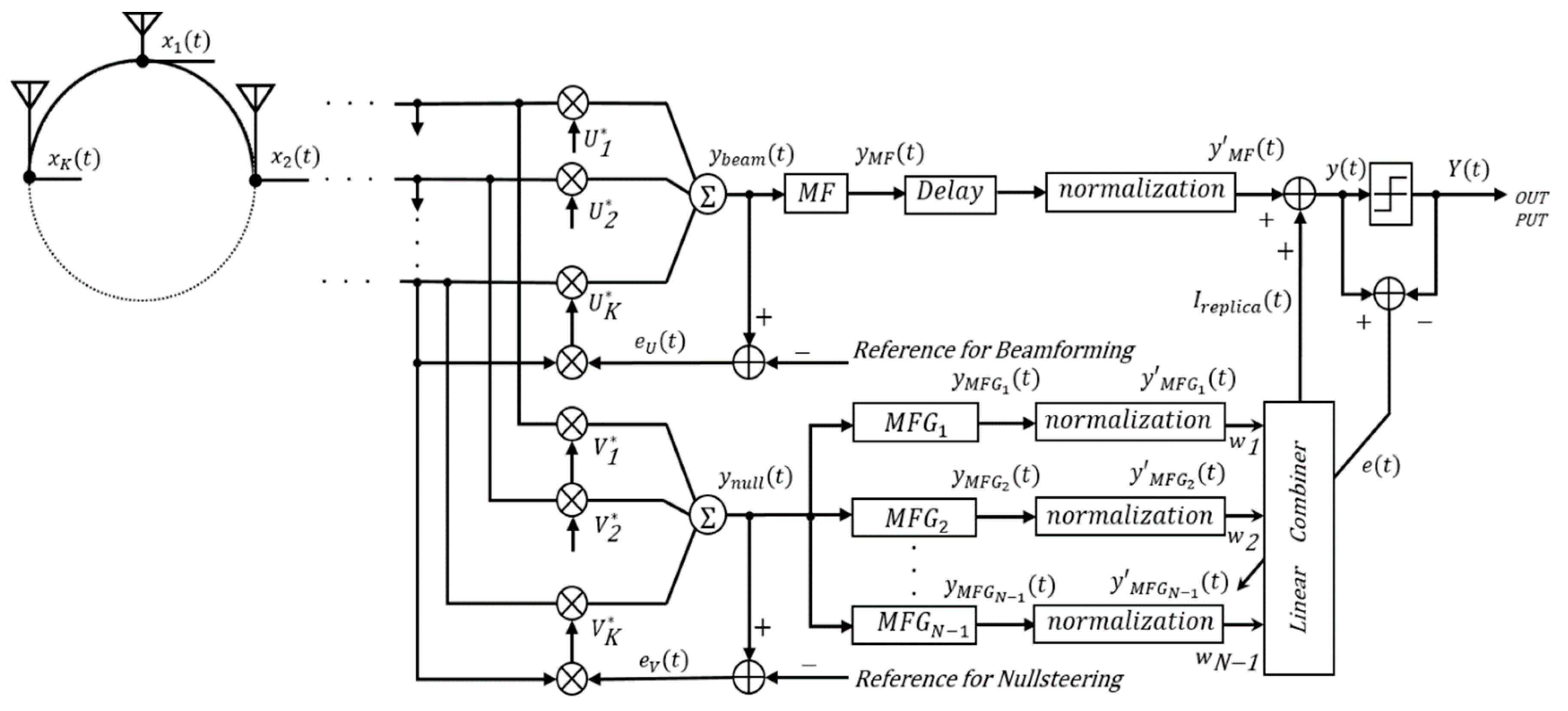
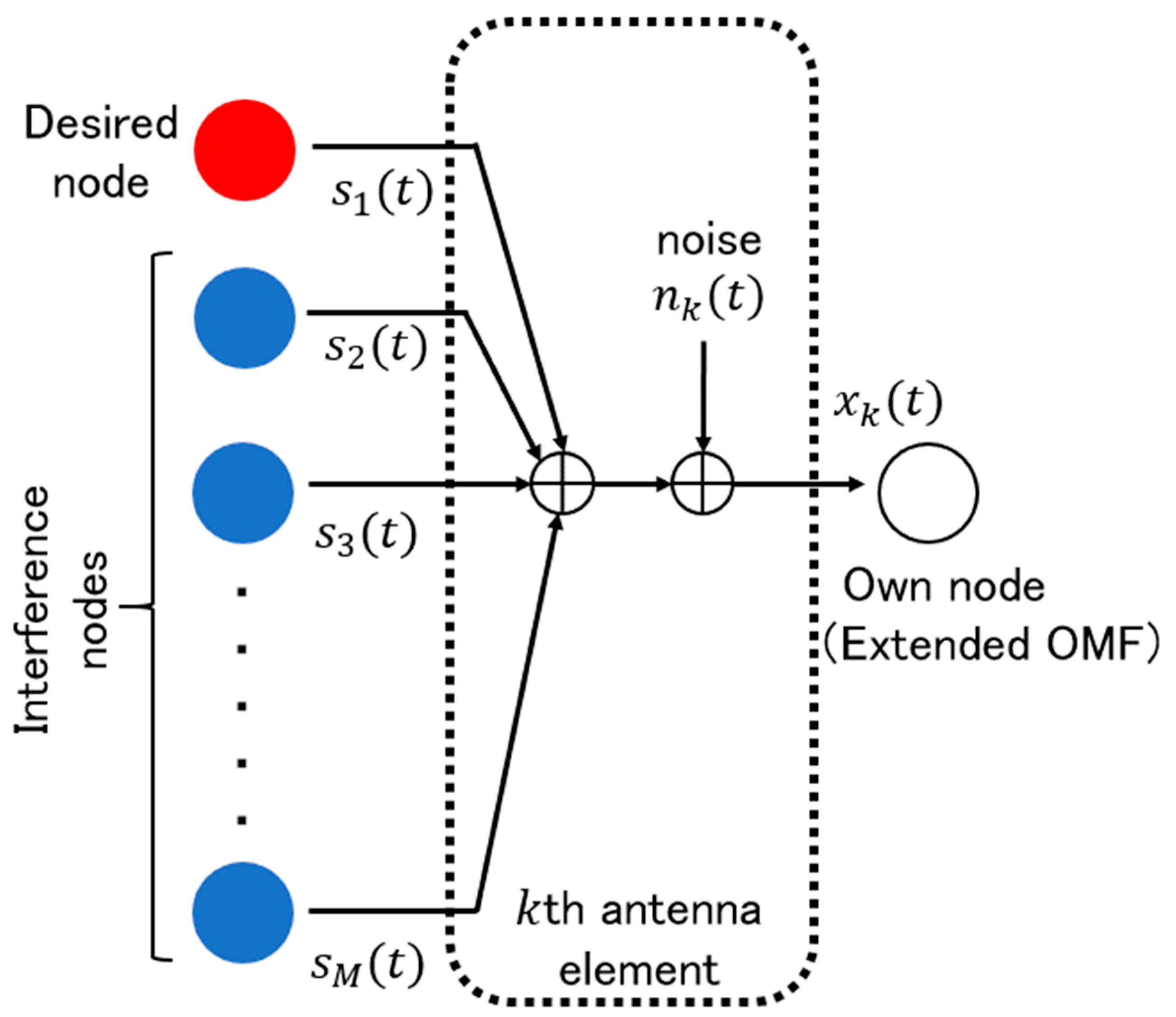
2.1. Structure of EOMF

Figure 1 and Figure 2 show a simplified structure of an EOMF and an assumed environment in this paper, respectively. $s_1\left(t\right)$, $s_2\left(t\right)$, …, $s_M\left(t\right)$ are the transmitted signals of each node. Binary phase shift keying (BPSK) is used for the primary modulation, and the direct-sequence spread-spectrum (DSSS) is used for secondary modulation. The transmitted signal of the m-th node, $s_m\left(t\right)$, is expressed as follows:

$$s_m\left(t\right)=\sqrt{2P_m}{d}_m\left(t\right){\mathit{c}}_m\left(t\right)\cos {\omega }_{c}t,$$

(1)

where, $d_m\left(t\right)$ ∈ {−1, 1} and $c_m\left(t\right)$ are the modulated data symbol for the BPSK and the spreading code of the mth node at time t, respectively [19,20]; and $P_m$ and ${\omega }_c$ are the transmitted signal power of the m-th node and the carrier frequency, respectively. In this paper, a baseband signal is used to simplify the discussion. In this case, the transmitted signal can be represented as follows:

$$s_m\left(t\right)=\sqrt{P_m}{d}_m\left(t\right){\mathit{c}}_m\left(t\right).$$

(2)

2.2. Circular Array Antenna

This paper assumes a circular array antenna [19,20,21,22]. The reason is that it can be applied not only to general mobile nodes but also to special applications such as a vehicle [20,22]. For example, refs. [20,22] assume a vehicle equipped with a circular array antenna as a VANET node. In a circular array antenna, K pieces of half-wave dipole antenna elements are arranged at half-wave intervals on a circle of radius R. Assuming that the input signal of the k-th (k = 1, 2, …, K) antenna element is $x_k\left(t\right)$, the input vector of the circular array antenna $\mathit{X}\left(t\right)$ = [$x_1\left(t\right)$, $x_2\left(t\right)$, …, $x_K\left(t\right)$]^T can be expressed as Equations (3)–(8).

$$\mathit{X}\left(t\right)=\mathit{A}\mathit{S}\left(t\right)+\mathit{\eta }\left(t\right)$$

(3)

$$\mathit{S}\left(\mathrm{t}\right)={\left[s_1\left(t\right),s_2\left(t\right),\dots ,s_M\left(t\right)\right]}^T$$

(4)

$$\mathit{A}=\left[\mathit{a}\left({\theta }_1\right),\mathit{a}\left({\theta }_2\right),\dots ,\mathit{a}\left({\theta }_M\right)\right]$$

(5)

$$\mathit{a}\left({\mathsf{\theta }}_m\right)=[ \exp (-j{\varphi }_1\left({\theta }_m\right), \exp (-j{\varphi }_2\left({\theta }_m\right),\dots ,\exp {\left(-j{\varphi }_K\left({\theta }_m\right)\right]}^T$$

(6)

$${\varphi }_k\left({\theta }_m\right)=\frac{2\pi }{\lambda }R\cos \left\{{\theta }_m-\frac{2\pi }{K}\left(k-1\right)\right\}$$

(7)

$$\mathit{\eta }\left(\mathrm{t}\right)={\left[n_1\left(t\right), n_2\left(t\right),\dots ,n_K\left(t\right)\right]}^T$$

(8)

where, $\mathit{a}\left({\mathsf{\theta }}_m\right)$ and ${\mathsf{\theta }}_m$ are the steering vector and the angle of arrival of the signal at the m-th node, respectively; $\lambda$ is the wavelength of the radio wave; $n_k\left(t\right)$ is the thermal noise of the k-th antenna element; and T is the transposition. In this research, it is assumed that the thermal noise is additive white Gaussian noise (AWGN) and there is no multipath fading to simplify the discussion. The output of the array antenna $y_{a\mathit{n}t}\left(t\right)$ can be expressed as following Equation (9):

$$y_{a\mathit{n}t}\left(t\right)=Re\left\{{\mathit{W}}^H\mathit{X}\left(t\right)\right\}= {\displaystyle \sum }_{k=1}^{K}Re\left\{W_k^{*}{x}_k\left(t\right)\right\}$$

(9)

where, Re {z} is the real part of the complex number z, $W_k$ is the weight of the k-th antenna element, and H and * are the Hermite transposition and complex conjugate, respectively.

In general, the optimal weight vector ${\mathit{W}}_{\mathrm{opt}}$ of an adaptive array antenna can be obtained by solving the Wiener–Hoff equation. This solution is called the Wiener solution and is represented as follows in Equation (10):

$${\mathit{W}}_{\mathrm{opt}}={\mathit{R}}_{xx}^{-1}{\mathit{r}}_{xr}$$

(10)

where, ${\mathit{R}}_{xx}$ is the correlation matrix of the input vector and is defined by the following Equation (11):

$${\mathit{R}}_{xx}\triangleq E\left[\mathit{X}\left(t\right)\mathit{X}{\left(t\right)}^H\right]$$

(11)

Then, $r_{xr}$ is a correlation vector between the reference signal r (t) and the input vector, and it is defined as follows in Equation (12):

$${\mathit{r}}_{xr}\triangleq E\left[\mathit{X}\left(t\right)r^{*}\left(t\right)\right]$$

(12)

Here, the reference signal r (t) is the transmission signal $s_1\left(t\right)$ of the first node (desired node). From the above Equations, the ${\mathit{R}}_{xx}$ and ${\mathit{r}}_{xr}$ of the circular array antenna that are used in the EOMF are derived as follows in Equations (13)–(16):

$${\mathit{R}}_{xx}={\displaystyle \sum }_{m=1}^M{P}_m\left[\begin{array}{c}\begin{array}{ccc}1& e^{-j\mathsf{\Phi }\left(1,2\right)}& \begin{array}{cc}\dots & e^{-j\mathsf{\Phi }\left(1,K\right)}\end{array}\end{array}\\ \begin{array}{ccc}{e}^{-j\mathsf{\Phi }\left(2,1\right)}& 1& \begin{array}{cc}\dots & e^{-j\mathsf{\Phi }\left(2,K\right)}\end{array}\end{array}\\ \begin{array}{c}\begin{array}{ccc}⋮& ⋮& \begin{array}{cc}\ddots & ⋮\end{array}\end{array}\\ \begin{array}{ccc}{e}^{-j\mathsf{\Phi }\left(K,1\right)}& e^{-j\mathsf{\Phi }\left(K,2\right)}& \begin{array}{cc}\dots & 1\end{array}\end{array}\end{array}\end{array}\right]+P_n{\mathit{I}}_K$$

(13)

$${\mathit{r}}_{xr}=P_1\left[\begin{array}{c}{e}^{-j{\varphi }_1\left({\theta }_1\right)}\\ e^{-j{\varphi }_2\left({\theta }_1\right)}\\ ⋮\\ e^{-j{\varphi }_K\left({\theta }_1\right)}\end{array}\right]$$

(14)

$$\mathsf{\Phi }\left(\iota ,\kappa \right)={\varphi }_{\iota }\left({\theta }_m\right)-{\varphi }_{\kappa }\left({\theta }_m\right)$$

(15)

$$P_n=E\left[{\left|n_k\left(t\right)\right|}^2\right]=2{\sigma }_{in}^2$$

(16)

where, ${\mathit{I}}_K$ is the K-th-order identity matrix. $P_1=E\left[{\left|s_1\left(t\right)\right|}^2\right]$ and $P_m=E\left[{\left|s_m\left(t\right)\right|}^2\right]$ ($m=2,3, \dots ,M$) are the input power of the desired signal and the interference signal, respectively. $P_n$ is the thermal noise power at each antenna element, and ${\sigma }_{in}^2$ is the noise variance.

2.3. OMF

The OMF consists of one matched filter (MF) with the same sequence as the desired node’s spreading sequence and N-1 matched filters (which is called the matched filter group: MFG) with a sequence that is orthogonal to the desired node’s spreading sequence [16,17,18,19,20]. N is the sequence length of the spreading sequence. A sequence that is orthogonal to the spreading sequence of the desired node is generated by Gram–Schmidt orthonormalization. A replica of the interference component that is included in the MF output is generated by weighting and adding the output of the MFG using a linear combiner (LC) controlled by an adaptive algorithm. The OMF can reduce the interference component of the MF output by using the replica of the interference component.

From (2), the received signal vector x that is obtained by sampling the spread signals that are transmitted from M nodes by N chips is expressed as follows in Equations (17) and (18):

$$\mathit{x}={\displaystyle \sum }_{m=1}^M\sqrt{P_m}{d}_m{\mathit{c}}_m+\mathit{n}$$

(17)

$${\mathit{c}}_m={\left[c_m\left(1\right), c_m\left(2\right),\dots ,c_m\left(N\right)\right]}^T$$

(18)

where, $\mathit{n}$ is the noise component for the N chips that are generated in the channel. Since the MF has the same sequence as the spreading sequence of the desired node, that is, c₁, the output of MF $x_{MF}$ is expressed by the following Equations (19) and (20):

$$x_{MF}={{\mathit{c}}_1}^T\mathit{x}=N\sqrt{P_1}{d}_1+{\displaystyle \sum }_{m=2}^M\sqrt{P_m}{d}_m{{\mathit{c}}_1}^T{\mathit{c}}_m+{{\mathit{c}}_1}^T\mathit{n}$$

(19)

$${{\mathit{c}}_1}^T{\mathit{c}}_1=N$$

(20)

In addition, ${\mathrm{MFG}}_i$ ($i=1,2,\dots ,N-1$) has a sequence ${\mathit{u}}_i=\left[u_i\left(1\right), u_i\left(2\right),\dots ,u_i\left(N\right)\right]$ that is orthogonal to ${\mathit{c}}_1$. Hence, the output of ${\mathrm{MFG}}_i$ $x_{MF{G}_i}$ is expressed as follows in Equations (21) and (22):

$$x_{MF{G}_i}={{\mathit{u}}_i}^T\mathit{x}={\displaystyle \sum }_{m=2}^M\sqrt{P_m}{d}_m{{\mathit{u}}_i}^T{\mathit{c}}_m+{{\mathit{u}}_i}^T\mathit{n}$$

(21)

$${{\mathit{u}}_i}^T{\mathit{c}}_1=0$$

(22)

Additionally, the LC’s weight vector w is defined as follows in Equation (23):

$$\mathit{w}\triangleq {\left[w_1, w_2,\dots ,w_{N-1}\right]}^T$$

(23)

The replica of the interference component included in $x_{MF}$ is generated by weighting and adding $x_{MF{G}_i}$ using the weight $w_i$. Therefore, the output of OMF $x_{OMF}$ is expressed as follows in Equation (24):

$$\begin{array}{cc}\hfill x_{OMF}& = x_{MF}+{\displaystyle \sum _{i=1}^{N-1}}{w}_i x_{MF{G}_i}\hfill \\ & =N\sqrt{P_1}{d}_1+{\displaystyle \sum _{m=2}^M}\sqrt{P_m}{d}_m{{\mathit{c}}_1}^T{\mathit{c}}_m+{{\mathit{c}}_1}^T\mathit{n}\hfill \\ & +{\displaystyle \sum _{i=1}^{N-1}}\left({\displaystyle \sum _{m=2}^M}\sqrt{P_m}{d}_m{{\mathit{u}}_i}^T{\mathit{c}}_m{w}_i+{{\mathit{u}}_i}^T\mathit{n}{w}_i\right)\hfill \end{array}$$

(24)

2.4. EOMF

As shown in Figure 1, the EOMF has a configuration in which an array antenna is incorporated at the start of the OMF [20]. If the desired signal to interference signal ratio (DIR) of the input signal is small, the OMF cannot sufficiently remove the interference signal. However, the DIR is improved since the input signal of the OMF in the EOMF is the output signal of the array antenna. However, the cancelled interference of the array antenna is insufficient when the arrival angle of the desired signal is close to that of the interference signal or when the degrees of freedom of the antenna are insufficient. However, since the array antenna output in the EOMF is input to the OMF, the residual interference components can be removed. Furthermore, the error convergence in the adaptive algorithm is improved by using the array antenna output that is beamformed on the desired signal as an input signal to the MF and the array antenna output null that is used as an input signal to the MFG in the EOMF.

The received signal vector of the MF, that is, the signal vector ${\mathit{y}}_{beam}$ that is beamformed for the desired signal, is expressed as follows from Equations (9) and (17), where the weight vector of the array antenna is defined as $\mathit{U}\triangleq {\left[U_1, U_2,\dots ,U_K\right]}^T$ in Equation (25):

$${\mathit{y}}_{beam}= {\displaystyle \sum }_{k=1}^{K}Re\left\{U_k^{*}{x}_k\right\}={\displaystyle \sum }_{k=1}^K\left({\displaystyle \sum }_{m=1}^M\sqrt{P_m}{d}_m{\mathit{c}}_{m}Re\left\{e^{-j{\varphi }_k\left({\theta }_m\right)}{U}_k^{*}\right\}+Re\left\{{\mathit{n}}_k{U}_k^{*}\right\}\right)$$

(25)

where, the correlation matrix and the correlation vector of U are the same as Equations (13) and (14), respectively. Likewise, the received signal vector of the MFG, that is, the signal vector ${\mathit{y}}_{null}$ used to null steer the desired signal, is expressed as follows, where the weight vector of the array antenna is defined as $\mathit{V}\triangleq {\left[V_1, V_2,\dots ,V_K\right]}^T$ in Equation (26):

$${\mathit{y}}_{null}= {\displaystyle \sum }_{k=1}^{K}Re\left\{V_k^{*}{\mathit{x}}_k\right\}={\displaystyle \sum }_{k=1}^K\left({\displaystyle \sum }_{m=1}^M\sqrt{P_m}{d}_m{\mathit{c}}_{m}Re\left\{e^{-j{\varphi }_k\left({\theta }_m\right)}{V}_k^{*}\right\}+Re\left\{{\mathit{n}}_k{V}_k^{*}\right\}\right)$$

(26)

However, the reference signal for null steering is the signal that is obtained by subtracting the reference signal for beamforming from the received signal [20]. Hence, the correlation matrix of V is the same as $\mathit{U}$, and the correlation vector of V, ${{\mathit{r}}_{xr}}^{\prime }$, is as follows in Equation (27):

$${{\mathit{r}}_{xr}}^{\prime }={\displaystyle \sum }_{m=2}^M{P}_m\left[\begin{array}{c}{e}^{-j{\varphi }_1\left({\theta }_m\right)}\\ e^{-j{\varphi }_2\left({\theta }_m\right)}\\ ⋮\\ e^{-j{\varphi }_K\left({\theta }_m\right)}\end{array}\right]$$

(27)

From (19) and (25), the output signal of the MF $y_{MF}$ is expressed by the following Equation (28):

$$\begin{array}{cc}\hfill y_{MF}& ={{\mathit{c}}_1}^T{\mathit{y}}_{beam}\hfill \\ & ={\displaystyle \sum _{k=1}^K}(N\sqrt{P_1}{d}_{1}Re\left\{e^{-j{\varphi }_k\left({\theta }_1\right)}{U}_k^{*}\right\}+{\displaystyle \sum _{m=2}^M}\sqrt{P_m}{d}_m{{\mathit{c}}_1}^T{\mathit{c}}_{m}Re\{e^{-j{\varphi }_k\left({\theta }_m\right)}{U}_k^{*}\}\hfill \\ & +{{\mathit{c}}_1}^{T}Re\left\{{\mathit{n}}_k{U}_k^{*}\right\})\hfill \end{array}$$

(28)

In (28), the first term, the second term, and the third term represent the desired signal component, the interference signal component and the noise component, respectively. Additionally, the output signal of the ${\mathrm{MFG}}_i$ $y_{{\mathrm{MFG}}_i}$ is expressed as following Equation (29) from Equations (21) and (26):

$$y_{{\mathrm{MFG}}_i}={\mathit{u}}_i{}^T{\mathit{y}}_{null}={\displaystyle \sum }_{k=1}^K\left({\displaystyle \sum }_{m=2}^M\sqrt{P_m}{d}_m{{\mathit{u}}_i}^T{\mathit{c}}_{m}Re\left\{e^{-j{\varphi }_k\left({\theta }_m\right)}{V}_k^{*}\right\}+{{\mathit{u}}_i}^{T}Re\left\{{\mathit{n}}_k{V}_k^{*}\right\}\right)$$

(29)

where, $y_{MF}$ and $y_{MF{G}_i}$ need to be normalized with respect to the desired signal component since the error signal that is used to update the weight vector of the LC is the difference between the output of the EOMF and its hard decision signal (+1 or −1). That is, the following Equation (30) needs to hold:

$$\left|\frac{{\sum }_{k=1}^{K}N\sqrt{P_1}{d}_{1}Re\left\{e^{-j{\varphi }_k\left({\theta }_1\right)}{U}_k^{*}\right\}}{{\sum }_{k=1}^{K}N\sqrt{P_1}Re\left\{e^{-j{\varphi }_k\left({\theta }_1\right)}{U}_k^{*}\right\}}\right|=\left|d_1\right|=1$$

(30)

In this research, (30) is assumed to hold for simplification. From the above, assuming that the normalized $y_{MF}$ and $y_{MF{G}_i}$ are ${y_{MF}}^{\prime }=\frac{y_{MF}}{\alpha }$ and ${y_{MF{G}_i}}^{\prime }=\frac{y_{MF{G}_i}}{\alpha }$, respectively, the output of the EOMF y is expressed as following Equation (31):

$$y={y_{MF}}^{\prime }+{\sum }_{i=1}^{N-1}{w}_i{y_{MF{G}_i}}^{\prime }=\frac{1}{\alpha }\left(y_{MF}+{\sum }_{i=1}^{N-1}{w}_i{y}_{MF{G}_i}\right) (\mathsf{\alpha }\ne 0)$$

(31)

3. Theoretical Analysis

3.1. Noise Free and Interference Channel

In this subsection, we derive the optimal solution for the noise free and interference channel. In this research, a weight vector that minimizes the mean squared error (MSE) that is expressed by the following Equation (32) is defined as the optimal solution:

$$E_{if}^2\triangleq {\left(y-\frac{1}{\alpha }{\displaystyle \sum }_{k=1}^{K}N\sqrt{P_1}{d}_{1}Re\left\{e^{-j{\varphi }_k\left({\theta }_1\right)}{U}_k^{*}\right\}\right)}^2$$

(32)

For a noise free channel, Equation (32) can be rewritten as follows in Equation (33):

$$\begin{array}{cc}\hfill E_{if}^2& =\frac{1}{{\alpha }^2}({\displaystyle \sum _{k=1}^K}{\displaystyle \sum _{m=2}^M}\sqrt{P_m}{d}_m{{\mathit{c}}_1}^T{\mathit{c}}_{m}Re\left\{e^{-j{\varphi }_k\left({\theta }_m\right)}{U}_k^{*}\right\}\hfill \\ & +{\displaystyle \sum _{i=1}^{N-1}}{w}_i{\displaystyle \sum _{k=1}^K}{\displaystyle \sum _{m=2}^M}\sqrt{P_m}{d}_m{\mathit{u}}_i{}^T{\mathit{c}}_{m}Re\left\{e^{-j{\varphi }_k\left({\theta }_m\right)}{V}_k^{*}\right\}{)}^2\hfill \end{array}$$

(33)

Therefore, the following Equation (34) is satisfied in the case of the optimal weight vector ${\mathit{w}}_{opt}$:

$${\displaystyle \sum }_{k=1}^K{{\mathit{c}}_1}^T{\mathit{c}}_{m}Re\left\{e^{-j{\varphi }_k\left({\theta }_m\right)}{U}_k^{*}\right\}=-{\displaystyle \sum }_{i=1}^{N-1}{\mathit{u}}_i{}^T{\displaystyle \sum }_{k=1}^K{\mathit{c}}_{m}Re\left\{e^{-j{\varphi }_k\left({\theta }_m\right)}{V}_k^{*}\right\}{w}_{opt,i}$$

(34)

The derivation of Equation (34) is shown in Appendix A. To derive ${\mathit{w}}_{opt}$, consider the following Equations (35)–(39):

$$\mathit{B}=-\mathit{C}{\mathit{w}}_{opt}$$

(35)

$${\mathit{w}}_{opt}=\{\begin{array}{c}-{\mathit{C}}^{-1}\mathit{B} \left(M=N\right)\\ -{\mathit{C}}^{+}\mathit{B} (M<N)\end{array}$$

(36)

$$\mathit{B}=\left[\begin{array}{c}\mathsf{{\rm Y}}\left(2\right)\\ ⋮\\ \mathsf{{\rm Y}}\left(M\right)\end{array}\right], \mathit{C}=\left[\begin{array}{ccc}{\mathit{u}}_1{}^T\mathsf{\Psi }\left(2\right)& \dots & {\mathit{u}}_{N-1}{}^T\mathsf{\Psi }\left(2\right)\\ ⋮& \ddots & ⋮\\ {\mathit{u}}_1{}^T\mathsf{\Psi }\left(M\right)& \dots & {\mathit{u}}_{N-1}{}^T\mathsf{\Psi }\left(M\right)\end{array}\right]$$

(37)

$$\mathsf{{\rm Y}}\left(m\right)={\displaystyle \sum }_{k=1}^K{{\mathit{c}}_1}^T{\mathit{c}}_{m}Re\left\{e^{-j{\varphi }_k\left({\theta }_m\right)}{U}_k^{*}\right\}$$

(38)

$$\mathsf{\Psi }\left(m\right)={\displaystyle \sum }_{k=1}^K{\mathit{c}}_{m}Re\left\{e^{-j{\varphi }_k\left({\theta }_m\right)}{V}_k^{*}\right\}$$

(39)

where, we can find only one ${\mathit{w}}_{opt}$ that satisfies $E_{if}^2$ = 0 if it is full rank as M = N. However, if $M<N$, there are multiple solutions that satisfy Equation (36). In this case, the adaptive algorithm allows $\mathit{w}$ to converge to the minimum Euclidean norm with ${\mathit{C}}^{+}$ as the Moore–Penrose pseudoinverse. As a result, M < N is necessary to completely eliminate the interference. Hence, an MF that exceeds the total number of nodes is required.

3.2. Noisy Interference Channel

In a noisy interference channel, the output of the EOMF when the interference is removed using ${\mathit{w}}_{opt}$ is expressed as following Equation (40) from Equations (28), (29), and (31):

$$y=\frac{1}{\alpha }\left\{{\displaystyle \sum }_{k=1}^K\left(N\sqrt{P_1}{d}_{1}Re\left\{e^{-j{\varphi }_k\left({\theta }_1\right)}{U}_k^{*}\right\}+{{\mathit{c}}_1}^{T}Re\left\{{\mathit{n}}_k{U}_k^{*}\right\}+{\displaystyle \sum }_{i=1}^{N-1}{w}_{opt,i}{\mathit{u}}_i{}^{T}Re\left\{{\mathit{n}}_k{V}_k^{*}\right\}\right)\right\}$$

(40)

Hence, the noise component increases by the number of MFs.

3.3. Residual Interference Due to Nonoptimal Weight Vector

If ${\mathit{w}}_{opt}$ in a noise free interference channel is used, the interference can be completely removed. However, if the weight vector has an error and it is not optimal, interference will remain. Ref. [19] considers an additional error $\mathit{\epsilon }$ and a multiplication error $\Delta$ as the errors in the weight vector to consider a non-optimal weight vector.

If the weight vector has $\mathit{\epsilon }$, it can be expressed as follows:

$${\mathit{w}}^{\prime }={\mathit{w}}_{opt}+\mathit{\epsilon }={\left[w_{opt,1}+{\epsilon }_1,w_{opt,2}+{\epsilon }_2, \dots ,w_{opt,N-1}+{\epsilon }_{N-1}\right]}^T$$

(41)

Using ${\mathit{w}}^{\prime }$ instead of ${\mathit{w}}_{opt}$, the output of the EOMF is as follows:

$$\begin{array}{c}y=\frac{1}{\alpha }\left\{{\displaystyle \sum _{k=1}^K}\right(N\sqrt{P_1}{d}_{1}Re\{e^{-j{\varphi }_k\left({\theta }_1\right)}{U}_k^{*}\}+{\mathit{c}}_1{}^{T}Re\{{\mathit{n}}_k{U}_k^{*}\}\hfill \\ +{\displaystyle \sum _{i=1}^{N-1}}({\displaystyle \sum _{m=2}^M}\sqrt{P_m}{d}_m{\mathit{u}}_i{}^T{\mathit{c}}_{m}Re\{e^{-j{\varphi }_k\left({\theta }_m\right)}{V}_k^{*}\}{\epsilon }_i+w_{opt,i}{{\mathit{u}}_i}^{T}Re\{{\mathit{n}}_k{V}_k^{*}\}\hfill \\ +{\epsilon }_i{{\mathit{u}}_i}^{T}Re\{{\mathit{n}}_k{V}_k^{*}\}\left)\right)\}\hfill \end{array}$$

(42)

In addition, y in a noise free environment is as follows:

$$y=\frac{1}{\alpha }\left\{{\displaystyle \sum }_{k=1}^K\left(N\sqrt{P_1}{d}_{1}Re\{e^{-j{\varphi }_k\left({\theta }_1\right)}{U}_k^{*}\}+{\displaystyle \sum }_{i=1}^{N-1}{\displaystyle \sum }_{m=2}^M\sqrt{P_m}{d}_m{\mathit{u}}_i{}^T{\mathit{c}}_{m}Re\{e^{-j{\varphi }_k\left({\theta }_m\right)}{V}_k^{*}\}{\epsilon }_i\right)\right\}$$

(43)

Hence, the interference is not completely removed due to $\mathit{\epsilon }$. In this case, the MSE of the output signal, $E_{sum}{}^2$, that is, the residual interference power, is expressed as follows:

$$\begin{array}{l}{E}_{s\mathit{u}m}{}^2=\frac{1}{{\alpha }^2}\left\{{\displaystyle \sum _{k=1}^K}\right({\mathit{c}}_1{}^{T}Re\left\{{\mathit{n}}_k{U}_k^{*}\right\}\hfill \\ +{\displaystyle \sum _{i=1}^{N-1}}({\displaystyle \sum _{m=2}^M}\sqrt{P_m}{d}_m{\mathit{u}}_i{}^T{\mathit{c}}_{m}Re\left\{e^{-j{\varphi }_k\left({\theta }_m\right)}{V}_k^{*}\right\}{\epsilon }_i+w_{opt,i}{\mathit{u}}_i{}^{T}Re\left\{{\mathit{n}}_k{V}_k^{*}\right\}\hfill \\ +{\epsilon }_i{\mathit{u}}_i{}^{T}Re\left\{{\mathit{n}}_k{V}_k^{*}\right\}\left)\right){\}}^2\hfill \end{array}$$

(44)

Next, if the weight vector has a scalar coefficient $\Delta$, it can be expressed as follows:

$${\mathit{w}}^{\prime }=\Delta {\mathit{w}}_{opt}={\mathit{w}}_{opt}+{\mathit{w}}_{opt}\left(\Delta -1\right)$$

(45)

That is, ${\mathit{w}}_{opt}\left(\Delta -1\right)$ can be regarded as $\mathit{\epsilon }$. By applying this to Equation (44), $E_{mul}{}^2$ is expressed as follows:

$$\begin{array}{c}{E}_{m\mathit{u}l}{}^2=\frac{1}{{\alpha }^2}\left\{{\displaystyle \sum _{k=1}^K}\right({\mathit{c}}_1{}^{T}Re\left\{{\mathit{n}}_k{U}_k^{*}\right\}\hfill \\ +{\displaystyle \sum _{i=1}^{N-1}}({\displaystyle \sum _{m=2}^M}\sqrt{P_m}{d}_m{\mathit{u}}_i{}^T{\mathit{c}}_{m}Re\{e^{-j{\varphi }_k\left({\theta }_m\right)}{V}_k^{*}\}{w}_{opt,i}(\Delta -1)\hfill \\ +w_{opt,i}{\mathit{u}}_i{}^{T}Re\{{\mathit{n}}_k{V}_k^{*}\}+w_{opt,i}(\Delta -1){\mathit{u}}_i{}^{T}Re\{\; stretchy="false"{\mathit{n}}_k{V}_k^{*}\}\left)\right){\}}^2\hfill \end{array}$$

(46)

3.4. Residual Noise Effect

Each component of the complex noise vector ${\mathit{n}}_k$ is normally distributed with mean $\mu$ and variance ${\sigma }_{in}^2$, and it is ergodic. For AWGN, $\mu$ = 0, and ${\sigma }_{in}^2$ represents the average power of the real and imaginary parts of the noise. That is, $P_n$ = 2${\sigma }_{in}^2$ for the total noise power, and the noise power on the real part of the signal is ${\sigma }_{in}^2$ = $P_n/2$. Here, since the norm of the spread sequence is $\parallel {\mathit{c}}_m\parallel {}^2=N$, the time average of the variance of the noise that has passed through the MF, ${\sigma }^2$, can be expressed as follows:

$${\sigma }^2=\frac{N}{{\alpha }^2}{\sigma }_{in}^2{\parallel \mathit{U}\parallel }^2$$

(47)

This is equal to the noise power that is contained in the de-spread signal of the array output. However, since the norm of ${\mathit{u}}_i$ that is found using the Gram–Schmidt orthonormalization method is $\parallel {\mathit{u}}_i\parallel =1$, the time average of the variance of the noise that is normalized by passing through the ${\mathrm{MFG}}_i$ is as follows:

$${\sigma }^2=\frac{1}{{\alpha }^2}{\sigma }_{in}^2{\parallel \mathit{V}\parallel }^2$$

(48)

Since the outputs of ${\mathrm{MFG}}_i$ are weighted by the LC and summed up, the residual noise that is contained in the output of EOMF, ${\sigma }_{sum}^2$, is expressed as follows:

$${\sigma }_{sum}^2=\frac{N}{{\alpha }^2}{\sigma }_{in}^2{\parallel \mathit{U}\parallel }^2+\frac{1}{{\alpha }^2}{\sigma }_{in}^2{\parallel \mathit{V}\parallel }^2{\parallel \mathit{w}\parallel }^2$$

(49)

Hence, in the EOMF, the noise is increased by the second term on the right side of Equation (49) and is emphasized, which increases the bit errors.

3.5. Optimal Weight Vector in an Interference and AWGN Channel

When the optimal weight vector ${\mathit{w}}_{opt}$ that is derived by Equation (36) is used, the interference component is completely removed from the EOMF output. However, as shown in Equation (49), the noise power is amplified and the MSE is increased. To suppress the effect, [19] considers the optimization of a scalar coefficient $\Delta \left(0\le \Delta \le 1\right)$ from Equation (46). Equation (46) shows that the noise component approaches zero and the interference component increases when $\Delta$ becomes close to zero; meanwhile, the interference component approaches zero and the noise component increases when $\Delta$ becomes close to one. Hence, they are expressed as following Equations (50) and (51):

$$\begin{array}{cc}\hfill \underset{\Delta \to 0}{\lim }{E}_{mul}{}^2\left(\Delta \right)=& \frac{1}{{\alpha }^2}\left\{{\displaystyle \sum _{k=1}^K}\right({\mathit{c}}_1{}^{T}Re\left\{{\mathit{n}}_k{U}_k^{*}\right\}\hfill \\ & -{\displaystyle \sum _{i=1}^{N-1}}{\displaystyle \sum }_{m=2}^M\sqrt{P_m}{d}_m{\mathit{u}}_i{}^T{\mathit{c}}_{m}Re\left\{e^{-j{\varphi }_k\left({\theta }_m\right)}{V}_k^{*}\right\}{w}_{opt,i}){\}}^2\hfill \end{array}$$

(50)

$$\underset{\Delta \to 1}{\lim }{E}_{mul}{}^2\left(\Delta \right)=\frac{1}{{\alpha }^2}{\left\{{\displaystyle \sum }_{k=1}^K\left({\mathit{c}}_1{}^{T}Re\left\{{\mathit{n}}_k{U}_k^{*}\right\}+{\displaystyle \sum }_{i=1}^{N-1}{w}_{opt,i}{\mathit{u}}_i{}^{T}Re\left\{{\mathit{n}}_k{V}_k^{*}\right\}\right)\right\}}^2$$

(51)

Hence, the optimal weight vector $\widehat{{\mathit{w}}_{opt}}$ that satisfies the minimum MSE (MMSE) that is calculated by the sum of the residual noise and residual interference is defined as following Equations (52) and (53):

$$\widehat{{\mathit{w}}_{opt}}=\arg \underset{0\le \Delta \le 1}{\min }\left(E_{mul}{}^2\left(\Delta \right)\right)={\Delta }_{opt}{\mathit{w}}_{opt}$$

(52)

$${\Delta }_{opt}\triangleq \arg \underset{0\le \Delta \le 1}{\min }\left(E_{mul}{}^2\left(\Delta \right)\right)$$

(53)

where, $E_{mul}{}^2\left(\Delta \right)$ is expressed by the following Equations:

$$\begin{array}{c}{E}_{mul}{}^2\left(\Delta \right)=\frac{N}{{\alpha }^2}{\sigma }_{in}^2{\parallel \mathit{U}\parallel }^2+\frac{{\Delta }^2}{{\alpha }^2}{\sigma }_{in}^2{\parallel \mathit{V}\parallel }^2\parallel {\mathit{w}}_{opt}\parallel {}^2+\frac{{\left(1-\Delta \right)}^2{G}_I{}^2}{{\alpha }^2}\beta =p{\Delta }^2+q\Delta +\gamma \hfill \\ = p{\left(\Delta +\frac{q}{2p}\right)}^2-\frac{q^2}{4p}+\gamma \hfill \end{array}$$

(54)

$$p={\left(\frac{1}{{\alpha }^2}{\sigma }_{i\mathit{n}}^2{\parallel \mathit{V}\parallel }^2\parallel {\mathit{w}}_{opt}\parallel {}^2+\frac{G_I{}^2}{{\alpha }^2}\beta \right)}^2$$

(55)

$$q=-2\frac{G_I{}^2}{{\alpha }^2}\beta$$

(56)

$$\gamma =\frac{N}{{\alpha }^2}{\sigma }_{in}^2{\parallel \mathit{U}\parallel }^2+\frac{G_I{}^2}{{\alpha }^2}\beta$$

(57)

$$\beta ={\displaystyle \sum }_{m=2}^M{\left({{\mathit{c}}_1}^T{\mathit{c}}_m\right)}^2\left\{{\left({\displaystyle \sum }_{k=1}^{K}Re\left\{e^{-j{\varphi }_k\left({\theta }_m\right)}\right\}Re\left\{U_k^{*}\right\}\right)}^2+{\left({\displaystyle \sum }_{k=1}^{K}Im\left\{e^{-j{\varphi }_k\left({\theta }_m\right)}\right\}Im\left\{U_k^{*}\right\}\right)}^2\right\}$$

(58)

where, $G_I$ is the interference power. Equation (54) is derived in detail in Appendix B. Equation (54) is obviously a quadratic Equation with respect to $\Delta$. Then, $E_{mul}{}^2\left(\Delta \right)$ is a downward convex function since $p\ge 0$. Hence, the ${\Delta }_{opt}$ for which $E_{mul}{}^2\left(\Delta \right)$ is minimized and the MMSE, $\min \left(E_{mul}{}^2\left(\Delta \right)\right)$, are derived as follows:

$${\Delta }_{opt}=-\frac{q}{2p}=\frac{G_I{}^2\beta }{{\sigma }_{i\mathit{n}}^2{\parallel \mathit{V}\parallel }^2\parallel {\mathit{w}}_{opt}\parallel {}^2+G_I{}^2\beta }$$

(59)

$$\min \left(E_{mul}{}^2\left(\Delta \right)\right)=-\frac{q^2}{4p}+\gamma =-\frac{{\left(G_I{}^2\beta /\alpha \right)}^2}{{\sigma }_{i\mathit{n}}^2{\parallel \mathit{V}\parallel }^2\parallel {\mathit{w}}_{opt}\parallel {}^2+G_I{}^2\beta }+\frac{N}{{\alpha }^2}{\sigma }_{in}^2{\parallel \mathit{U}\parallel }^2+\frac{G_I{}^2}{{\alpha }^2}\beta$$

(60)

From the above, the optimum weight vector $\widehat{{\mathit{w}}_{opt}}$ and the MMSE when using it can be derived.

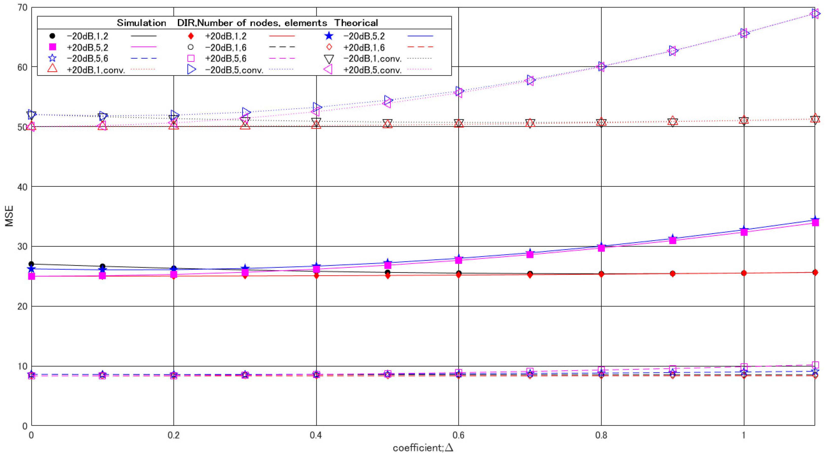
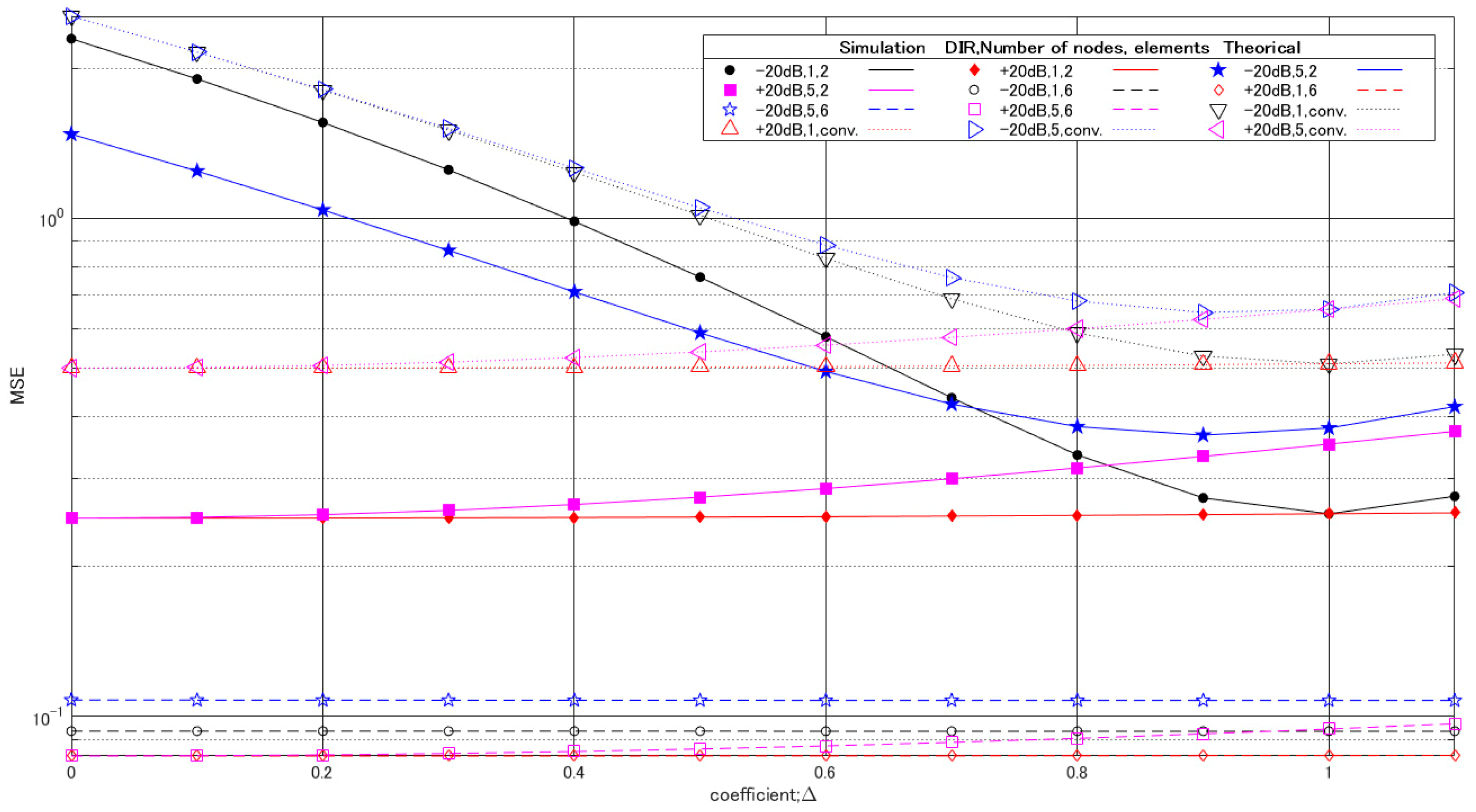
4. Numerical Results

This section compares the numerical results of the theoretical analysis and computer simulation. In addition, a comparison of the EOMF and the only conventional OMF case [16] is also performed.

Table 1. Computer simulation parameters.

Parameter	Detail
Channel model	AWGN
Modulation	BPSK and DSSS
Spreading sequence	Gold sequence
Spreading factor	7
Carrier frequency	760 [MHz]
Transmit power of desired node	1
Number of interference nodes	1 or 5
Number of antenna elements	2 or 6 (EOMF case) 1 (Only conventional OMF case [16])
Direction of arrival (desired node)	0 [degree]
Information data length	10,000 [bits]
Number of trials	10,000

AWGN: additive white Gaussian noise; BPSK: binary phase shift keying; DSSS: direct-sequence spread-spectrum; EOMF: extended orthogonal matched filter.

shows the simulation parameters. In the computer simulation, it is assumed that there is one desired node and one or five interference nodes, and the number of antenna elements of the EOMF is two or six. The reason for selecting these numbers of antenna elements is that each corresponds to the number of interferences. That is, the case of two antenna elements can deal with one interference, but not five interferences, while the case of six antenna elements can deal with both interference cases. For simplification, the transmission power of the desired node is normalized to one, and the arrival direction of the signal is zero degrees. The transmission powers of all the interference nodes are equal, and their signal arrival directions are equally divided by 360 degrees. Additionally, synchronous acquisition, synchronous tracking, and normalization are assumed to be ideal. The noise is assumed to be AWGN without considering multipath fading.

Figure 3 and Figure 4 compares the MSEs of the only conventional OMF case [16] and the EOMF that are obtained with the computer simulation and the theoretical analysis as a function of $\Delta$ in the case that $E_b/N_0=-20$ dB and $E_b/N_0=20$ dB, respectively. The derived theoretical curve agrees with the computer simulation results in each DIR, regardless of whether the number of interference nodes is one or five under both $E_b/N_0$ conditions. When the number of interfering nodes is the same, as $\Delta$ approaches one, each MSE approaches the same value under the two conditions with different DIRs. Compared to the MSE of the only OMF case, those of the EOMF are reduced. In particular, it is suppressed most under any condition when the number of antenna elements is six. In addition, the MSE of this case is almost constant under each $E_b/N_0$ condition.

Figure 5, Figure 6 and Figure 7 illustrate ${\Delta }_{opt}$ of the EOMF and the only OMF under various DIR and $E_b/N_0$ conditions. When there is one interfering node, ${\Delta }_{opt}$ approaches one if E_b/N₀ is high and the DIR is low while ${\Delta }_{opt}$ approaches zero if $E_b/N_0$ is low and the DIR is high. Additionally, in the case where the number of interfering nodes is five and the number of antenna elements is two, the Δ_opt increases as $E_b/N_0$ increases until $E_b/N_0$ = 5 dB, while Δ_opt decreases when $E_b/N_0$ > 5 dB and the DIR is higher than 7 dB. Furthermore, the ${\Delta }_{opt}$ in the case that the number of interference nodes is five is smaller than that in the case that the number of interference nodes is one.

Figure 8, Figure 9 and Figure 10 show the MMSE of the EOMF and the only OMF when the optimum weight vector $\widehat{{\mathit{w}}_{opt}}$ is used as the performance bound. As shown in these figures, the MMSE depends on both $E_b/N_0$ and the DIR. As an example, the MMSE of the EOMF with two antenna elements when $E_b/N_0$ = 20 dB is focused on. When the DIR $\ge$ 2 dB, the higher the DIR is, the smaller the MMSE. However, when the DIR < 2 dB, the lower the DIR is, the smaller the MMSE. This phenomenon is also seen in the other $E_b/N_0$ cases. Then, the EOMF with six antenna elements achieves smaller MMSE than other cases. Specifically, only it has the MMSE of about 0.001.

5. Discussion and Conclusions

This research theoretically derived the optimal weight vector of the EOMF $\widehat{{\mathit{w}}_{opt}}$ and the MMSE as its performance bound in the interference and AWGN channel environment. The comparison of the numerical results from the computer simulation and theoretical analysis showed the correctness of the theoretical analysis. The results also showed that $\widehat{{\mathit{w}}_{opt}}$ and the MMSE depended on both $E_b/N_0$ and the DIR.

Here, numerical results are also discussed. In the case that the number of interfering nodes was the same, each MSE approached the same value under the two conditions with different DIRs as $\Delta$ approaches one. The reason is that the interference component is removed as $\Delta$ approaches one and only the noise component remains according to Equation (46). Then, the MSE of the EOMF with six antenna elements was almost constant under each $E_b/N_0$ condition, because the interference signal could be sufficiently removed, and only the influence of noise appeared in those results. Additionally, the ${\Delta }_{opt}$ in the case of five interference nodes was smaller than that in the case of one interference node. This is because the amount of interference for each node is small, and the EOMF works to further remove noise from Equation (46) in the former case. Furthermore, there was a local maximum for each MMSE. This is due to the power inversion effect in which the stronger the interference component is, the better the interference suppression effect [21].

Future work includes deriving the theoretical bit error ratio (BER) and analysing the theoretical performance considering multipath fading.

References

1. Alameri, I.A. MANETS and Internet of Things: The Development of a Data Routing Algorithm. Eng. Technol. Appl. Sci. Res. 2018, 8, 2604–2608. [Google Scholar]
2. Reina, D.G.; Toral, S.L.; Barrero, F.; Bessis, N.; Asimakopoulou, E. The Role of Ad Hoc Networks in the Internet of Things: A Case Scenario for Smart Environments. In Internet of Things and Inter-Cooperative Computational Technologies for Collective Intelligence; Studies in Computational Intelligence; Bessis, N., Xhafa, F., Varvarigou, D., Hill, R., Li, M., Eds.; Springer: Berlin/Heidelberg, Germany, 2013; Volume 460, pp. 89–113. [Google Scholar]
3. Alnumay, W.; Ghosh, U.; Chatterjee, P.A. Trust-Based Predictive Model for Mobile Ad Hoc Network in Internet of Things. Sensors 2019, 19, 1467. [Google Scholar] [CrossRef] [PubMed]
4. Ye, Q.; Zhuang, W. Token-Based Adaptive MAC for a Two-Hop Internet-of-Things Enabled MANET. IEEE Internet Things J. 2017, 4, 1739–1753. [Google Scholar] [CrossRef]
5. Karlsson, J.; Dooley, L.S.; Pulkkis, G. Secure Routing for MANET Connected Internet of Things Systems. In Proceedings of the 2018 IEEE 6th International Conference on Future Internet of Things and Cloud (FiCloud), Barcelona, Spain, 6–8 August 2018. [Google Scholar]
6. Park, J.; Huang, K.; Cho, S.; Kim, D. Mobility-aware spatial interference cancellation for mobile ad hoc networks. In Proceedings of the 2010 International Conference on Information and Communication Technology Convergence (ICTC), Jeju, Korea, 17–19 November 2010. [Google Scholar]
7. Huang, K.; Andrews, J.G.; Guo, D.; Heath, R.W.; Berry, R.A. Spatial Interference Cancellation for Multiantenna Mobile Ad Hoc Networks. IEEE Trans. Inf. Theory 2012, 58, 1660–1676. [Google Scholar] [CrossRef] [Green Version]
8. Mordachev, V.; Loyka, S. On node density—Outage probability tradeoff in wireless networks. IEEE J. Sel. Areas Commun. 2009, 27, 1120–1131. [Google Scholar] [CrossRef]
9. Pinto, P.C.; Win, M.Z. Communication in a Poisson Field of Interferers--Part I: Interference Distribution and Error Probability. IEEE Trans. Wirel. Commun. 2010, 9, 2176–2186. [Google Scholar] [CrossRef]
10. Zanella, A.; Zorzi, M. Theoretical Analysis of the Capture Probability in Wireless Systems with Multiple Packet Reception Capabilities. IEEE Trans. Commun. 2012, 60, 1058–1071. [Google Scholar] [CrossRef]
11. Babich, F.; Comisso, M. Multi-Packet Communication in Heterogeneous Wireless Networks Adopting Spatial Reuse: Capture Analysis. IEEE Trans. Wirel. Commun. 2013, 12, 5346–5359. [Google Scholar] [CrossRef]
12. Kim, C.; Cho, Y. Performance of a wireless MC-CDMA system with an antenna array in a fading channel: Reverse link. IEEE Trans. Commun. 2000, 48, 1257–1261. [Google Scholar]
13. Sanada, Y.; Padilla, M.; Araki, K. Performance of adaptive array antenna with multicarrier DS/CDMA in a mobile fading environment. IEICE Trans. Commun. 1998, E81-B, 1392–1399. [Google Scholar]
14. Ahn, C.J.; Sasase, I. Code Orthogonalizing Filter Based Adaptive Array Antenna Using Common Correlation Matrix of Time Domain Signals for Multicarrier DS/CDMA Systems. IEICE Trans. Fundam. Electron. Commun. Comput. Sci. 2002, E85A, 1604–1611. [Google Scholar]
15. Sakakibara, S.; Ohno, K.; Itami, M. Performance evaluation of DS-CDMA IVC scheme and CSMA/OFDM IVC scheme. In Proceedings of the 2013 13th International Conference on ITS Telecommunications (ITST), Tampere, Finland, 5–7 November 2013. [Google Scholar]
16. Hachisuka, M. Interference Cancellation Using Layered Structure of Orthogonal Matched Filter for Inter-Vehicle Communication and Ranging. Master’s Thesis, Yokohama National University, Yokohama, Japan, 2014. [Google Scholar]
17. Kobayashi, T.; Sugimoto, C.; Kohno, R. Interference Cancellation for Intra and Inter UWB Systems Using Modified Hermite Polynomials Based Orthogonal Matched Filter. IEICE Trans. Commun. 2016, E99.B, 569–577. [Google Scholar] [CrossRef]
18. Kobayashi, T.; Suzuki, M.; Sugimoto, C.; Kohno, R. Space Temporal Interference Cancellation Using TDL Array Antenna and Waveform Based OMF for IR-UWB Systems. ICT Express 2015, 1, 71–75. [Google Scholar] [CrossRef]
19. Kobayashi, T.; Sugimoto, C.; Kohno, R. Theoretical analysis of interference canceler using modified hermite polynomials based orthogonal matched filter for IR-UWB systems in AWGN and interference channel. In Proceedings of the 2017 20th International Symposium on Wireless Personal Multimedia Communications (WPMC), Bali, Indonesia, 17–20 December 2017. [Google Scholar]
20. Suzuki, M. Extended Orthogonal Matched Filter into Space and Time Domains for Cancelling Interference in Inter-Vehicle Communication and Radar. Master’s Thesis, Yokohama National University, Yokohama, Japan, 2016. [Google Scholar]
21. Kikuma, N. Adaptive Signal Processing with Array Antenna; Science and Technology Publishing Company Inc.: Tokyo, Japan, 1998. (In Japanese) [Google Scholar]
22. Masui, K.; Itami, M. Interference reduction in DS/SS inter-vehicle communication using circular array antenna. In Proceedings of the 2008 IEEE International Conference on Vehicular Electronics and Safety, Columbus, OH, USA, 22–24 September 2008. [Google Scholar]
Figure 1. Simplified structure of the extended orthogonal matched filter (EOMF).
Jsan 08 00048 g001
Figure 2. System model.
Jsan 08 00048 g002
Figure 3. Mean squared error (MSE) as a function of Δ . The dots are the results of the computer simulation and lines are the theoretical curves under interference signal ratio (DIR) = ± 20 dB, the number of interfering nodes is one or five, the number of antenna elements is two or six and E b / N 0 = 20 dB.
Jsan 08 00048 g003
Figure 4. MSE as a function of Δ . The dots are the results of the computer simulation and lines are the theoretical curves under DIR = ± 20 dB, the number of interfering nodes is one or five, the number of antenna elements two or six and Eb/N0 = 20 dB.
Jsan 08 00048 g004
Figure 5. Δ o p t of the EOMF with two antenna elements under various DIR and Eb/N0 conditions. (a) The number of interference nodes is one. (b) The number of interference nodes is five.
Jsan 08 00048 g005
Figure 6. Δ o p t of the EOMF with six antenna elements under various DIR and Eb/N0 conditions. (a) The number of interference nodes is one. (b) The number of interference nodes is five.
Jsan 08 00048 g006
Figure 7. Δ o p t of the only OMF under various DIR and Eb/N0 conditions. (a) The number of interference nodes is one. (b) The number of interference nodes is five.
Jsan 08 00048 g007
Figure 8. The minimum MSE (MMSE) of the EOMF with two antenna elements under various DIR and E b / N 0 conditions. (a) The number of interference nodes is one. (b) The number of interference nodes is five.
Jsan 08 00048 g008
Figure 9. The MMSE of the EOMF with six antenna elements under various DIR and E b / N 0 conditions. (a) The number of interference nodes is one. (b) The number of interference nodes is five.
Jsan 08 00048 g009
Figure 10. The MMSE of the only OMF under various DIR and E b / N 0 conditions. (a) The number of interference nodes is one. (b) The number of interference nodes is five.
Jsan 08 00048 g010