1. Introduction
The internet of things is promising to revolutionize almost all aspects of our life. From the way that we experience and communicate with our environment to the way that we manufacture our products and conduct business. This revolution is heavily based on the deployment of a myriad of smart things that sense, act, and communicate with the users and among themselves in order to provide advanced services. One of the first areas that are starting to experience this revolution is “smart homes”. According to a definition by the United Kingdom Department of Trade and Industry “A smart home is a dwelling incorporating a communications network that connects the key electrical appliances and services, and allows them to be remotely controlled, monitored or accessed.” An interpretation of this could be that a smart home is a house that includes multiple sense and actuate systems that allows to the users fully control and monitor functions such as lightning, heating and cooling, security and access, etc. From the aforementioned definition of the common smart home scenarios, it is clear that a smart home has rigid networking requirements for the connectivity of the smart things with the actuators and with the operators of the system; which are in the near zero latency range (e.g., if you need to open a garage door or a valve in a heating system the acceptable latency for the user is at the sub-second range). We have faced similar strict requirements during our deployment for the data collection and processing. This time the main issue was not the latency but the quality of the data. The quality of the data is affecting the results of the analytics and therefore it is fundamental for the precision of the system to deal with all root causes during collection, transfer, processing, and analysis of the data beforehand.
The remainder of the paper is structured as follows.
Section 2 provides an overview of the PeerEnergyCloud project and discusses the overall system architecture.
Section 3 describes the data quality challenges that we faced during the deployment with focus on the main analytical components of our system.
Section 4 presents the detailed analysis of the data quality issues we faced when piloting the system together with technical details of the key components in our test bed and the mechanisms for addressing the encountered challenges.
Section 5 discuss similar projects and, finally, we conclude the paper and discuss future work in
Section 6.
2. Project Background
In this paper, we present analysis of data that we acquired throughout a three year pilot with smart home technology. The pilot was conducted as part of the PeerEnergyCloud project [
1], which funded by the German federal ministry of technology. We describe the project background and the setting for our data collection in this section.
The PeerEnergyCloud was conducted between 2011 and of 2014 by a consortium of academic institutions and industry. The goal was to coordinate energy consumption within local neighborhoods to better utilize locally available renewable energy. Specifically, it aimed at finding a means to influence consumption behavior, so that energy from privately owned solar panels is consumed within the immediate neighborhood. Such an adaption of consumption behavior is of high interest for electrical grid operators, because it improves grid stability and saves investments in grid infrastructure [
2]. In addition, the project explored ways of how grid operators can provide additional services to the home owners on top of the piloted infrastructure. The PeerEnergyCloud project addressed the development of analytics technologies that enable a smarter use of energy. Specific use cases are detailed in
Section 3. All scenarios are driven by a deeper understanding of energy consumption on the level of individual households. The pilot in PeerEnergyCloud enabled this work though a cloud based infrastructure for data collection, processing, and service provisioning.
A central aspect of the project was the piloting of smart home sensor systems and applications. The smart home systems are the backbone of the PeerEnergyCloud project approach. Smart home solutions are the enabling technology that allows home owners to better understand and manage their energy consumption. As such, the technology provides the entry point for applications that help to optimize the consumption behavior and to deliver additional services. The pilot in the PeerEnergyCloud project allows deep insights into the operations of smart home system under real world conditions. Throughout the project, we collected data from smart home systems over a period of up to three years. This enables a long term analysis of the properties of smart home data and provides the basis for the results in this paper.
2.1. System Architecture
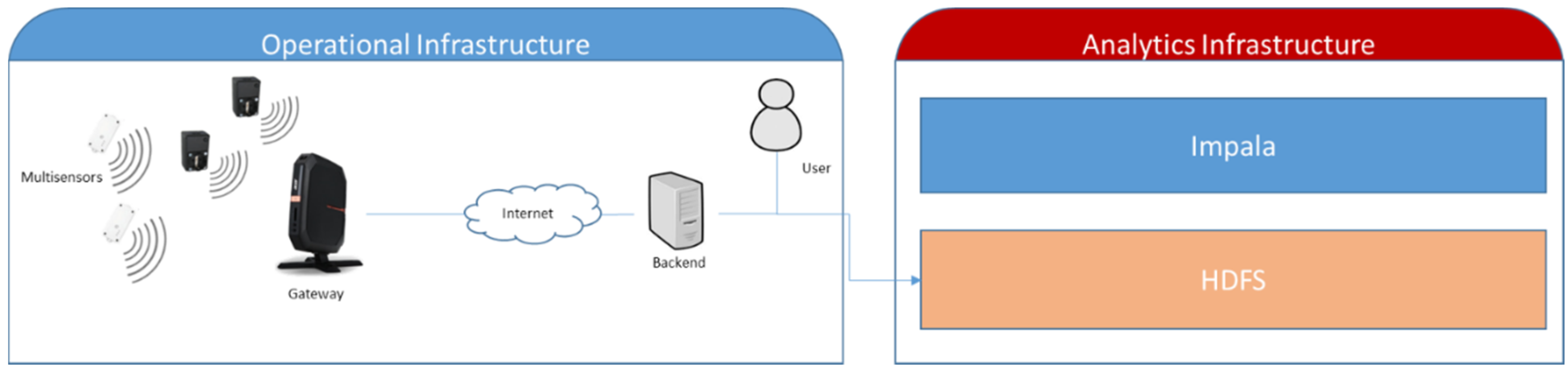
As depicted in
Figure 1, our system consists of two parts: the operational infrastructure that collects data from households and an analytics infrastructure that we used for analyzing the collected data. Data is transferred into the analytics infrastructure via batch process that export the data from PostgreSQL into Hadoop Distributed File System (HDFS) as Comma Separated Values (CSV) files. We used Impala to convert the CSV data to the parquet file format.
PostgreSQL was chosen because it provided an easy way of storing and querying the data using the SQL query language. However, we experienced that PostgreSQL is insufficient for performing
ad hoc queries as needed for the results presented in this paper. Running Impala on top of HDFS filled this gap. We also used additional infrastructures such as Hadoop’s Map Reduce, Storm, and the complex event processing engine Esper [
3].
The technological components of the system (of interest for this work) are the following:
Smart plugs with remote control, containing a high-precision energy meter to measure parameters like voltage, current, frequency, power, and electrical consumption (KWh). Measured data are sent via wireless connection (ZigBee [
4]) to the Home Gateway. Smart plugs contain a relay to switch on/off the devices remotely and consume only a few mA for all the operations carried out.
Multi-sensors able to acquire various ambient parameters like brightness, temperature, humidity, motion detection. Also in this case, measured data are sent via wireless connection (ZigBee) to the Home Gateway.
Home Gateway which collects all measured data, stores them in a local cache and sends them using a secure connection to a remote Backend. The gateway provides at least two interfaces: one wireless interface (ZigBee) able to connect to the smart plugs; one Ethernet/Wi-Fi interface to the home modem/router to have Internet access.
The analytics infrastructure consists of a small four-node Cloudera cluster. For the quality analysis presented in this paper we were only using the Impala service using YARN as a resource manager.
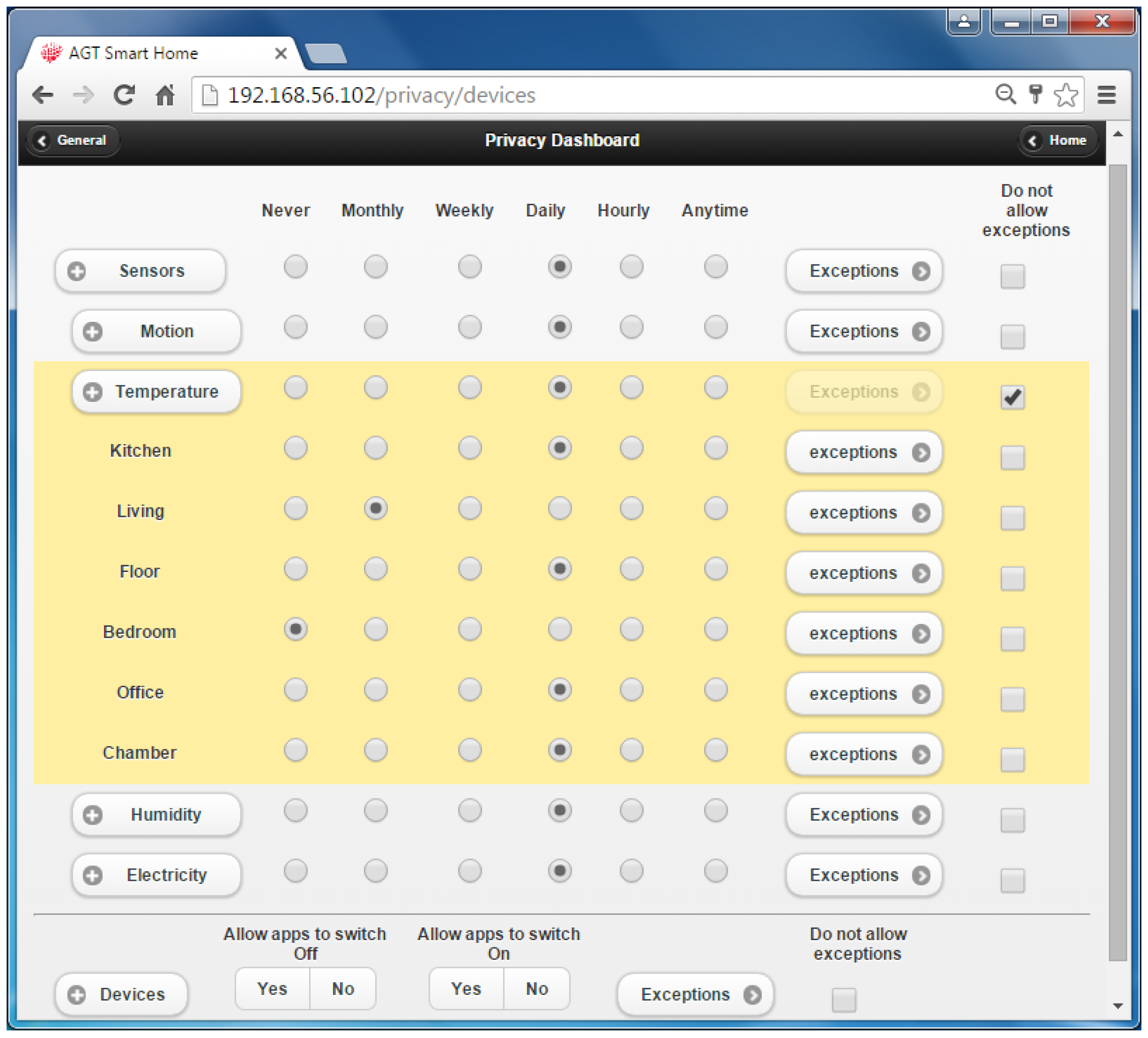
The smart metering ecosystem may facilitate a multitude of applications and value added services (VAS). Security and privacy are a major concern in this context as these applications and services directly affect users′ everyday life and may collect a substantial amount of sensitive data. In order to enable these services new security and privacy solutions are required. The user needs simple-to-use mechanisms that provide a transparent view on all data that is collected and processed within such an ecosystem. The user should be in perfect control of which data is collected, how it is processed and which data is exchanged with which third parties. The PEC Privacy Dashboard is one of the components developed for the PEC project designed to define and control access to sensors. The user interacts with this component dashboard to review current access control rules and to modify as well as add rules (see
Figure 2).
The user input from the privacy dashboard is transformed into statements in a given policy language. In order to make our approach as open as possible, XACML is used as the policy decision language, as its expressiveness allows full coverage of all necessary aspects for our application scenarios. These policy statements are then used to evaluate access requests from various applications. More details can be found in [
5].
2.2. Sensor Deployment
We provided some volunteers with smart home packages that have been installed on their premises. A package consisted of a set of sensors and a gateway to enable communication with a cloud infrastructure. In addition, volunteers had access to some cloud-based smart home applications. The volunteers conducted the installations on their own account and they were free in choosing how and where to install the sensors. Some of the initial installations were done under supervision from members of the research team and some completely unsupervised. From this point on, we continuously collected the data without any supervision of the deployment, in some cases for more than three years.
During the installation we faced some connectivity issues related to the connection of ZigBee devices to the gateway. The ZigBee connectivity heavily depended on the conditions within the various households. That is, the material of the wall and the distance between sensors (i.e., number of stories) had a strong impact on the connection quality. We managed to support deployment in large households by leveraging the multi-hop capabilities of the ZigBee protocol and by carefully selecting deployment positions (i.e., plugs in stairways between stories).
3. Data Quality Challenges in Smart Home Applications
Data quality is an important factor in any data driven application but the particular requirements vary between the particularities of the targeted use cases. Smart home technology is an enabler for a broad range of applications for a variety of stakeholders. The PeerEnergyCloud covered use cases that address the utilization of smart home technology for private users within the home as well as for optimizing the operations of utilities. The different applications are sensitive to different data quality aspects and to varying degrees. This section discusses the impact of data quality along sample use cases from the PeerEnergyCloud project. In particular, we address the data quality aspects of (a) data accuracy; (b) completeness; and (c) delay. Here, data accuracy refers to the correctness of captured sensor measurements. Completeness refers to the presence of absence of gaps in the sensor stream, and delay refers to the time gap between a change in the physical world and the reflection of this change in the software system. We discuss the significance of each aspect along the sample applications below and provide corresponding technical analysis throughout the paper. Specifically, we discuss (1) a real-time dashboard; (2) long-term consumption analysis; and (3) short-term consumption prediction.
3.1. Real-Time Dashboard
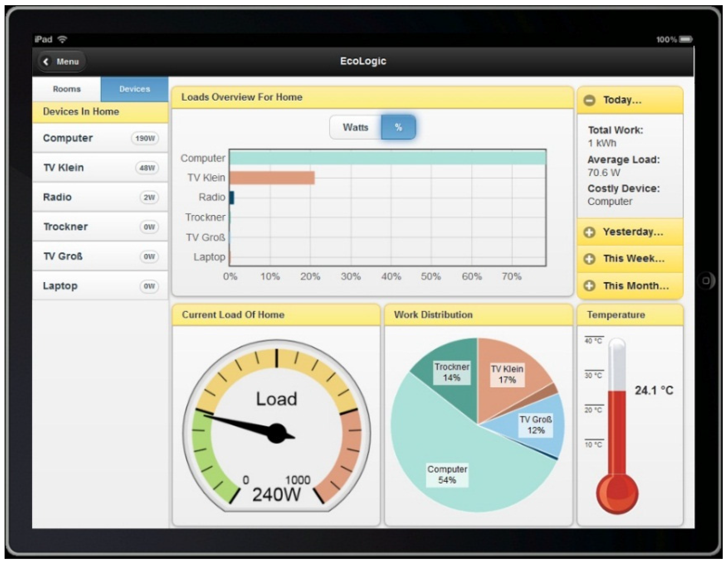
Trial participants of the PeerEnergyCloud project were provided with a set of web-based applications to analyze their consumption data. One of the key applications in this set is a real-time dashboard. Real-time in this application means, that users should get an instant feedback about changing their consumption. This is, when the user switches a device, the observed values must change quick enough for the user to relate the consumption change to his or her switching action.
Figure 3 shows a screenshot of the application. The dashboard provides live statistics of device specific energy consumption. Available visualizations are the current values as number as well as line charts that get continuously updated. The application furthermore enabled switching of devices via the web-interface.
Throughout the PeerEnergyCloud project this application was one of the main ways how users interacted with the system. Displaying correct data is vital for the perceived usefulness and the trust in the technical solution. In particular, values that are implausible can easily be spotted by users and lead to negative perceptions. Note that this aspect does not only relate to the correctness of sensor measurements. The completeness and timeliness of arrival is even more important. When users switch a device on, they expect the displayed load curves to go up immediately. However, missing or delayed values may cause a misalignment between the expected and the displayed data. Incorrect reflection of loads in the real-time dashboard is very prominently perceived by the users (e.g., I just switched the lamp is on but shows still a flat consumption line at zero). This makes dealing with gaps and delays in the data particularly challenging for such types of applications.
3.2. Long-Term Consumption Analysis
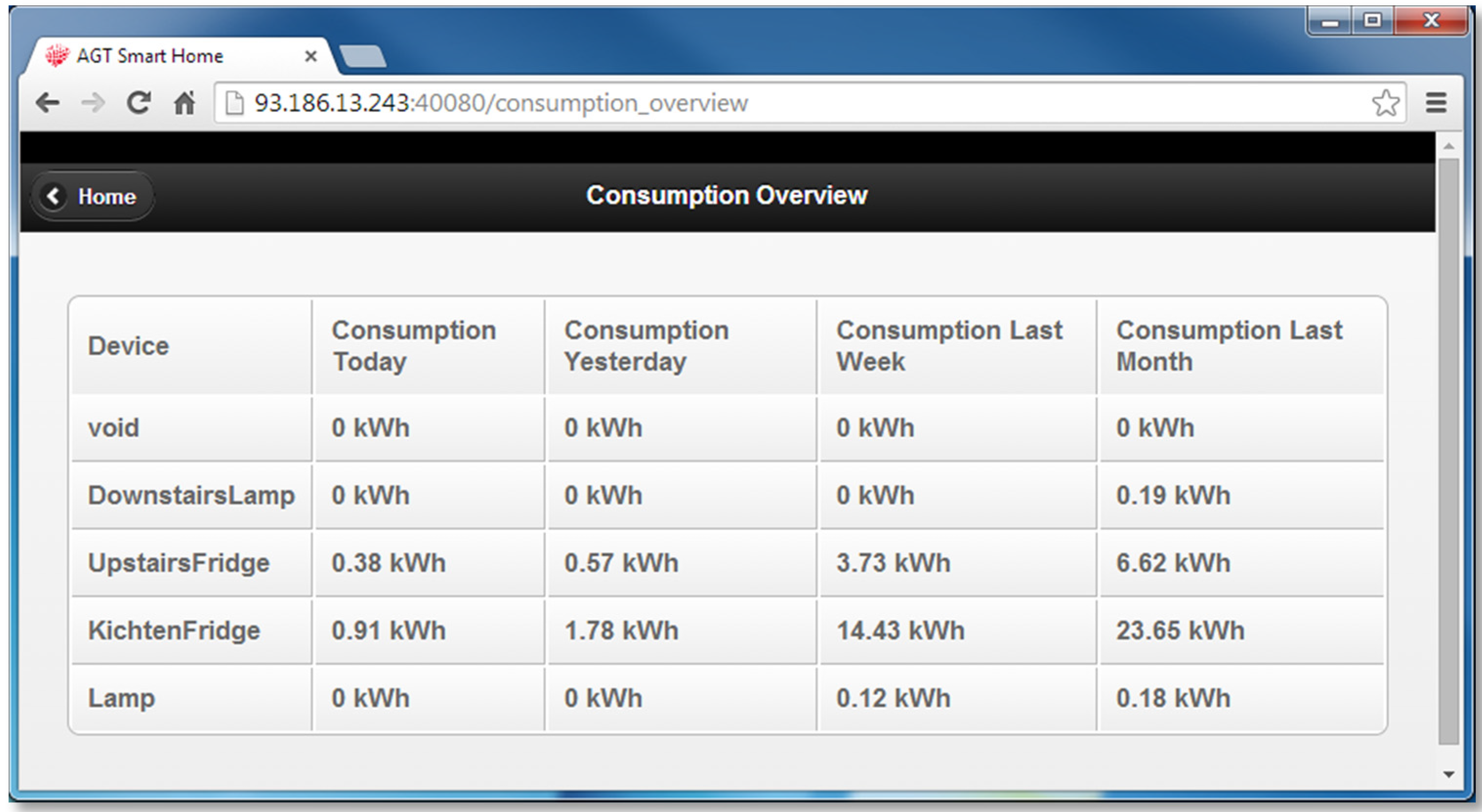
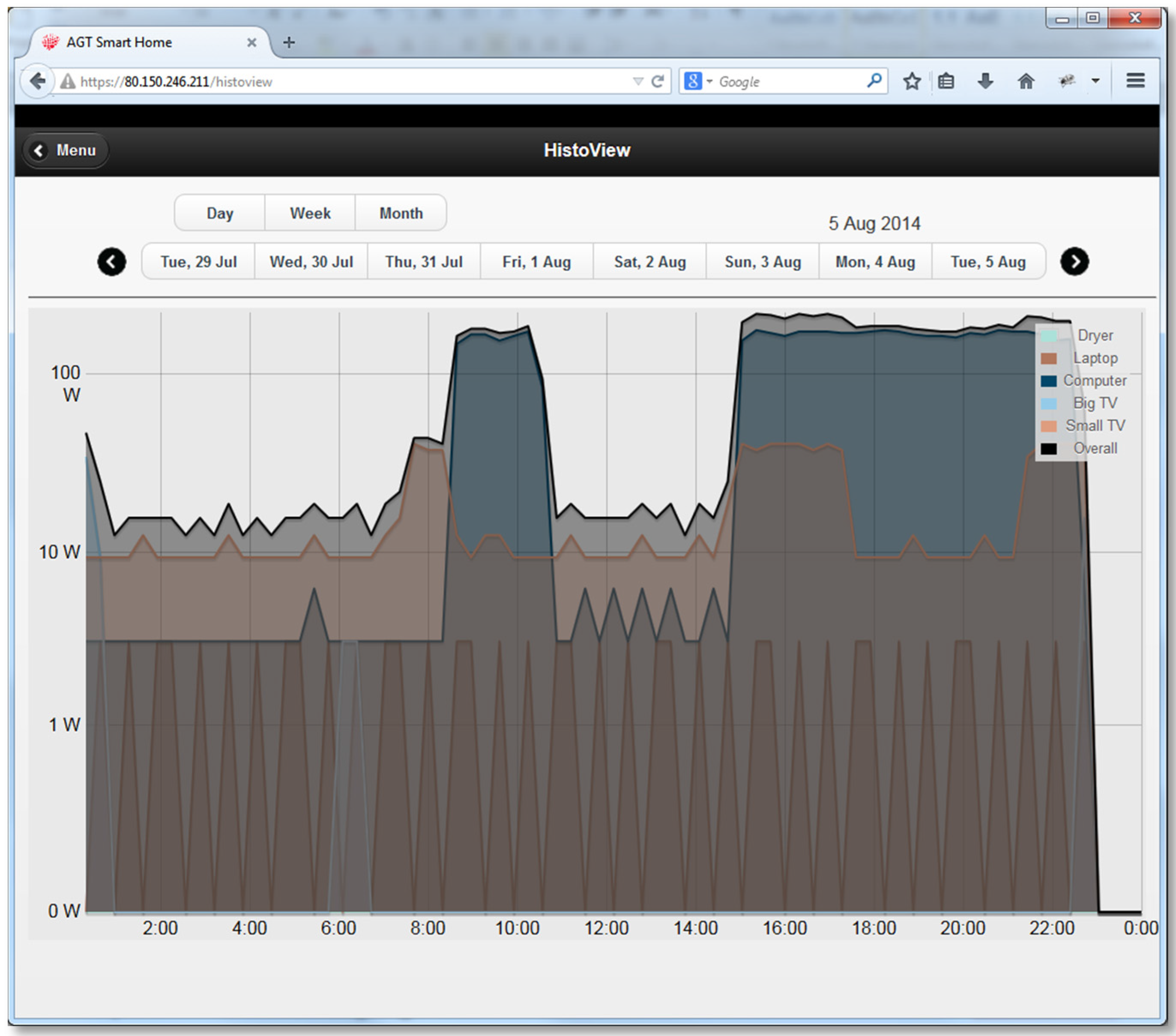
Part of the application portfolio within the PeerEnergyCloud project were applications that provide a long term analysis of device specific energy consumption. That is, consumption is displayed aggregated over days, week or month.
Figure 4 and
Figure 5 show sample screenshots of such applications from the pilot. The aggregated long term analysis was a key feature for many pilot participants. This is because it allows a better understanding how much a particular devices contribute to the overall consumption and how energy efficient they are overall. For instance, several users were keen to monitor the consumption of their washing machine to understand the impact of using older machines compared to modern and more energy efficient solutions.
Data quality for long term analysis must be sufficient to yield reasonably accurate results. Compared to real-time analysis, it is less critical if some measurements as missing, as long as the long term aggregate is not significantly impacted. Also, the applications do not display real-time updates and hence users do not directly perceive small gaps in the data stream. Thus, delays in measurements play a minor role for this type of application. However, throughout the pilot we encountered data quality issues that got to the users attention with negative effects on the perceived usefulness and trust in the system. The relevant data quality aspects are related to data accuracy and completeness. Erroneous measurements can in extreme cases lead to considerable distortion of the aggregate values and noticeably implausible results. Also, long gaps can cause apparent deviations from the actual and displayed consumption. For instance, a user may remember to have briefly watched TV yesterday but—in case of a longer measurement gap—may see zero consumption for the TV on that day. Thus, while being less time critical, scrutinizing data for display is required and the quality of the input streams has a significant impact on the applications.
3.3. Short-Term Consumption Prediction
A key challenge for grid operators is balancing out production and consumption at any time. Growing numbers of solar panels on private homes in Germany introduce additional complexity to this challenge. For efficiency reasons, it is desirable to balance out the production and consumption locally in the grid and avoid long distance energy transmission. One goal of the PeerEnergyCloud project was to investigate means for improving local balancing by proactively influencing energy consumption in households. Proactive steering however, requires household specific prediction of the consumption at least a few minutes ahead [
6].
Throughout the project, we investigated prediction mechanisms that apply household specific prediction models on the real-time streams of consumption data. Our experiments show that high resolution and device specific measurements enable improvements in the short-term prediction accuracy. Yet, data quality issues can impact the prediction. One aspect is that faulty input data causes prediction errors. Another aspect, is that missing data reduces the prediction accuracy as well. We have shown in experiments, that high temporal resolutions in measurements can positively impact the prediction accuracy [
5]. Thus, the data accuracy is major concern for short-term consumption prediction. The aspect of delay however is comparatively less relevant. This is because the temporal scope for predictions is in the order of at least several minutes. Thus, compared in dashboards for real-time consumption monitoring, delays of a few seconds have less impact on an application level.
4. Analysis of Data Quality
This section presents the results of our analysis of data quality. We first provide an overview of the overall characteristics of the captured data and the observed anomalies. Subsequently, we report on findings regarding the arrival rates of sensors messages and the downtimes of infrastructure components.
4.1. Overview of Data Characteristics
Overall, the data quality of six households has been analyzed. Each household contained six or seven smart plugs and all but one contained three or four multi-sensor devices.
Table 1 details the distribution of sensing devices and the total number of measurements. While most households provided between 520 and 650 Mio measurements, Houses 4 and 6 only delivered a fraction of the measurements. This is due to the fact that House 6 was configured with a lower sampling rate and only reported one sample per minute as compared to a sample of every two seconds at the other houses. Each smart plug includes six sensors and each multi-sensor device contains five sensors.
Table 1 and
Table 2 give an overview of the captured data types and total number of measurements.
Overall, we examined the data quality of over 2.5 billion measurements that were stored in a single, de-normalized, partitioned Impala table backed by parquet files using the default snappy compression. Several additional, auxiliary tables were created supporting the analysis. The files were stored on HDFS using our default replication factor of three. The net storage,
i.e., not counting the replicated blocks, of the compressed parquet files amounts to approximately 17 GB of data. As comparison the uncompressed net storage of the same data on HDFS amounts to approximately 287 GB.
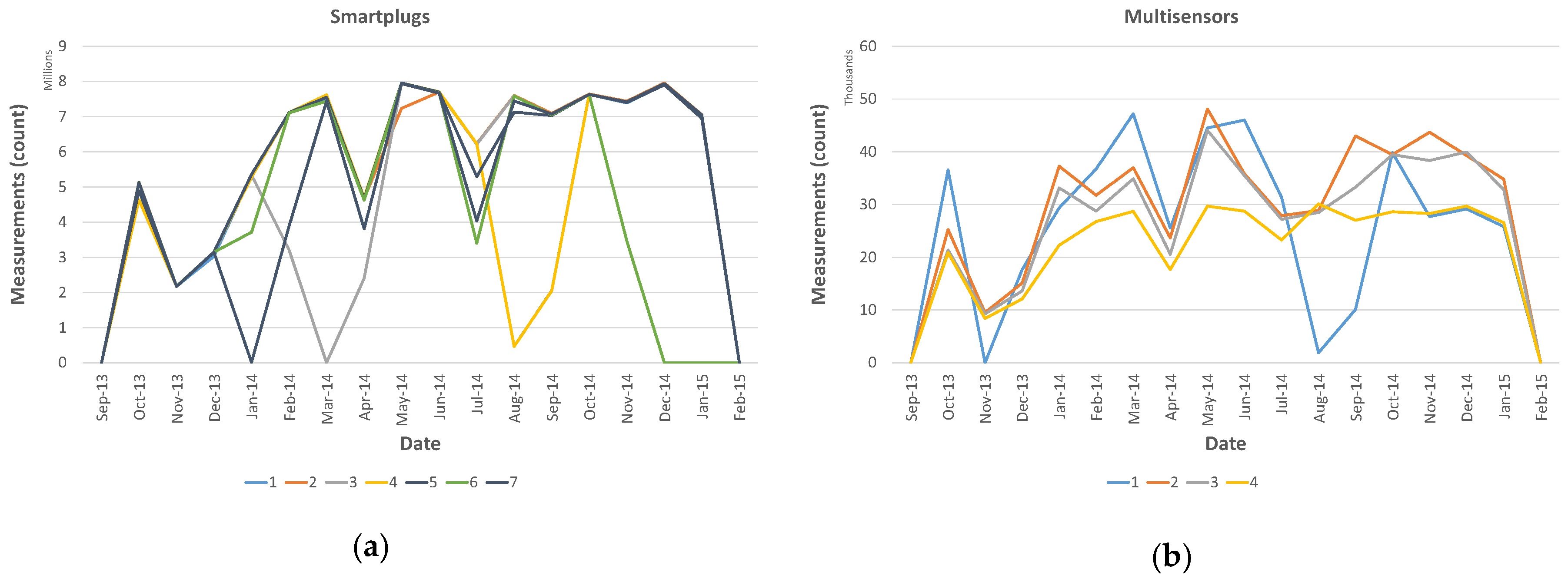
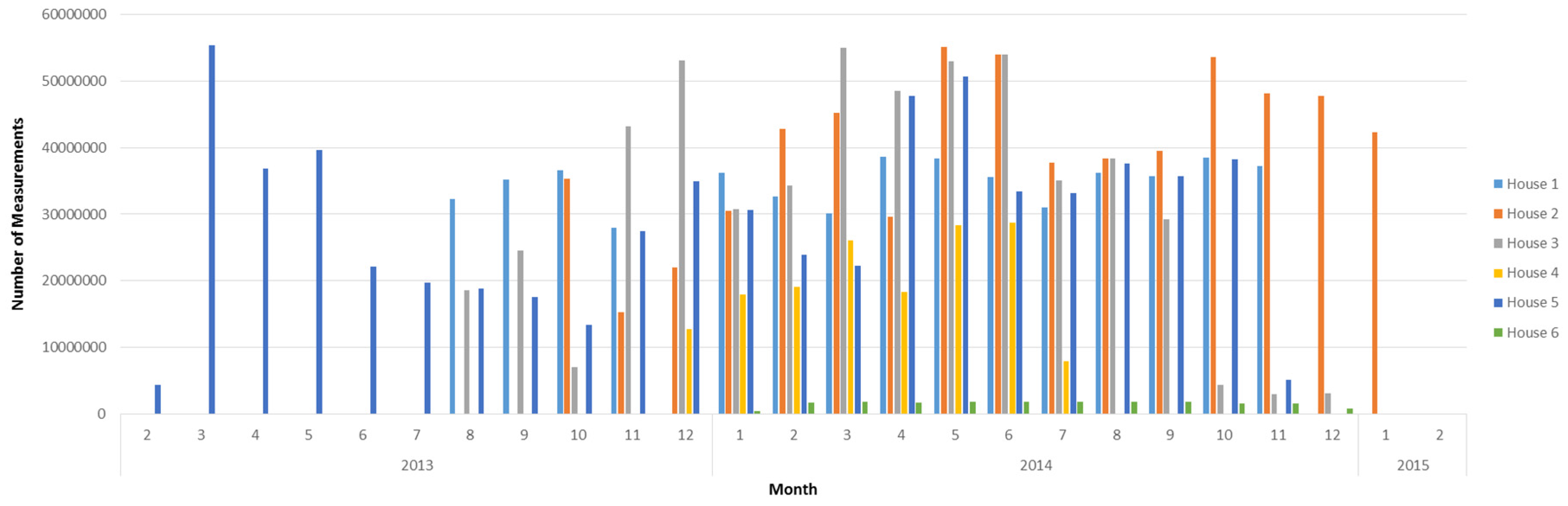
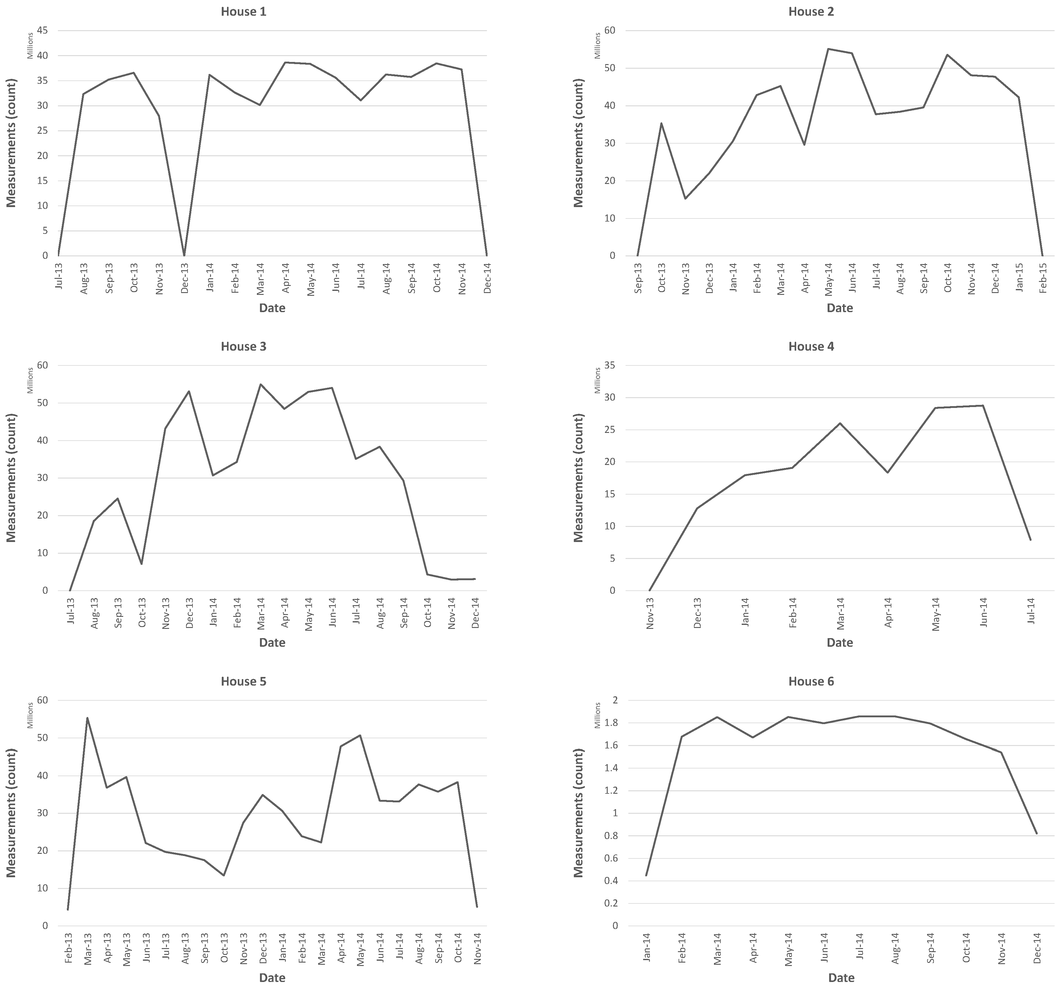
Figure 6 shows the aggregated number of measurements per month for each household.
In the following subsections, we first describe conversion errors of number and non-number types and then describe the data characteristics for each measurement type. Those measurement types that did not reveal any insights are not mentioned. For instance, we did not find any irregularities in the brightness readings.
4.1.1. Conversion Errors
All the measurements were initially stored as strings. As a first step towards assessing the data quality we validated the data types. Except for the on state of the smart plug and the battery state of the multi-sensor, values should represent floating point values. However 452 values could not be cast to a floating point. This affected all corresponding measurement types of the smart plug. None of the multi-sensors were affected by such parsing errors. In addition, there exists a single record of a current measurement where the actual measurement is completely missing (empty string). Of the non-floating point measurement types there were only two erroneous values of measurement type “on state”. The values were ONMS = 239 and ON6 and are likely caused by formatting errors in the sensor message or errors in the parsing process.
4.1.2. Work Anomalies
Ideally, work values would increase monotonically over time as the measurement was intended to represent the accumulated work since deploying the sensor. However, house occupants could reset the plug which would lead to reporting 0 kWh followed by monotonically increasing values. An event in which a preceding value was truly larger than the current value we therefore considered as anomaly. The overall number of anomalies is insignificant: out of the 421,589,929 work values only 17,876 anomalies were observed in our dataset. However we realized that only an insignificant part of the anomalies could have resulted from resetting the smart plug. The majority, i.e. between 98.19% and 99.99% of the anomalies per household showed as a non-zero drop in the work value. Our assumption is that this is due to network latencies that lead to messages arriving at the gateway out of order.
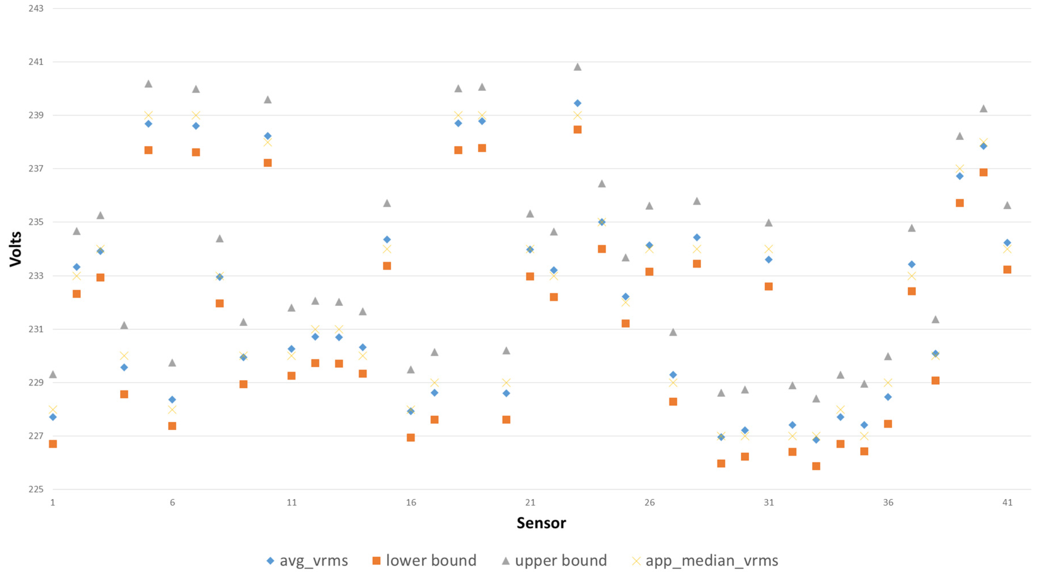
4.1.3. Voltage Anomalies
Figure 7 shows that most of the voltage values vary between 227 and 239 V and most values are around the average. We also looked at the minimum and maximum voltage values for each sensor in order to check whether they deliver plausible values. In terms of the maximum values (not shown in the figure) only two sensors exhibited unusual high values. One sensor reported a maximum voltage of over 1392 V whereas the second sensor reported 2099 V. Both sensors were deployed in House 3.
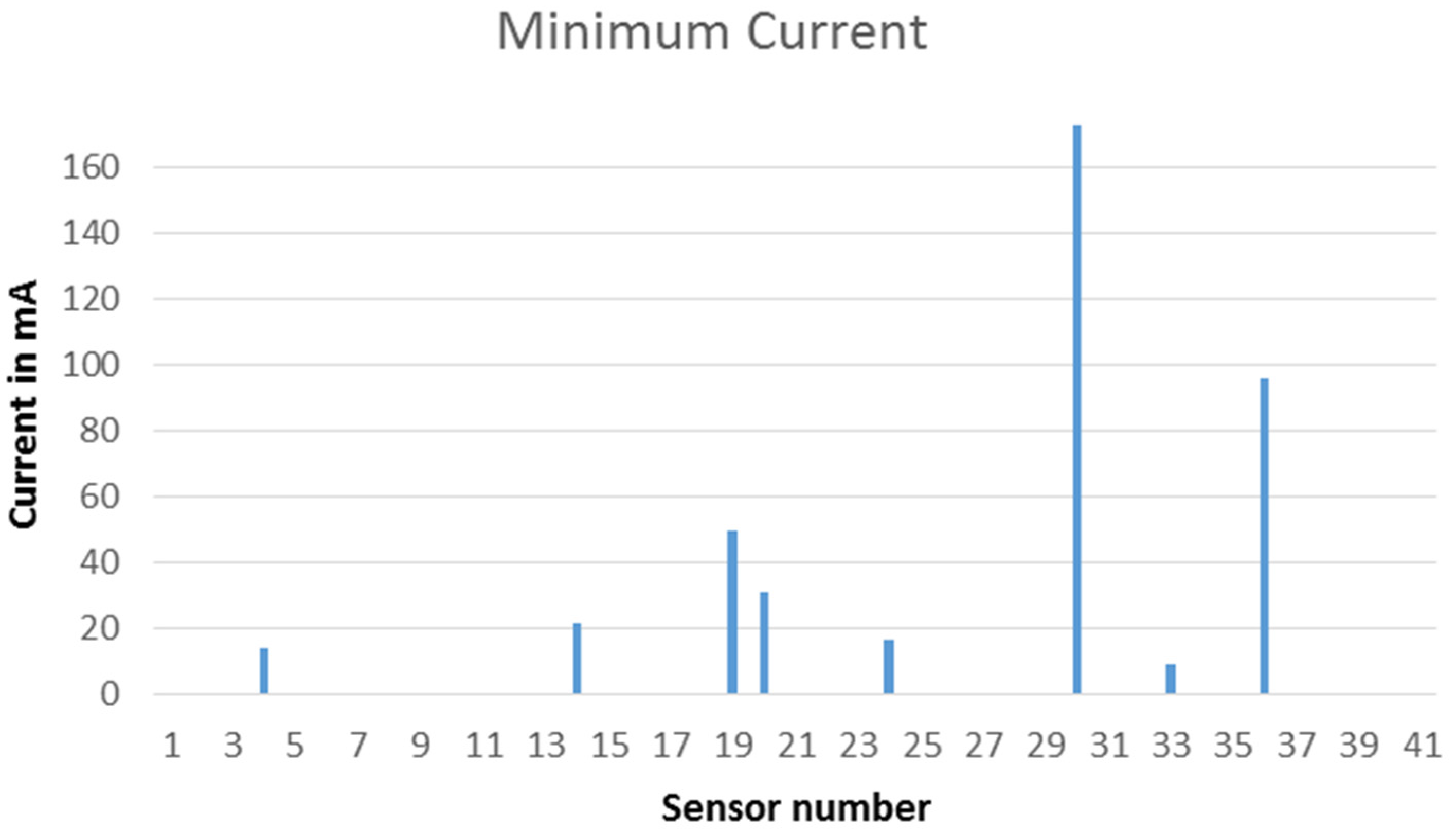
4.1.4. Current
When considering the minimum current measurements, it can be seen from
Figure 8 that for a majority of sensors,
i.e., 33 sensors, the minimum value equals zero. One sensor in House 6 reported an extremely high minimum value of 173.
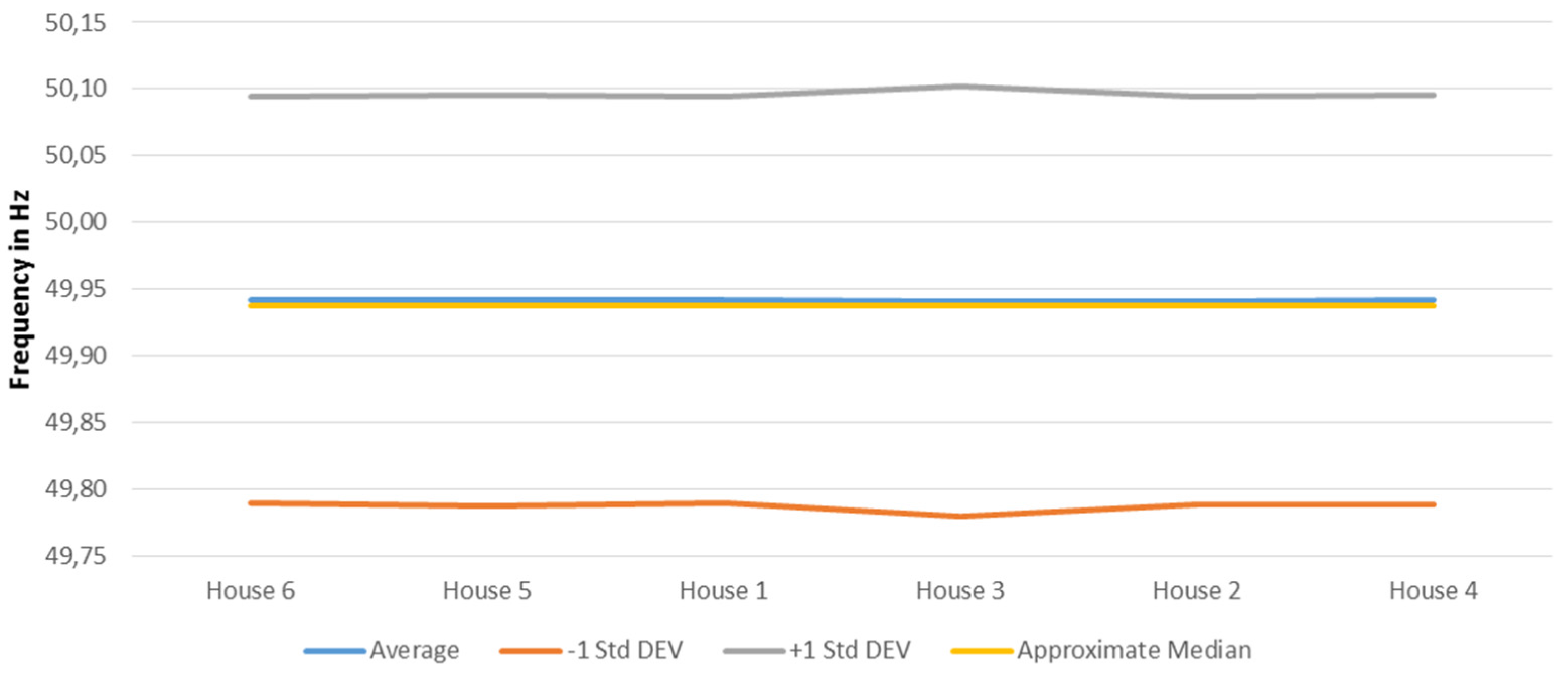
4.1.5. Frequency
As can be seen in
Figure 9 all the households exhibit a fairly homogenous statistical data characteristics. Average and median are both at 49.9 Hz for all households. The standard deviation is also very homogeneous at 0.15 Hz for all households. Only House 3 has a slightly higher standard deviation of 0.16 Hz which is mainly caused by the extremely high values reported by a single sensor.
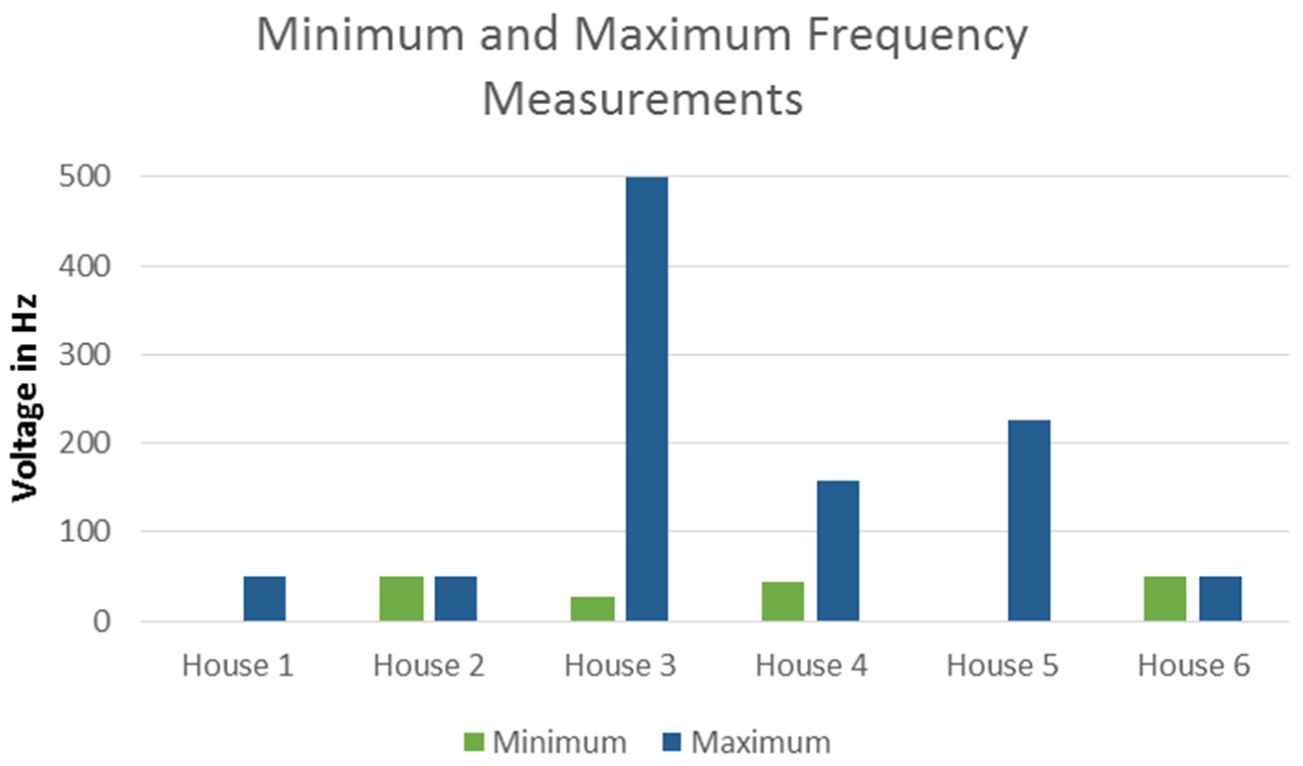
However, some anomalies are revealed when considering the maximum and minimum values as depicted in
Figure 10. Houses 1 and 2 do not exhibit any significant anomalies. House 1 shows values between 0 and 50.3 Hz and Houses 3 and 4 show irregularities both in the minimum and extremely high voltages.
A further drill down on the sensor level reveals that for House 5 the maximum value is caused by a single sensor) whereas the minimum is caused by another single sensor. A third sensor shows a minimum value of 12.1 Hz. All other sensors of House 5 exhibit have minimum values of 49.6 Hz and maximum values of 50.3 Hz. Similar observations hold for House 1. For House 3, the situation is slightly different as both the minimum and the maximum values are caused by a single sensor. This may be interpreted as a strong indication that the sensor is faulty. However there is also second sensor that has a maximum value of 238 Hz. Possible explanations for such value are sensor failures communication errors that cause the wrong measurements being interpreted as frequency measurements (e.g., 238 might actually be a voltage measurement).
The other sensors of House 3 provide values between 49.6 Hz and 50.3 Hz as all other sensors without outliers do. House 4 has two irregular sensors: one being responsible for the overall maximum and another one for the overall minimum of 44.5 Hz with a highest value of 63.3 Hz.
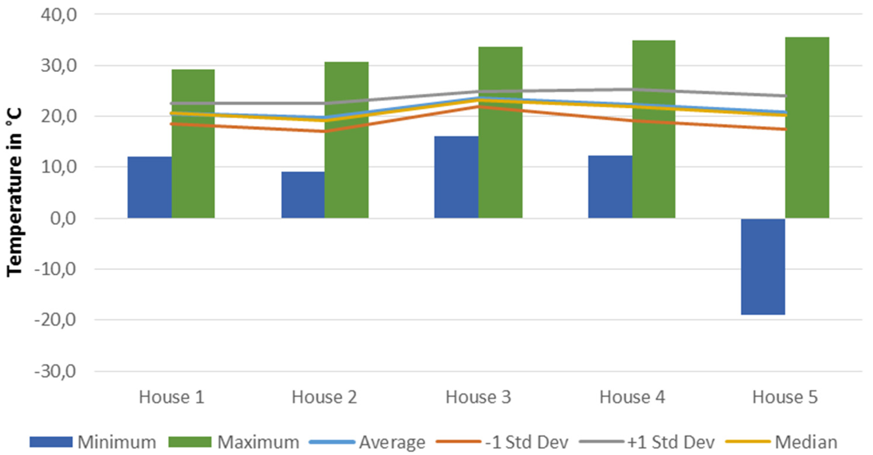
4.1.6. Temperature
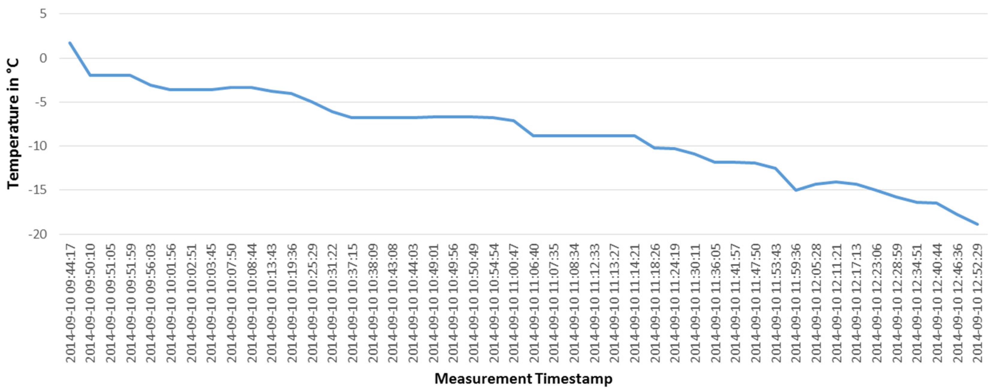
Temperature readings are not available for House 6 as no multi-sensors have been deployed in this household. Statistically, as can be seen in
Figure 11, the temperature readings provide plausible values being on average between 20.5 °C and 23.4 °C for the households. Also, the minimum and maximum values provide plausible results, but for House 5 the minimum value of −18.9 °C is unusually low. However, when drilling down to the time series of this sensor we can observe a continuous drop over 3 h (see
Figure 12). A possible explanation is that the sensor was put into a freezer. The multi-sensor containing the temperature did not report any other readings after the minimum temperature has been reported. So the device has not been reconnected to the gateway and may have even be rendered permanently damaged.
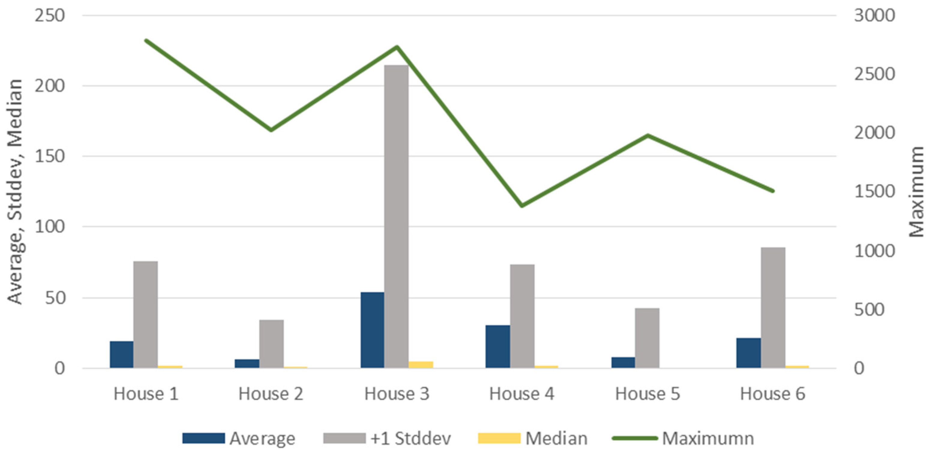
4.1.7. Power
As can be seen from
Figure 13 statistically the power readings follow the expectation. The average is moderately low between 8 and 54 W. Maximum values are between 1.5 and 2.8 kw reflecting high power consumers such as vacuum cleaners, fridges, or multi-sockets serving multiple devices. We would expect that there are only a few high power readings compared to the lower power readings. This is reflected by the small median and a higher standard deviation than the average.
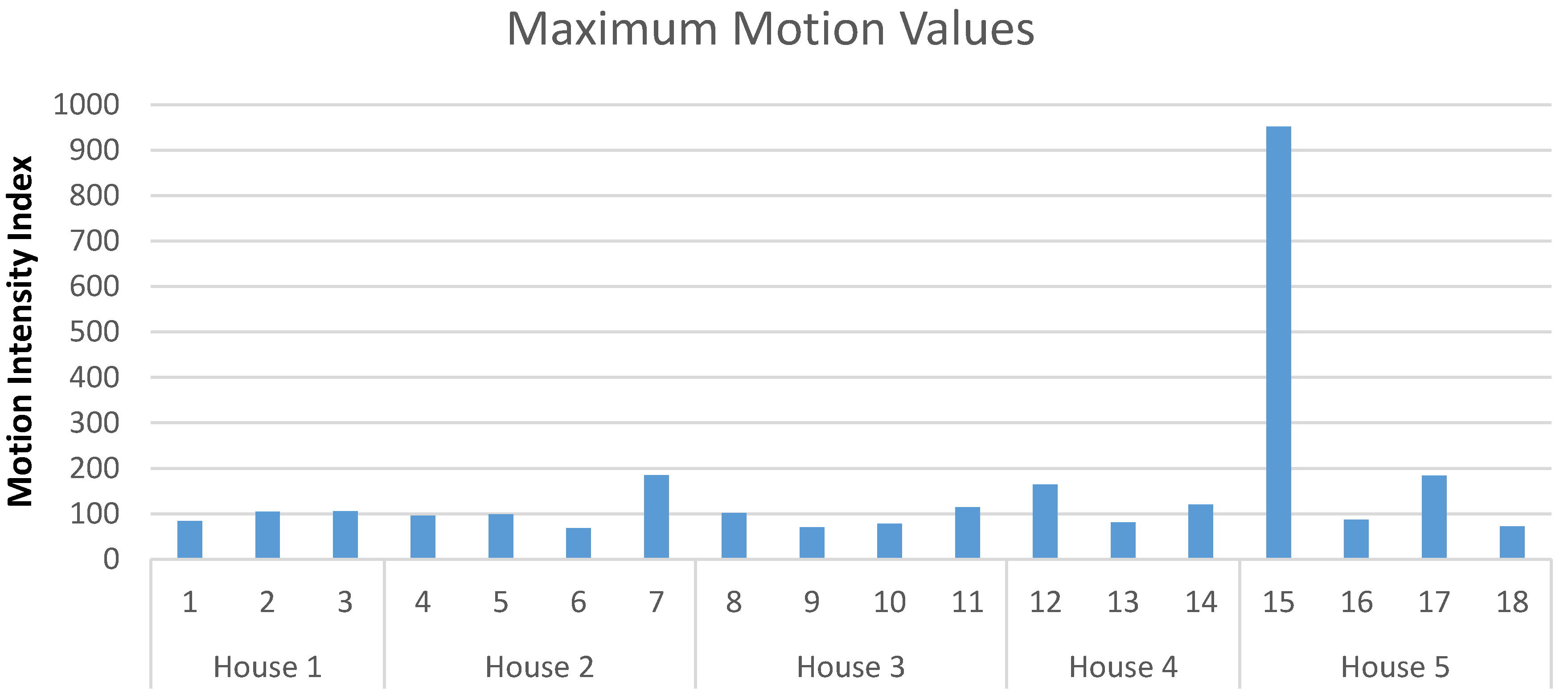
4.1.8. Motion Values
When considering the motion values (
i.e., the count of messages about detected motion), one sensor of House 5 show considerable higher numbers than the other sensors (see
Figure 14). A possible explanation for these high values could be that the sensor was deployed in a location that was exposed to direct sunlight.
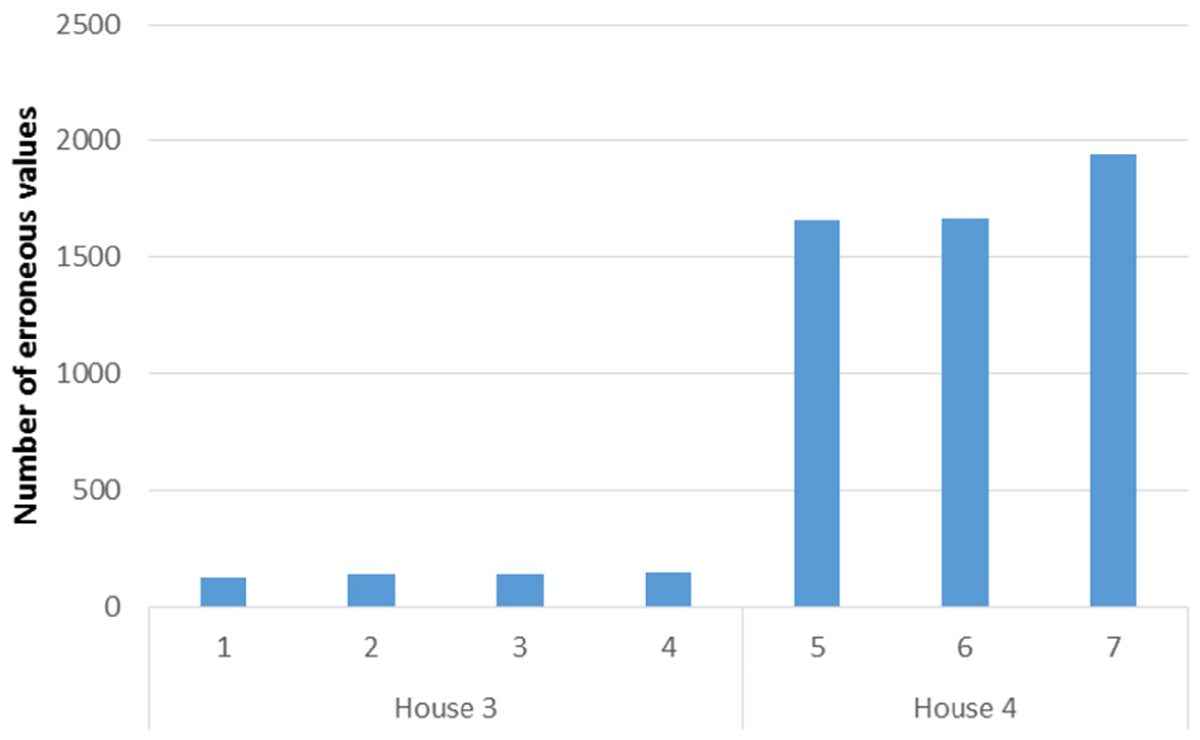
4.1.9. Battery Status
The battery status should only contain one of the two values LOW or OK. While 81.5% indicated a good battery status, only 18.1% indicated a LOW battery state. The remaining 0.3% constitute erroneous values. All erroneous values originated from two households and constituted floating point numbers in the range between 3.8 and 4.4, exclusively.
When drilling down on sensor level, we can observe that all deployed multi-sensors of both households reported erroneous values (see
Figure 15). More interestingly, we can observe that the number of erroneous measurements are very close together across the same sensors in a household. Noteworthy is also the fact that erroneous measurements only occur for each day in a timespan of seven days.
4.2. Arrival Rates of Sensor Data
All sensors in the pilot were configured to report data at a fixed sample rate. Thus, under ideal conditions, an application gets new data at a fixed rate. However, our experience from the pilot shows that data rates can vary significantly. In this section, we describe our analysis that provide insights into application level data rates that are achieved under real conditions. We ran separate analysis for the two different types of sensing devices that we employed in the pilot. The first type are the smart plugs that are get their energy from the power line and report new data every 2 s. The second type are the multi-sensors that are battery powered and configured to report new data every 6 min. Results for these two separate analyses are provided below.
4.3. Arrival Rates of Smart Plug Data
To analyze the application level data rates of smart plug data we use the application level time stamps in our data records. These timestamps are set for each new sensors record when it is received by the gateway and written into the local database. For the analysis we compute the recorded time difference between consecutive entries from the same sensor source. Under ideal conditions, this delay between consecutive values resembles the sample rate of the sensor. That is, we expect a new entry every 2 s. We compute the histogram of delays to understand if and how the actual arrival rates differ from the expected value.
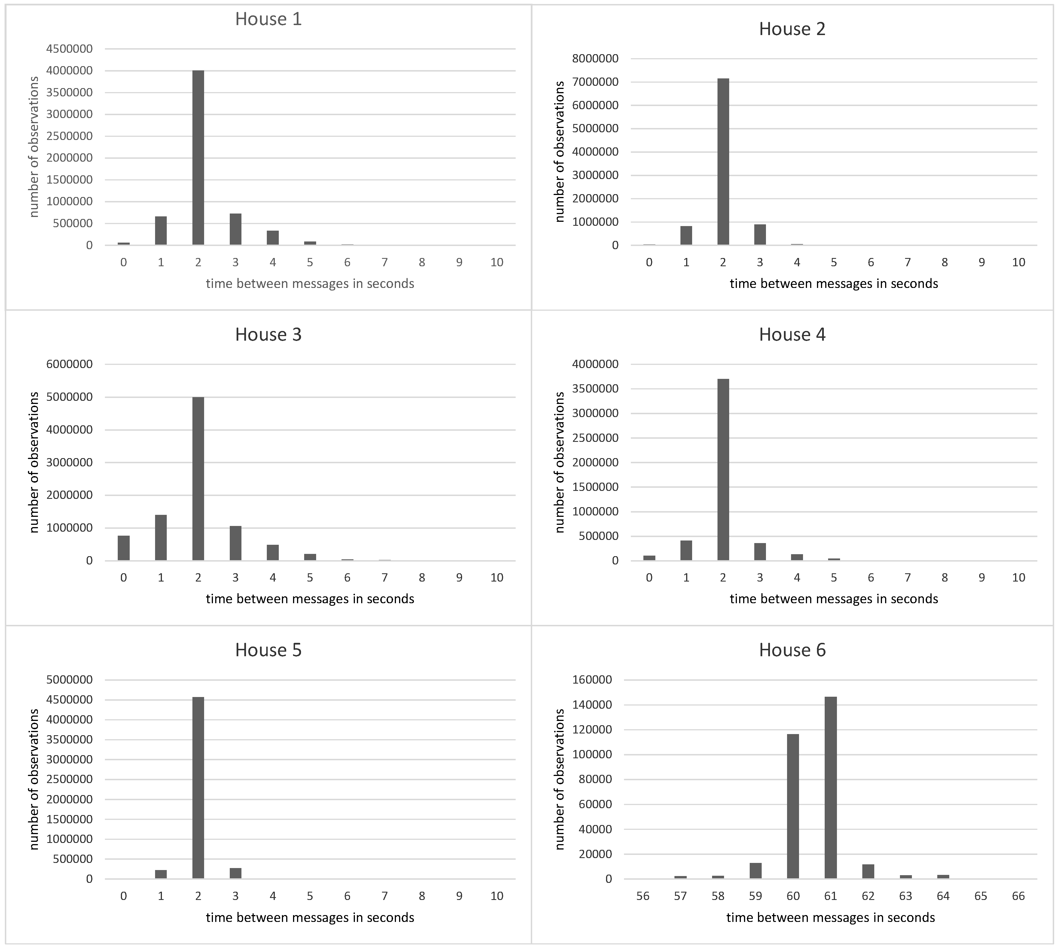
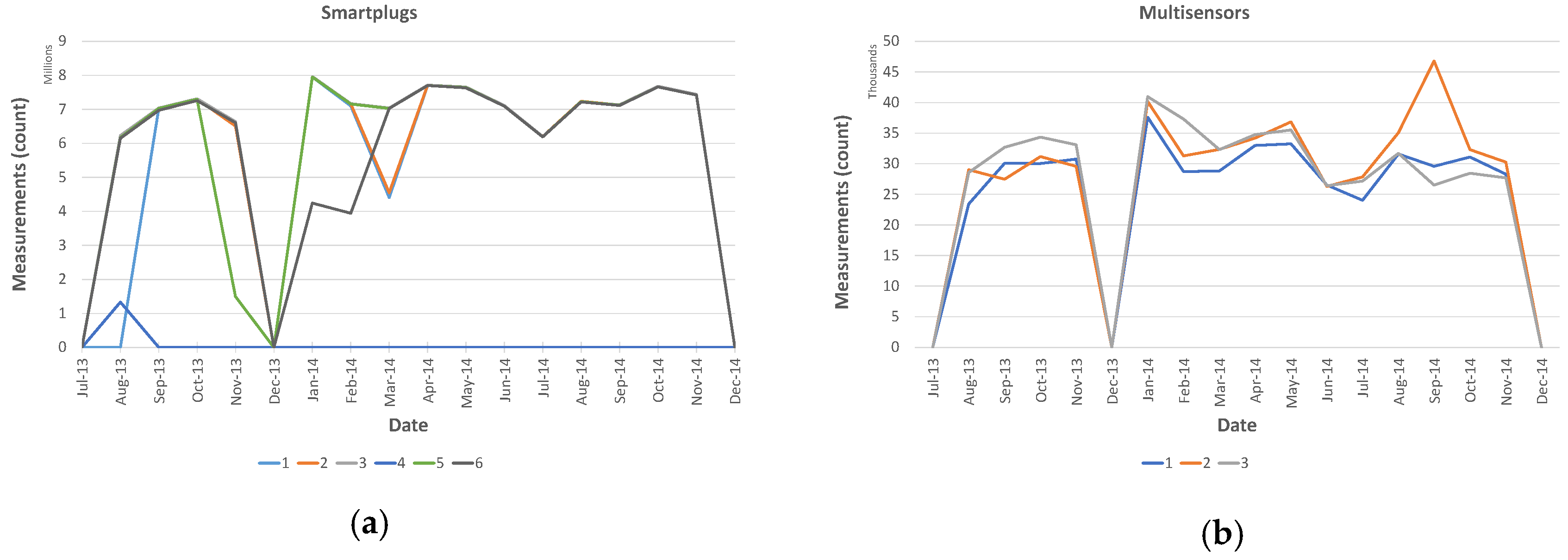
Figure 16 shows histograms of delays aggregated for all sensors in the six investigated houses. For the analysis, we used data of one month per house. Specifically, for all houses we took data from the same month in summer where all six houses were active in the pilot at the same time.
The results show, that the majority of delays are the expected 2 s in all but one case. The exception is House 6 where sensors were configured to sample once per minute. However, the histograms also reveal substantial deviations from the expected value at all houses. We observe several instances where consecutive messages are further apart than the sample rate defines. For instance, more than 11% of all computed time gaps were 3 s and 5% were 4 s at House 3. Also, several messages arrive in shorter intervals than the defined sample rate. In House 3, more than 8% of messages are recorded at the same time as their predecessors. More than another 15% of the messages are recorded with timestamps only 1 s apart.
The deviations can be seen at all houses. Yet, the magnitude of deviations differs among the installations. An obvious outlier is House 6, where the delays peak at 61 s. This is because the sensors in this particular house are configured to sample every minute. Yet, like in the other installations, we observe deviations from the expected value. Notably, the peak is at 61 s and not at the expected 60 s, indicating inaccuracies of the sensor clock. All other houses had the same configuration for the sensor sample rate. However, the magnitude of deviations varies among the installations. For instance, the histogram for House 5 shows most values at the expected 2 s interval with only few counts for 1 s and 3 s intervals. In contrast, House 3 shows comparatively large deviations from the expected values. Significant proportions of the messages arrive with considerably longer delays than expected, i.e., as long as 5 s or in some cases even above. Other messages arrive in shorter intervals, i.e., with 1 s delay or no measurable delay.
While long delays may partially be explained with dropped messages, the short delays show that messages travel with different speed through the network. These observations show clearly that specifics of the deployment environments in the different houses have a considerable impact on the arrival rates of sensors messages. Applications must be aware that arrival rates are not constant and the fact that this particular quality aspect varies between installations.
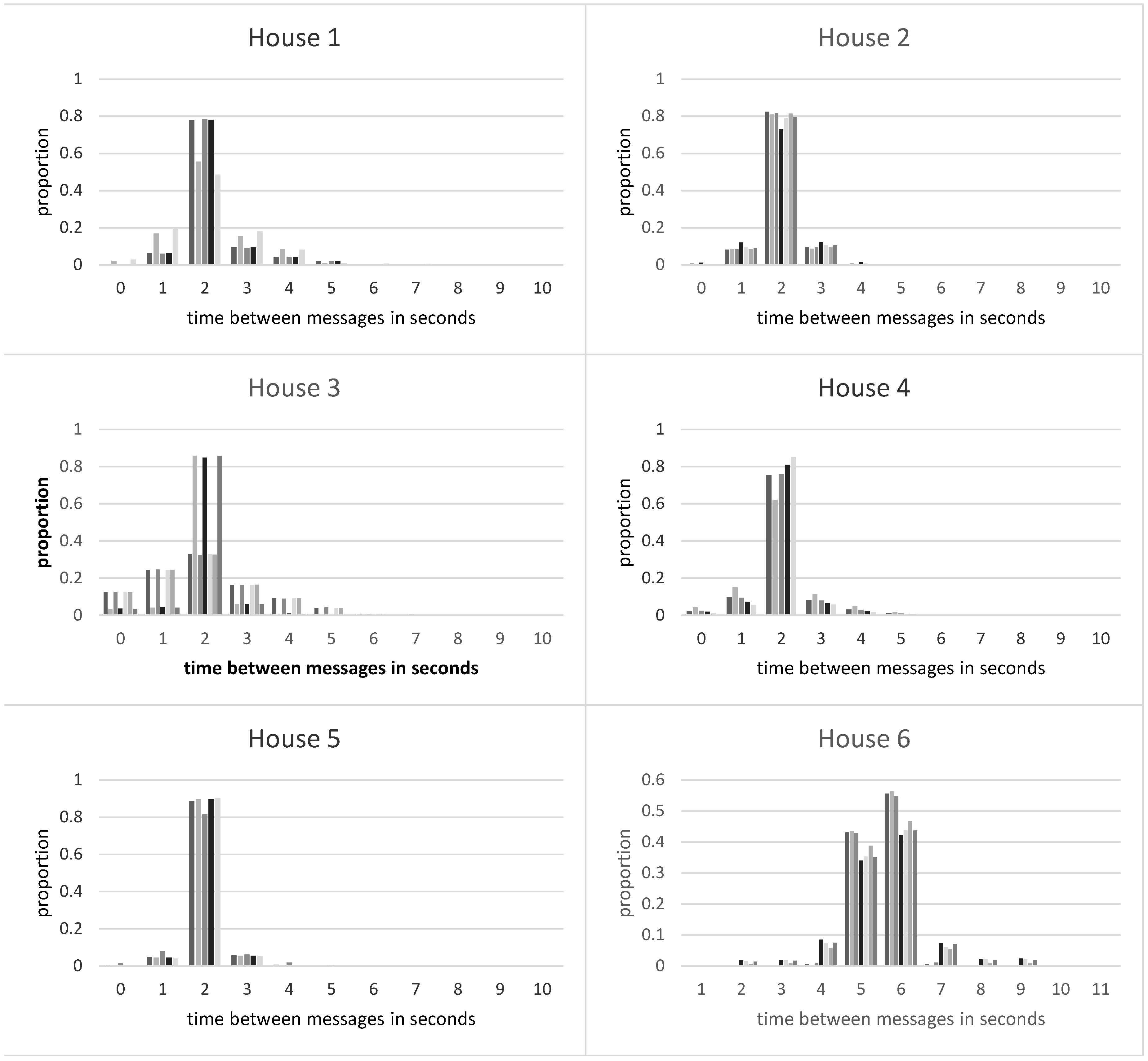
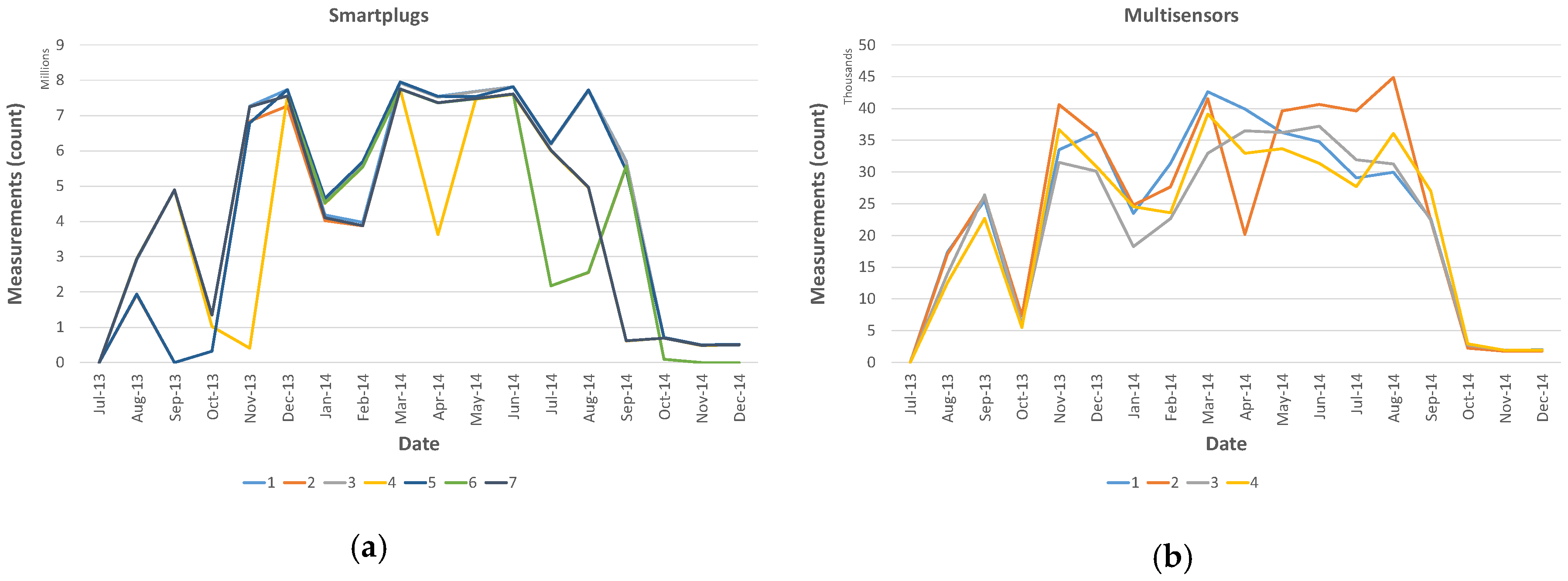
Figure 17 provides more details on the divergence of arrival rates, by drilling down on sensor level. As the figure shows, arrival rates of sensor measurements vary among sensors within the same house. For instance, in House 1 we observe that three of five sensors have very similar distribution for the arrival rates of their measurements. However, two sensors differ from that distributions. For these two sensors, the arrival rates divert considerably more from the expected two second interval. Similar, we observe two groups of sensors with similar distributions for arrival rates in House 3. Here, three of five sensors show similarly distributed and relatively large deviations from the expected value. The other two sensors show only few and small deviations. Compared to each other, the corresponding distributions for these two sensors are also very similar.
In particular, for House 3 it is notable how the distributions of arrival rates fall in two very distinct groups. It is therefore likely that the larger deviations in arrival rates have the same or similar cause for all sensors. A possible explanation is multi-hop communication in the ZigBee network. Some sensors have a direct connection to the gateway while others get their messages relayed by a neighbor sensor. Communication via one hop is potentially more error prone than direct communication. Another possible explanation is that the different groups of sensors are situated in different physical conditions. That is, a group of similarly performing sensors may be deployed in the same room, having to communicate through the same walls to the gateway.
Table 3 provides an overview of the gap distributions of gaps sizes per house and sensor with regards to the variance. Note that we removed rare outliers (
i.e., with only a single observation in the whole data set) from the computation. For the expectation value we took the sample rate of the corresponding device. In summary, we find that a considerable proportion of sensors shows low variance in arrival rates (between 0.32 s and 1 s), while a smaller proportion yields high variance (between 1 s and 10.83 s). Each house has at least one sensor with a variance below or up to one second. However, the overall variance differs significantly due to the different numbers of sensors with high variances in the deployed portfolio.
4.4. Arrival Rates of Multi-Sensor Data
Similar as in the analysis for smart plug data, we use the application level time stamps in our data records to analyze the application level data rates of multi-sensor data. Like for the smart plugs, these timestamps are set for each new sensors record when it is received by the gateway and written into the local database. Unlike smart plugs, the multi-sensors are battery powered. We chose a sample rate of one sample every 6 min to ensure a sufficient battery life time (
i.e., more than 6 months with one set of batteries). For all houses we took data from the same month in summer. Like for smart plugs, we compute the recorded time difference between consecutive entries from the same sensor source to analyze arrival rates on application level. Under ideal conditions, this delay between consecutive values resembles sample rate of the sensor. That is, we expect a new entry every 6 min. To understand how the actual arrival rates compare to the expected value we count for each observed delay how often a delay of that length occurs (with a time resolution of one second).
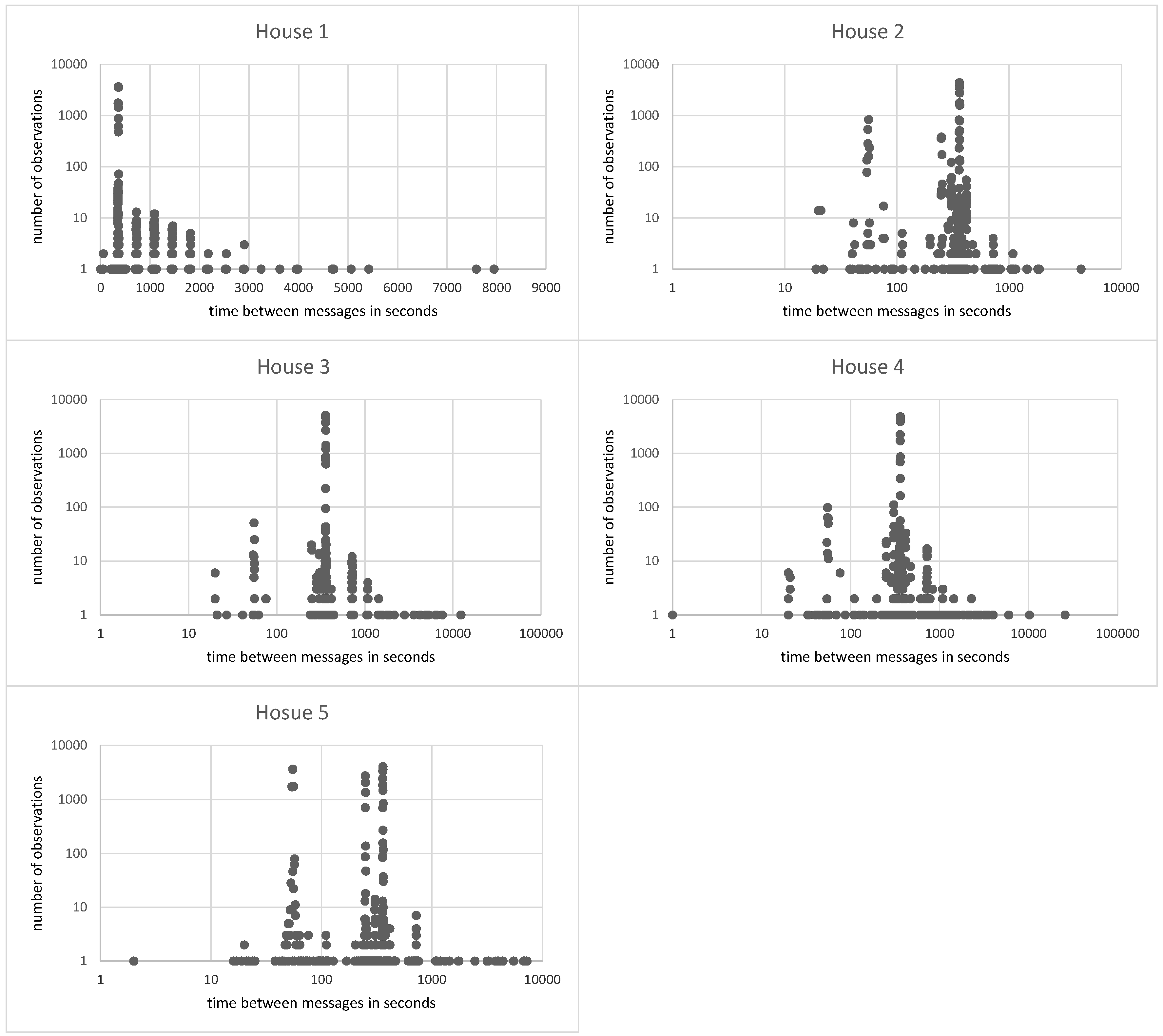
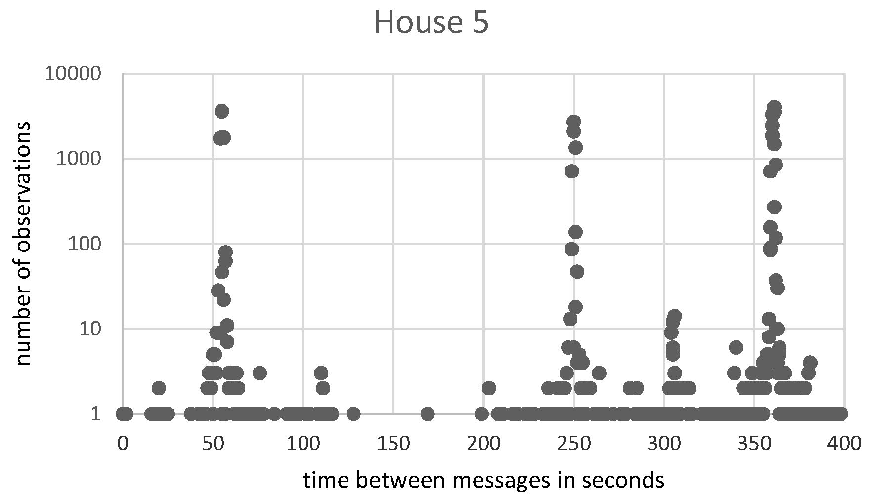
Figure 18 visualized the results as scatter plots.
The x-axis reflects the delay duration and the y-axis marks the observed count for each delay. House 6 is missing from the analysis because no multi-sensors were available in this installation.
As
Figure 18 shows, the observed arrival rates differ significantly from the expected 6 min. The delay values with the highest count are about 6 min for all houses (361 s in most cases), but a substantial number of observations deviate from that value by several seconds or even minutes. Also, in the vicinity of the expected value we observe high counts for values that are several seconds off from the expected 6 min.
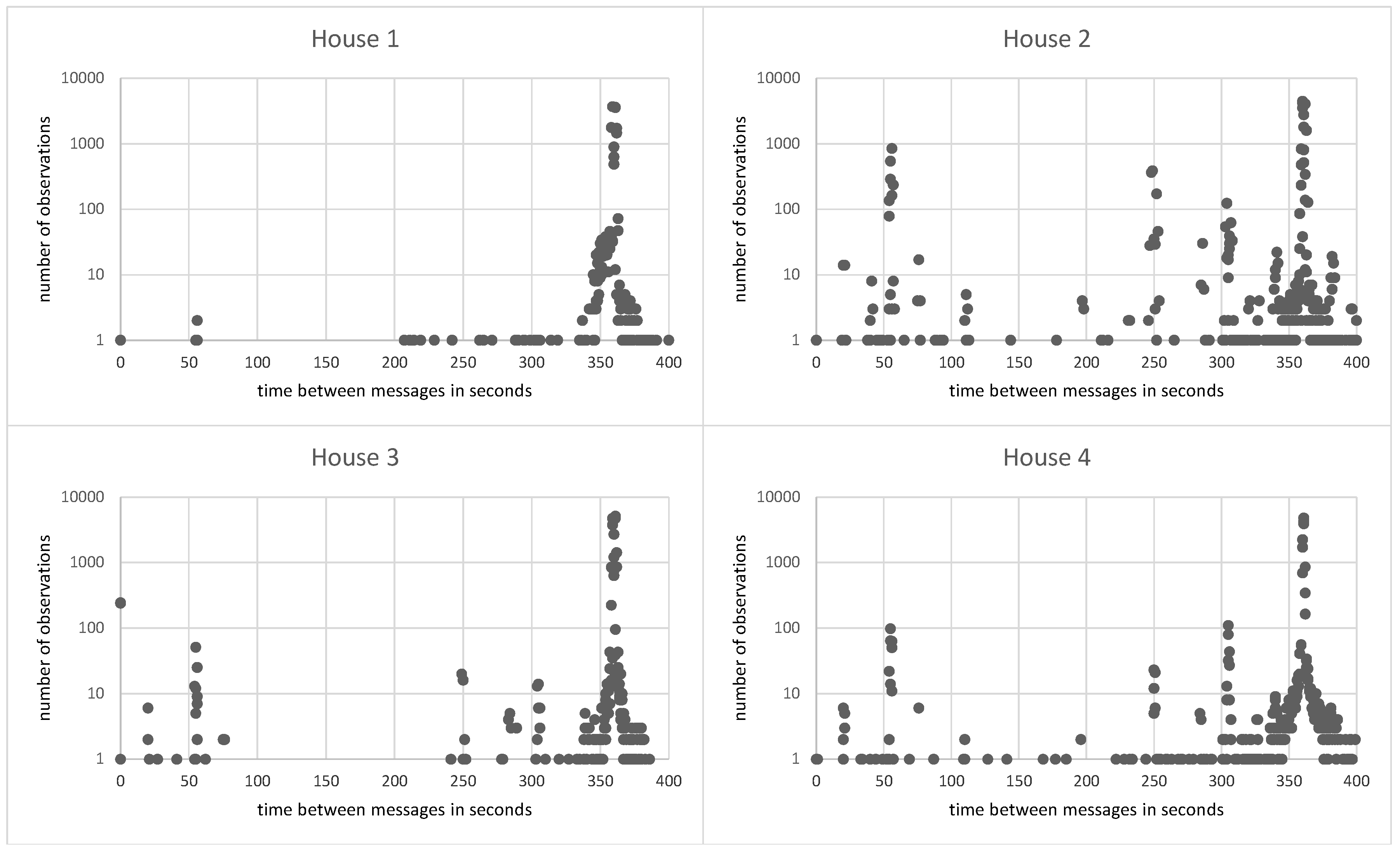
Figure 19 details the analysis of these deviations by zooming in on the time-axis. The figure shows several occurrences where the time between message arrivals is tens of seconds shorter or longer than expected. The order of magnitude and frequency of these deviations is notably higher than for the smart plugs.
The overview in
Figure 18 further reveals that the time spans between consecutive messages accumulate around certain values. For House 1, we observe high counts for values that are roughly multiples of 6 min. Such a pattern is expected as results for lost messages. Notably, House 1 is the only house were such patterns materialize. For the other houses we do not observe accumulations around the multiples of 6 min. That means, drop rates were overall low in 4 of the 5 analyzed cases. However, at all houses we do find accumulations at values that are not multiples of the sample rate. In particular, some spikes can be seen for values around one minute, 250 s. These patterns cannot be explained by dropped messages and are assumed to be a result of hardware properties of use sensors. Overall, the analysis shows that time spans between consecutive messages are scattered across large ranges. This leads to rather unstable arrival rates that must be accounted for by applications that use the data.
4.5. Downtimes of Infrastructure Components
In this section, we analyze the behavior of the gateways during the months they were supposed to be active. Specifically,
Figure 20 shows the behavior of each gateway in terms of cumulative number of measurements received per month. As the figure shows, the behavior is very different every month. In order to understand the reason, we report from
Figure 21,
Figure 22,
Figure 23,
Figure 24,
Figure 25 and
Figure 26 also the number of measures received from sensors and smart plugs separately, so this can help us to identify when the gateway was down or when some devices were disconnected from the gateway causing a drop on the measurement count.
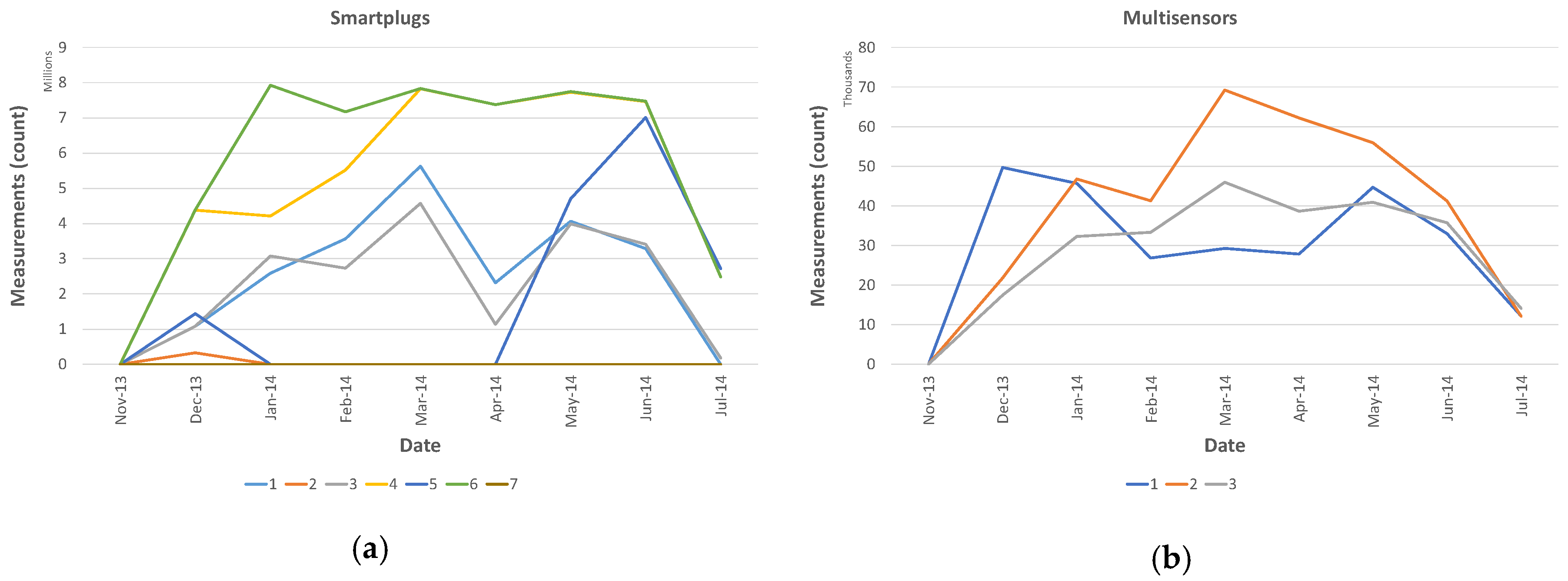
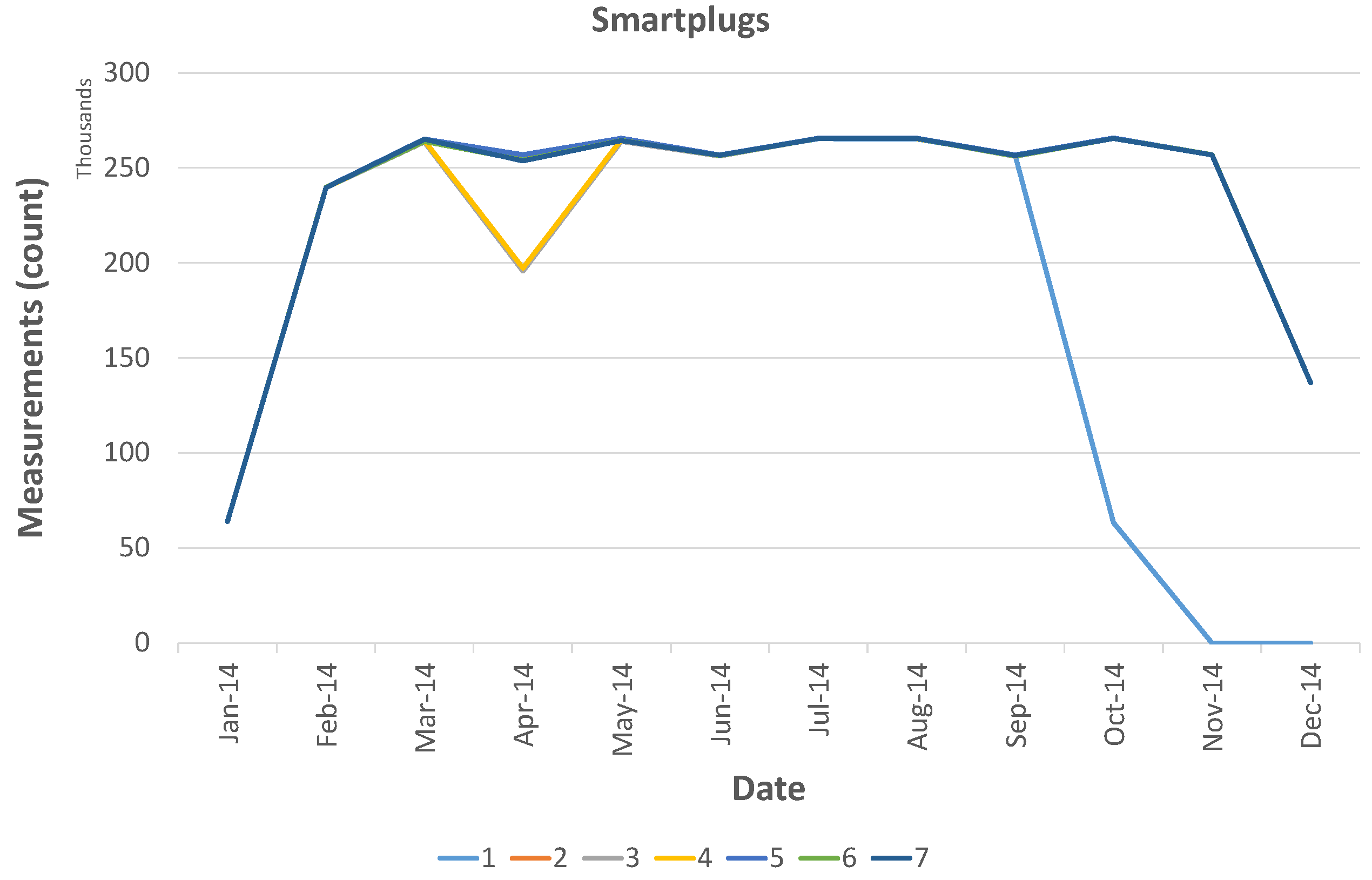
Looking at the figures, it is clear that the gateway of House 1 went down in the last part of November till December 2013 maybe due to some power issues or an operating system crash. It was rebooted in January 2014. Apart from Smart Plug 4 (that was on only some days in August 2013 and off all the other months) all the other devices in House 1 reported results with a very close frequency.
House 2 presents a behavior that changes during the months. We note a minimum in November 2013 where the gateway was disconnected for several weeks and all the devices reported a low number of values. The other minimum value was in April 2014 for the same reason. Instead, in August 2014 we observe that both a smart plug and a multi-sensor were disconnected for several days. This can be related to a disconnection in the ZigBee network due to the removal of the smart plug and consequently disconnection of the multi-sensor that used that specific smart plug to reach the gateway.
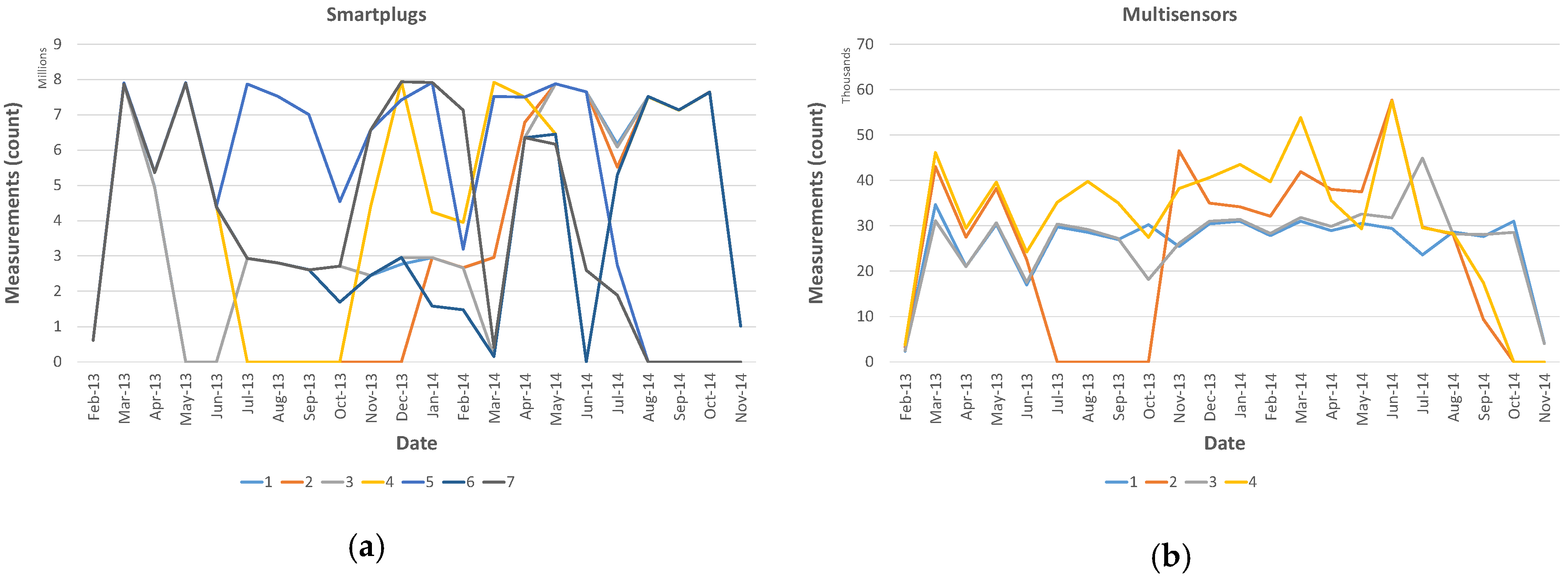
The Gateway of House 3 was down three weeks in October 2013, then it was rebooted. In January and February 2014, it was on only for half of the time. Also in this case the motivation can be a power failure or a crash in the operating system. We note also that, in August and September 2013, the data collected are less with respect to the other months. This can be due to a not very stable connection of the network at the beginning. The same happened in September and October 2014 before dismissing the Gateway, due to the fact that probably the user started to disconnect the smart plugs causing a disruption in the ZigBee network.
House 4 presents a ramp-up in the number of data collected maybe due to the fact that the number of devices increased over the time. Two smart plugs reported very few measurements at the beginning and one was off most of the time. We note a minimum in April 2014, this was not caused by a malfunction of the gateway, but due to two smart plugs that reported few values.
House 5 is characterized by a very unstable environment. The number of measurements reported by both smart plugs and multi-sensors changes a lot due mainly to the weak network connection or the location change of the devices. The gateway itself seems to behave correctly.
House 6 is characterized by having only smart plugs, but here the number of measurements collected is quite constant due to a more stable network connectivity and a more stable topology.
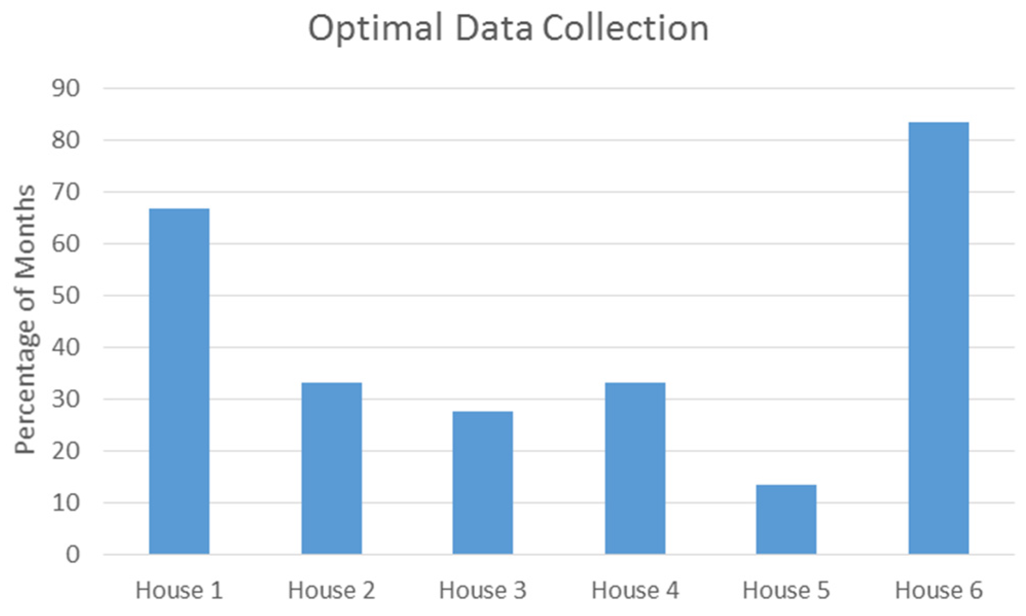
To have a comprehensive view of the behavior during the months of observation, in
Figure 27 we present a graph showing the percentage of months where we registered an “optimal data collection” per house, quantified as a number of months (in percentage over the total) with a collection volume greater than 80% of the maximum volume. Only Houses 1 and 6 had more than 60% of the total months more than 80% of the maximum volume of data collected.
Overall the results show, that continuous connectivity must not be expected in the described setting. The physical deployment on site is out of the control of the system operators and home owners may handle the system with varying degrees of care or intentionally temporary disconnect the system (e.g., to plug some other device in the used network socket). The reasons for human-induced disruptions are manifold and depend on the individual household inhabitants as well as on their living situation. For instance, we learned about incidents where the network cable was accidentally disconnected while cleaning the house, kids disconnected the plugs while playing, or the internet connection is generally unstable.
Applications that use the data must be aware that the data collection happens in an uncontrolled environment and availability of the components inside the households cannot be ensured.
5. Related work
According to our knowledge, several systems integrating sensor networks with energy management systems at the consumer premises have been proposed so far. The closest to our project is Linear [
7], a Flemish Smart Grid project focusing on solutions to match residential electricity consumption with available wind and solar energy, an approach referred to as demand response. The project suffered from the amount of data and transactions collected since no big data technologies to handle that were used. Additionally, in-house communications were one of the major sources of technical malfunctions. Linear installed, on average, 11 ZigBee plugs in each home, half of them serving exclusively to bridge communication signals. Linear preferred “Ethernet over PLC to Wi-Fi “for connecting the different modules in the house with the gateway. This choice quite often caused conflicts with existing applications such as the home network and digital television. According to the Linear support team, “some families were so excited about the possibilities of the Home Energy Management System that they started moving plugs to different locations in order to trace standby losses, not being aware that they were messing up the network to the extent that the fridge plug started showing the behavior of a television in our databases”. Similar issues have been experienced also in our pilot as described earlier.
Another set of related projects was conducted as part of the e-energy funding scheme of the German government [
8]. For instance, the MeRegio conducted a pilot, mainly focused on using smart meter data [
9] and the project Smart Watts addresses the development of communication standards [
10]. However, to our knowledge, none of these projects provide detailed insights on the data quality aspect for smart home applications.
In [
11], the authors evaluate the performance of an in-home energy management system based on a ZigBee wireless sensor network. The focus there is the performance of the system on the application level, meaning the investigation of the potential of both energy management and demand management. The evaluation that has been performed by the authors is based on simulation results, and not on real network deployments in households as in our work.
In [
12], energy management in homes has been investigated on a pilot consisting of only three households in Sacramento. The solution has been implemented using off-the-shelf components based on power line communication, and it included a web-based monitoring and control of home appliances. Similarly, the MIT provides a detailed dataset with plug-level energy data [
13]. However, the dataset is designed to drive research on energy disaggregation and not to understand data quality issues under realistic conditions. Also, it is limited to a few weeks of recorded data.
In [
14], the authors present experiences from a pilot study carried out in Norway, focusing on daily demand response from households, utilizing smart metering, remote load control, pricing based on the hourly spot price combined with a time of day network tariff, and a token provided to the customers indicating peak hours. The pilot study has shown that household customers through simple and predictable means can adapt their electricity demand to the market situation.
6. Conclusion and Lessons Learned
In this paper, we have provided insights from a three year pilot with a cloud-based test bed for capturing and analyzing smart-home data. Our results include findings on real-world challenges in the application domain as well as our learnings regarding the data quality issues we have faced. The key challenge that we came across was data loss and reduced data quality on several layers of our cloud-based architecture. In many cases, the issues are inherent to the application domain which we were addressing (home environments) where users intentionally or unintentionally interfere with the operations of the system, but apart from this unavoidable problem we have presented a detailed analysis of the main causes that are responsible for data quality related issues.
In our tests, we quantify the data quality of a real-world smart home deployments and show how errors in such an environment are characterized. The derived characteristics concern (a) data errors; (b) arrival rates; and (c) behavior over time. Regarding (a) data errors we found that these occur only rarely. For instance, only 0.004% of measured work values showed a detectable anomaly. However, due to the overall high number of measurements, the total amount false data reaches high numbers. For instance, overall 17.876 faulty values were detected in the measurements of work.
Regarding (b) arrival rates for smart plug data we found significant variations across sensors. The analysis show variance values between about 0.32 and 2.5, for plugs with a sample frequency of 2 s. For the setup with sampling once per minute, we observe a variance of about 4.9. The overall variance differs significantly (i.e., between 0.49 and 4.85 s). However, we found in each house sensors with low variance (i.e., up to 1 s). Thus, we can conclude that ideal communication conditions allow for low variance in arrival rates, yet most real world setup will cause high variance in data arrival for at least some sensors in the portfolio.
Regarding (c) system behavior over time, we found that under real world conditions data quality changes considerably over time. We observe several drops in the overall measurement rate, both on the gateway and on the sensors level. Overall, only a third of the analyzed houses close to optimal reporting rates more than 60% of the time.
Overall, our work shows researchers as well as practitioners in the smart grid domain what challenges they have to expect when integration smart home technology and provide quantified insights into data quality in that domain. The findings support the design of systems and applications that cope with the data challenges and fuel future research on improving data quality for smart homes.


