Towards Sensor-Actuator Coupling in an Automated Order Picking System by Detecting Sealed Seams on Pouch Packed Goods

Abstract

In this paper, a novel concept of coupling the actuators of an automated order picking system for pouch packed goods with an embedded CCD camera sensor by means of image processing and machine learning is presented. The picking system mechanically combines the conveyance and singularization of a still-connected chain of pouch packed goods in a single machinery. The proposed algorithms perform a per-frame processing of the captured images in real-time to detect the sealed seams of the ongoing pouches. The detections are used to deduce cutting decisions in order to control the system’s actuators, namely the drive pulley for conveyance and the cutting device for the separation. Within this context, two controlling strategies are presented as well which specify the interaction of the sensor and the actuators. The detection is carried out by two different marker detection strategies: enhanced Template Matching as a heuristic and Support Vector Machines as a supervised classification based concept. Depending on the employed marker, detection rates of almost 100% with a calculation time of less than 40 ms are possible. From a logistic point of view, sealed seam widths of 20 mm prove feasible.

1. Introduction

Typical logistic processes like order picking became significantly more complex and dynamic during the last years. This is mainly driven by increasing e-commerce (e.g., estimated growth of 24.8% in 2014 in Germany only [1]) and reduction of buffer stocks in production lines. Obviously, this also affects the logistics of companies considerably. On the one hand, the number of shipments (packages) rises while the number of items (goods) per shipment declines. To face the required needs in e-commerce fulfilment and production industry as well, automated solutions are desirable because they typically reduce costs and failure rates when compared to manual handling. Especially in the business sectors Distributive Trades with 6.144 enterprises in Europe and “Transport and Storage” with 1.118 enterprises in Europe, a significant sales market for automated solutions is given [2].

However, the automated handling of non-rigid packagings (like plastic pouches) are still challenging due to their mechanical and geometric properties. In spite of the disadvantages of plastic pouches like, e.g., missing stack-ability, lack of shock absorption, unpredictable position, shape, and reaction to forces, they do have certain advantages such as low prices, space-saving storage, lightweight, hygienic properties, and transparency. These make them an attractive alternative to other packages like cardboard packages and support their wide-spread use in the industrial and end-consumer sector; sometimes, pouches may even be the only available packaging choice [3]. In the fourth quarter of 2013, around 5.100 machines for tubular or side-sealed pouch packages with a business volume of more than 103 million Euros [4] were produced in Germany only. Hence, a potential market for automated pouch handling solutions exists, too.

The aforementioned disadvantages impede the automated handling of pouch packed goods considerably. This paper presents a possible solution to handle such goods in an automatic way; an overview of the utilized hardware is given hereafter. At the Fraunhofer Institute for Material Flow and Logistics, preliminary work concerning automated order picking of pouch packaged goods has been accomplished. In several research projects, mechanical and analytical models have been developed and assessed [3] which finally led to a prototype of an automated order picking system. It offers a possible solution to the conveyance and separation of pouch packed goods in a single machinery. The basic idea of the system can be summarized as follows: Pouches are produced and stored as a chain to simplify subsequent handling operations. For order picking, the pouch chain is loaded into the machine, the chain is automatically fed forward by a cover band drive, cut into single pouches, and dispensed to full customer order lines. Inherent to the functional principle of cover belt conveyors are almost random variations of the pouch geometry during conveyance caused by the fillings of the pouches. This leads to different heights of the pouches and, hence, accurate determination of the feed distance is impossible due to pouch deformations and varying friction between the belt and guide pulley. From the mechanical point of view, dimensioning and design of the order picking system have been researched in the past but, finally, an efficient and inexpensive solution for the cutting line (sealed seam) detection was missing to empower the system to automatically separate the chain of pouches according to given customer orders.

Within this paper, a novel concept of coupling the actuators of the picking system (a servo eccentric drive for conveyance and the cutting device) with an embedded CCD camera (-sensor) by means of image processing and machine learning is presented. More specifically, captured images are used for the detection of the cutting lines which, in turn, are used for deducing the final cutting decision. Besides the detection algorithms, two controlling strategies are introduced which determine the specific interaction of the sensor and the actuators. Clearly, the presented concepts may also be applied in identification and automation processes different to the underlying picking system utilized in this paper since they cope with the general challenges superimposed by the disadvantages of pouch-packagings.

Employing a vision based solution enables a high flexibility concerning different packaging materials (foils), types of pouches, fillings (i.e., packed goods), and markers. Decreasing prices for cameras and computers in combination with applied software solutions offer an economical alternative to specialized one-purpose sensor solutions.

The rest of this paper is organized as follows. In Section 2, State of the Art is presented for automated order picking, different pouches in the industry, and today’s solutions for cutting line detection. Section 3 describes the setup of the automated order picking system and its components. The core of this paper—the novel marker detection methodology to interface the actuators—is described in Section 4. Section 5 deals with an experimental assessment of the presented algorithms in terms of detection quality, cutting accuracy and runtime using the real machine setup of the order picking system described in Section 3. Finally, Section 6 summarizes the main statements of the paper and concludes with an outlook on future work.

2. State of the Art

Due to the constant need of automation in production, order picking and warehousing, a wide range of technical solutions have been developed over the last 20 years. The following sections show the state of development in the field concerning this work. More specifically, Section 2.1 reviews existing automated solutions and examines whether they can be used for automated order-picking of pouch-packed goods. Additionally, the presented picking system is differentiated from existing systems and a usage scenario is revealed. Section 2.2 surveys different types of pouches used in industrial systems. Finally, Section 2.3 explains typical hardware systems employed for cutting line detection and how they can be utilized for the purposes of this paper.

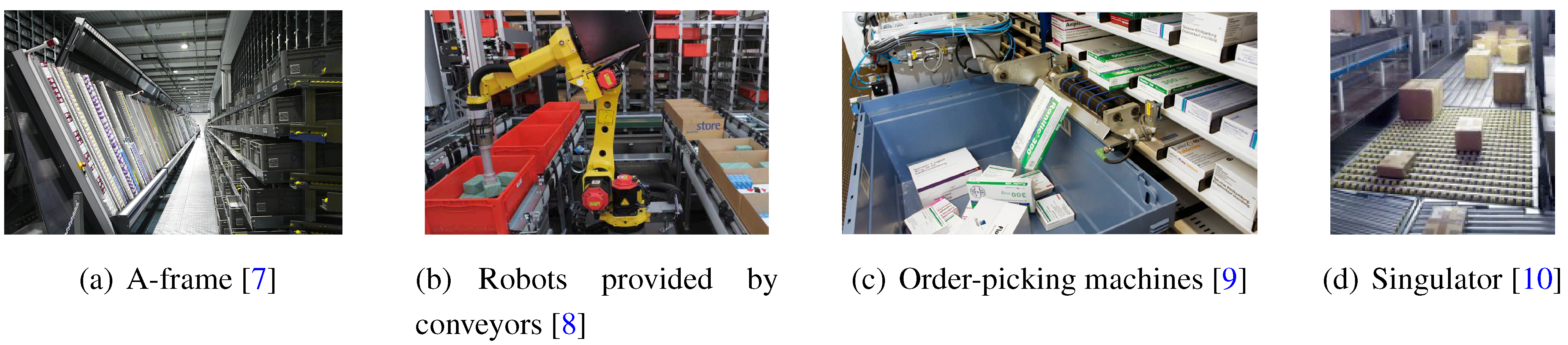
2.1. Fully Automated Order Picking

Distribution in commerce and industry is usually based on different trade levels. Along the supply chain—from producer to consumer—loading units are suspended and repacked. Large production lots are reallocated to smaller selling units. An important sub function for processes in facility logistics is the separation of piece goods. This so-called order picking is targeted by definition on assembling subsets out of an assortment due to requirements (customer order) [5]. Reaching this aim normally demands the separation of single goods out of bigger packaging units.

Manual separation processes are labor- and cost-intensive, so automated solutions could help to increase efficiency and reduce through-put time of orders at the same time. Contrary to these advantages, a huge number of factors impede the automated separation. First of all, complex and varying contours of the picking goods as well as a hardly predictable probability of quantity limit automated solutions for order picking to a defined spectrum of goods. Particularly block shaped packages and trays are well suited for machinable handling. Hence, shape, size, and quality of positioning have a crucial impact on the performance of automated order picking systems [6].

An example of known solutions for the automated order picking of small packages is shown in Figure 1. In these so-called A-frames, the goods are stored in vertical slots. According to costumer orders, they are separately ejected to a belt conveyor or into a bin. These systems stand out due to high performance but are limited to just a few packaging sizes and shapes.

Figure 1. Different solutions of automated order-picking.

Figure 1. Different solutions of automated order-picking.

Robots are also well aware in automated order-picking. As shown in Figure 1b, a gripper equipped robot singularizes goods out of bins. This solution allows high dynamics and flexibility. Depending on the processing time needed for the recognition of the gripping object and position, an adequate length of the supply belt is mandatory. Under certain conditions, this leads to large space requirements caused by long conveyor belts. Besides, these oder-picking machines (cf. Figure 1c) are used for special types of goods (e.g., pharmaceuticals), usually stored in large drug stores or dispensaries. In these cases, a small rack feeder reloads packages stored in shelves. Due to individual access to each storing object, high flexibility is a major advantage of this approach; however, due to the individual handling, the performance is rather low. A different approach is presented in Figure 1d. Karaca et al. [11] describe a calibrated multi camera vision system for real time tracking of parcels moving on a special conveyor belt. This belt consists of several independently controlled and moved sub-belts to arrange a bunch of parcels into a single line. Separated or singulated this way, the goods could be sorted mechanically to several chutes to complete an order. With a high throughput, this solution is suitable only for a limited spectrum of goods with a certain footprint and stiff package bottoms, i.e., they are unsuitable for pouches in general.

As already mentioned in Section 1, the automated separation of pouch packed goods is particularly challenging. They are usually stored in loose heaps or bins with no established order due to the difficult handling of limp goods. Beside the mentioned applications in Figure 1, some technical solutions are known for pouches. These solutions usually work with several belts or rollers in series, operating with different rotation speed to separate single packages from a heap (e.g., SpaceFeeder [12] or Automated Pouch Singulator [13]). Notably, these approaches have significant disadvantages concerning space requirements and they are not solving the complete picking task compared with the novel solution that this paper focuses on.

In principle, the picking system used in this paper may be deployed in any warehouse environemnt, regardless of whether the other logistical processes are done automatically or manually. However, to increase efficiency and reduce throughput times, it is intended to be integrated in a fully automated industrial environment. Moreover, the picking system can be cascaded using multiple machines to support the (automated) order-picking of different types of goods because a single machinery is only able to process one type of pouches at a time.

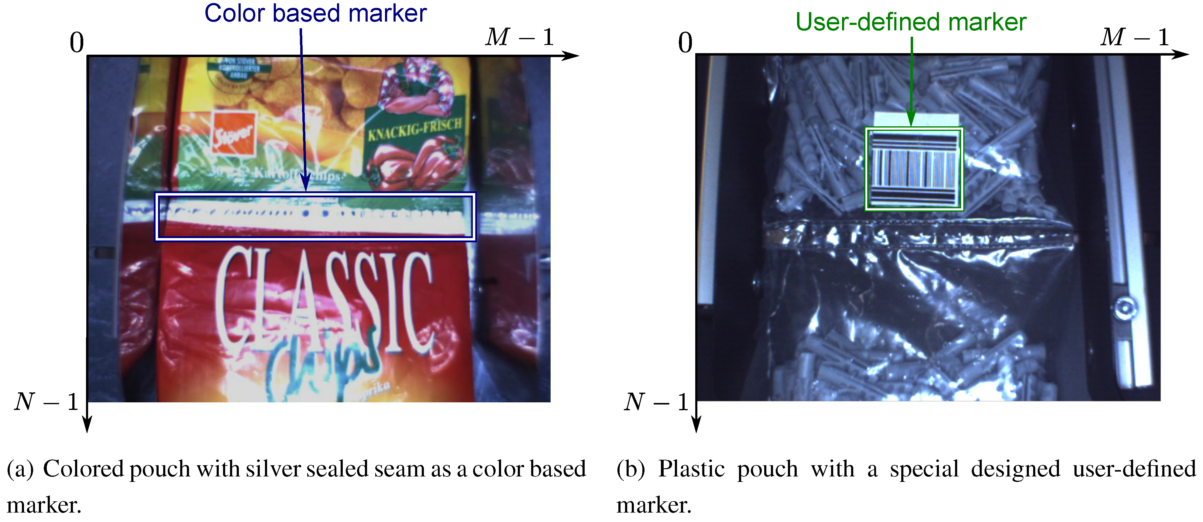
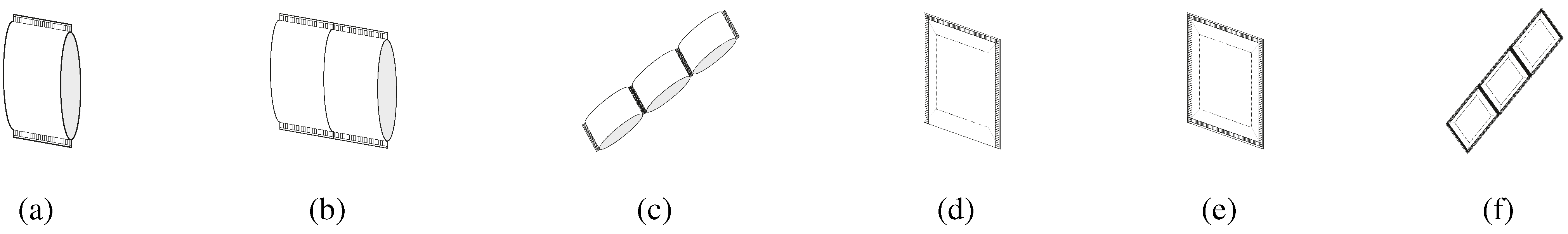
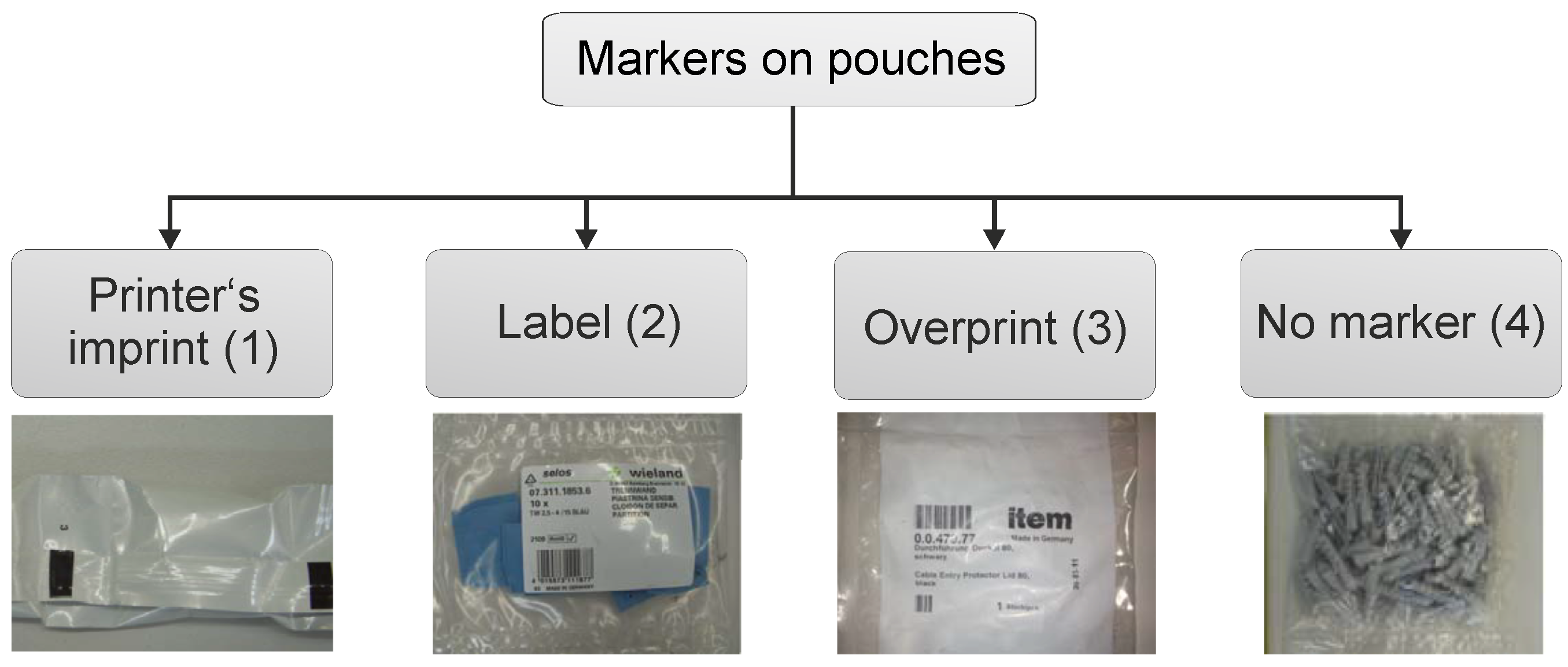
2.2. Types of Pouches in Industrial Systems

In this section, different types of pouches and their markers are presented which are usually used for packaging goods. They emphasize the variety and complexity of pouch packagings—Figure 2 gives an overview. Tubular pouches (see types (a) to (b) in Figure 2) are the most common pouches in the retail sector (especially food) and well suited to build chains. In most cases, a vertical bag forming, filling and sealing machine processes these pouches automatically. Usually, sealing the bottom of the pouch and cutting is one production step. By omitting the last step during the processing of each pouch, a defined chain accrues (e.g., type (c) in Figure 2).

Figure 2. Common shapes of flat pouches used for bag chains. (a,b) tubular pouches produced with or without side gussets; (c) a chain of tabular bags; (d) 3-side sealed bag; (e) 4-side sealed bag; (f) sealed seam bags as double or chain.

Figure 2. Common shapes of flat pouches used for bag chains. (a,b) tubular pouches produced with or without side gussets; (c) a chain of tabular bags; (d) 3-side sealed bag; (e) 4-side sealed bag; (f) sealed seam bags as double or chain.

Beside form and production method, different ways of marking the pouches and storing the needed information about their content are known in the industry. As shown in Figure 3, four general cases could be distinguished, depending on the production process of the pouches.

While using bag forming, filling and sealing machines in combination with graphics or pre-printed information on the foil, a printer’s imprint (also called registration mark) is mandatory to detect the accurate placement of the pouches. Printing process variations, film stretch, film slippage during acceleration and other factors can allow the graphics to drift away from ideal cosmetic/marketing placement on the finished bag. The registration mark provides a method to make minor adjustments to the actual end placement of the seal and cut on a bag [15]. An example for a printer’s imprint or registration mark is given on the left side (1) of Figure 3. In some cases, the vertical seam may cover the registration mark after producing the pouch where the longitudinal sides of the flat foil are welded to a tubular shape. Otherwise, printer imprints are suitable for post-production cutting line detection. When there is no printing or graphics on the bag, the production process is defined solely on length (cf. right side of Figure 3). This type of pouches usually gets a label or overprint (see (2) and (3) in Figure 3) during or after production to identify the content (e.g., a bar code). While these markers are attached during the packaging process, they could also be used for post-production cutting line detection. However, the proposed method will not work for uniformly designed pouches without any recognizable mark.

Figure 3. Systematic of possible different ways to mark a pouch.

Figure 3. Systematic of possible different ways to mark a pouch.

2.3. Cutting Line Detection

Different options concerning detection of sealed seams are presented within this section. Today’s systems of cutting line detection are based on the recognition of printer’s imprint placed on the packaging material. Efficient working sensors are well available on the market, usually deployed in print and packaging applications. Four different types could be distinguished [16]:

• binary registration (print) mark sensor based on contrast or color (e.g., SICK KT 10-2),
• binary camera based sensors,
• camera systems (e.g., SICK IVC-2D or IVC 3D),
• and sensors for detection of streams of marks.

High sensitivity against changing distances between the sensor and the detected goods is the main drawback of the mentioned technologies. Usually, so-called registration mark sensors (e.g., SICK AX20) work with a detection distance of 10 to 50 mm; the tolerance against distance changes is even less. Inherent to the presented order picking system for pouches, the distance between the detection unit and the chain of pouches is not constant. This is caused by type and orientation of the goods inside the pouch. Given these undefined outlines, the pouches vary in length and depth which virtually prevents the use of the listed sensor technologies except for 2D- and 3D- camera systems.

However, compared to standard sensors, the use of commercially available 2D or 3D vision systems for the detection causes high costs. Hence, a flexible, low cost and robust concept has to be developed which enables the detection of various sealed seams. Instead of dedicated sensors, a combination of a CCD camera, an off-the-shelf desktop PC and a detection algorithm is used. By surrendering specialized solutions like “Smart Cameras”, cost efficiency is granted.

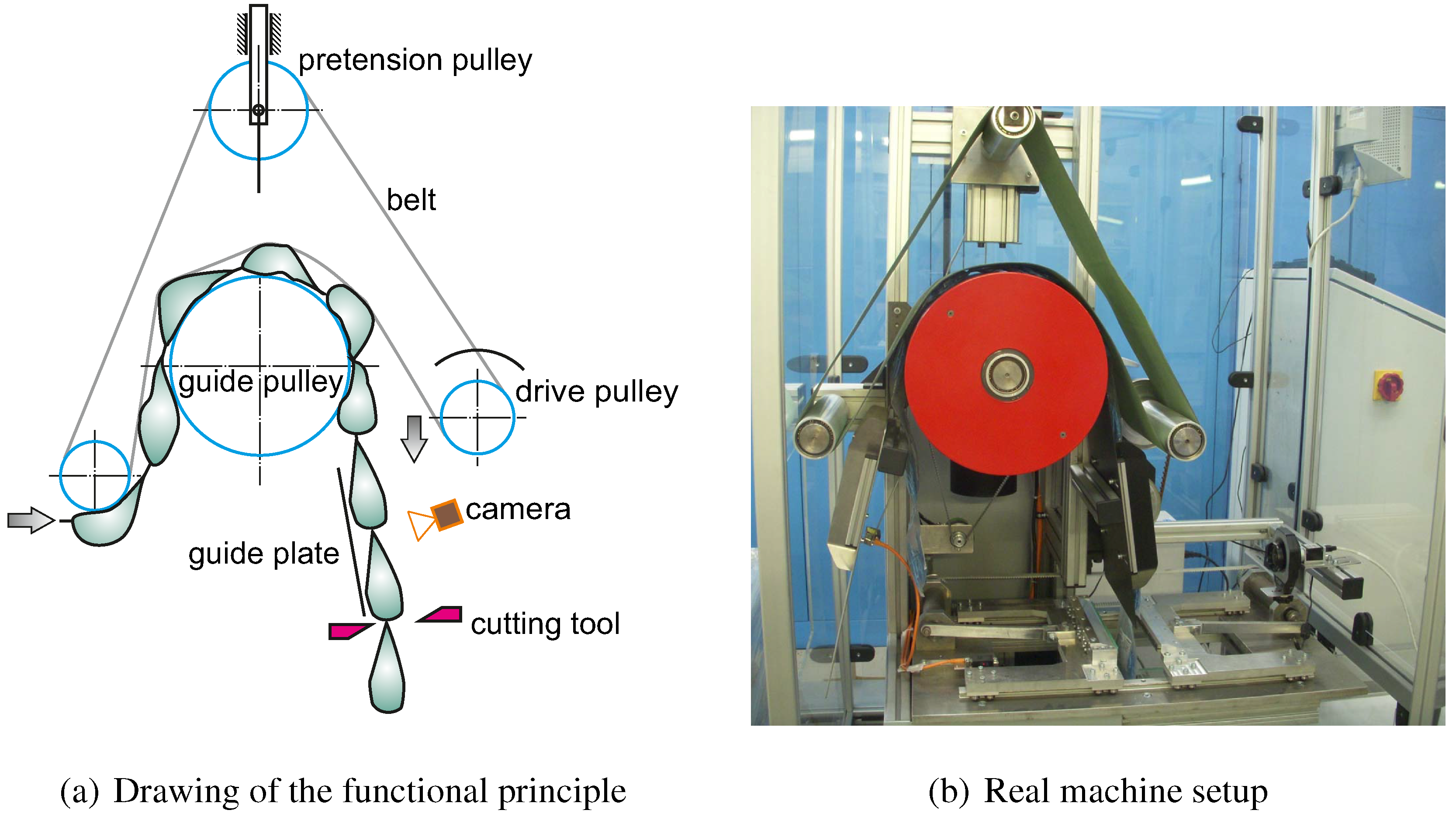
3. Automated Order Picking System

Within this section, the details of the automated order picking system are presented. It is built up of three components: the mechanical, the control and the vision component. Details of the mechanical setup and the intercommunication by the control system are explained in this section while the vision system is detailed in Section 5.1.

In Figure 4a, a drawing of the functional principle is shown. The real setup is depicted in Figure 4b which shows the mechanical setup (left) and the vision system (right). A dispensing mechanism based on a modified cover band principle is responsible for feeding the pouch chain through the system. Powered by a drive pulley, the belt covers the goods which roll over the guide pulley. Slack-side tension of the belt is imposed and maintained at a constant level by a floating tension pulley which compensates for belt elongation and changes in the thickness of the pouch chain inside the machine. Thus, the friction between the cover belt and the pouch chain advances the goods [3]. An incremental position encoder compares the number of revolutions of the guide pulley with the number of revolutions of the drive pulley in order to tentatively ensure a constant velocity level. The integrated cutting unit consists of two parallel linear blades and a servo eccentric drive which allows up to 4 cuts per seconds. All sensors and actuators are controlled by a soft Programmable Logic Controller (PLC) located on an external computer.

Figure 4. Drawing of the functional principle and the needed components (a) and the real setup at the Fraunhofer Institute for Material Flow and Logistics (b).

Figure 4. Drawing of the functional principle and the needed components (a) and the real setup at the Fraunhofer Institute for Material Flow and Logistics (b).

The picking process is started by the inquiry of the required number of pouches. A specific marker profile attached to each of the pouches enables the vision system to detect the cutting line. In Figure 5, two different approaches for the interaction of the sensor (CCD camera) and the actuators (servo drive and cutting tool) are presented. Depending on these approaches, the controlling strategies differ, too. They specify how the marker detection module (blue, dashed) interacts with the machine control (gray). On the one hand, a clocked solution (see Figure 5a) may be realized. In this case, a defined feed (roughly having the length of a single pouch) is processed by the PLC. A position request from the PLC opens a control loop that sends back the actual position of the detected marker. If the marker is detected in a possible cutting position, one or more pouches can be separated. Otherwise, a correction of the position has to be executed before a new request is accomplished by the PLC. This process will be repeated until the desired number of pouches is separated. In terms of time, this implementation is not critical since the processed images only show static pouch chains.

Figure 5. Interaction of the sensor (red) and actuators (green) in terms of two controlling strategies of the picking system: (a) clocked and (b) “on the fly” mode of operation. Figure 8 depicts the details of the “marker detection” module (dashed) which are presented throughout this paper. It serves as the (algorithmic) interface between the sensor and actuators.

Figure 5. Interaction of the sensor (red) and actuators (green) in terms of two controlling strategies of the picking system: (a) clocked and (b) “on the fly” mode of operation. Figure 8 depicts the details of the “marker detection” module (dashed) which are presented throughout this paper. It serves as the (algorithmic) interface between the sensor and actuators.

Another solution is based on a continuous “on the fly” principle (see Figure 5b). In this case, marker detection is processed permanently analog to the cover belt traction. As far as a marker is detected in cutting position, the cutting command is immediately send to the PLC. When the number of ordered pouches has been reached, the drive of the cover belt stops. Literally, the latter control approach convinces with simplicity since only three commands are required; however, apart from that it is time-sensitive. Depending on conveying speed, pouch length, and marker size, the overall processing time has to be lower than the feed duration between two markers. For the sake of throughput, the marker detection algorithms presented in this paper are solely based on the continuous “on the fly” principle.

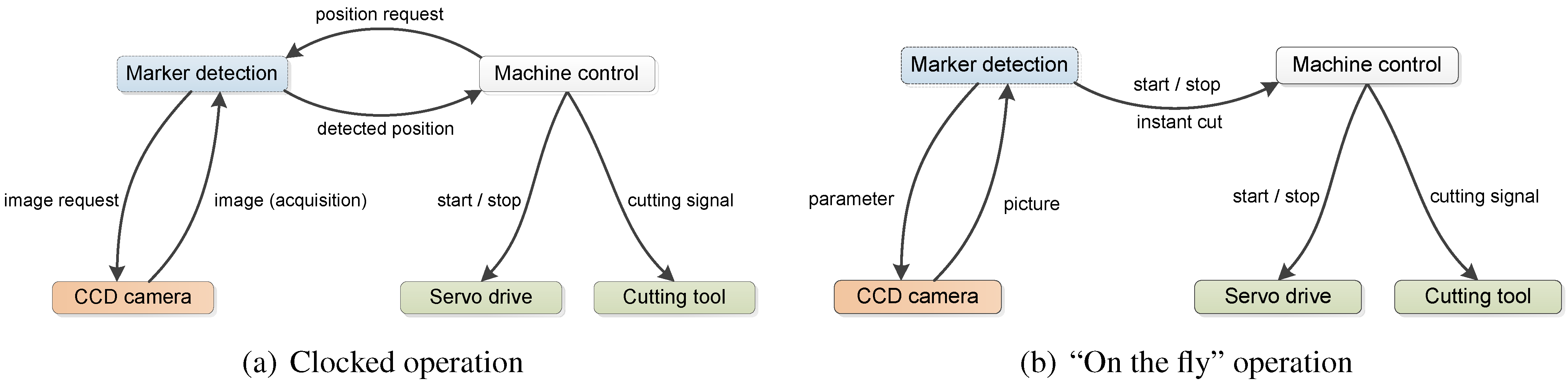
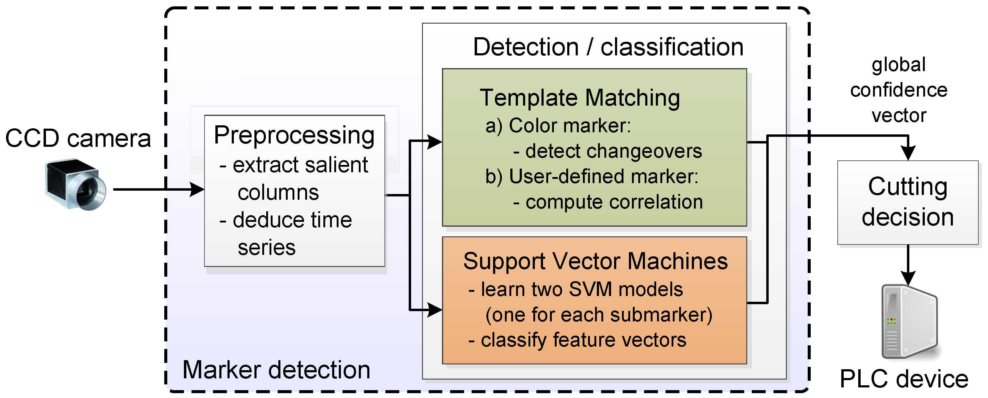
4. Marker Detection System

Given the setup described in the previous section, a CCD camera observes the ongoing pouches (cf. Figure 4). The attached marker on each pouch enables the vision component to detect whether a pouch is currently in cutting position. The images are provided by an industrial camera and the processing is executed on a desktop PC allowing an overall robust and low-cost solution.

The markers and the appropriate detection algorithms are described in the next sections.

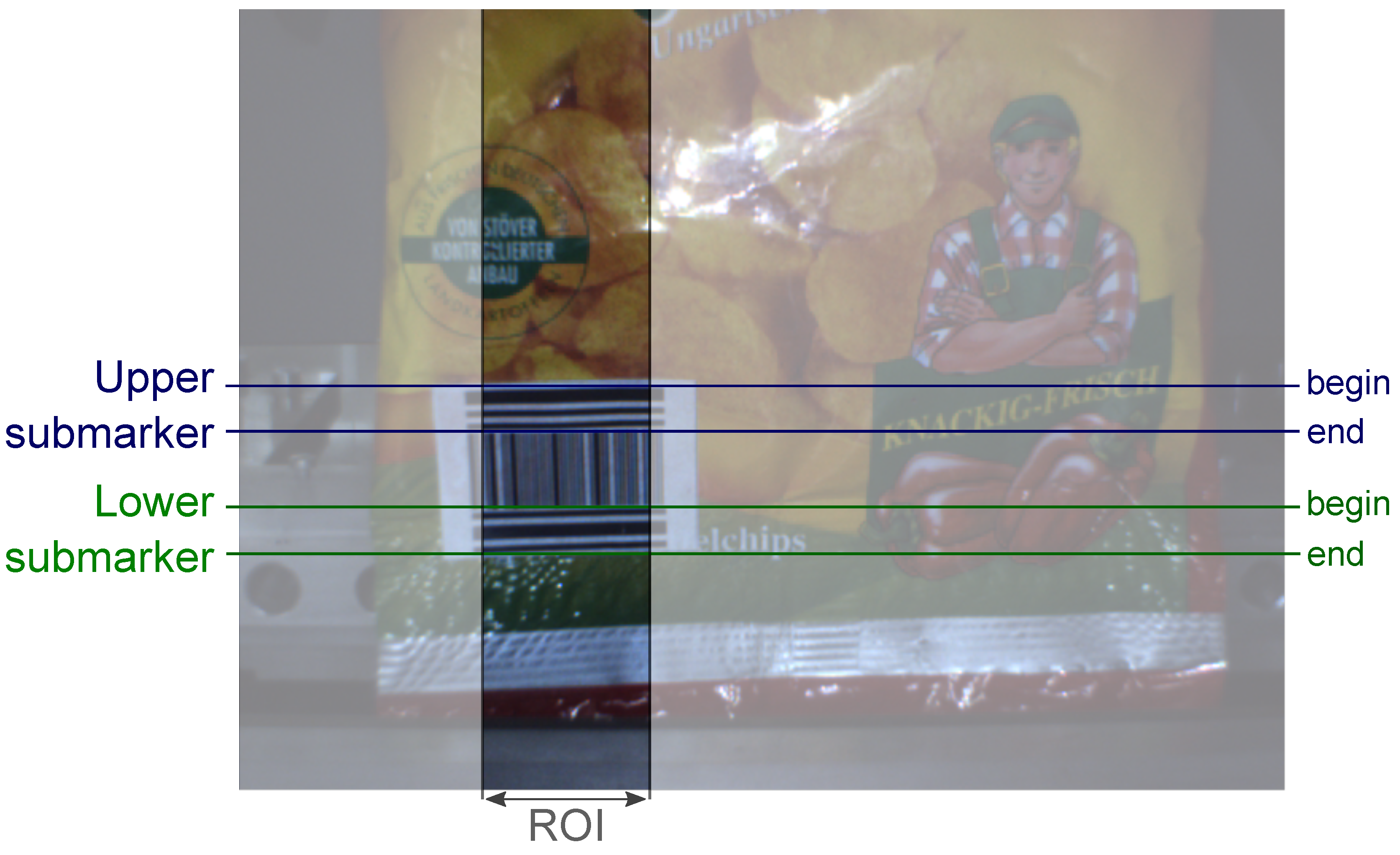
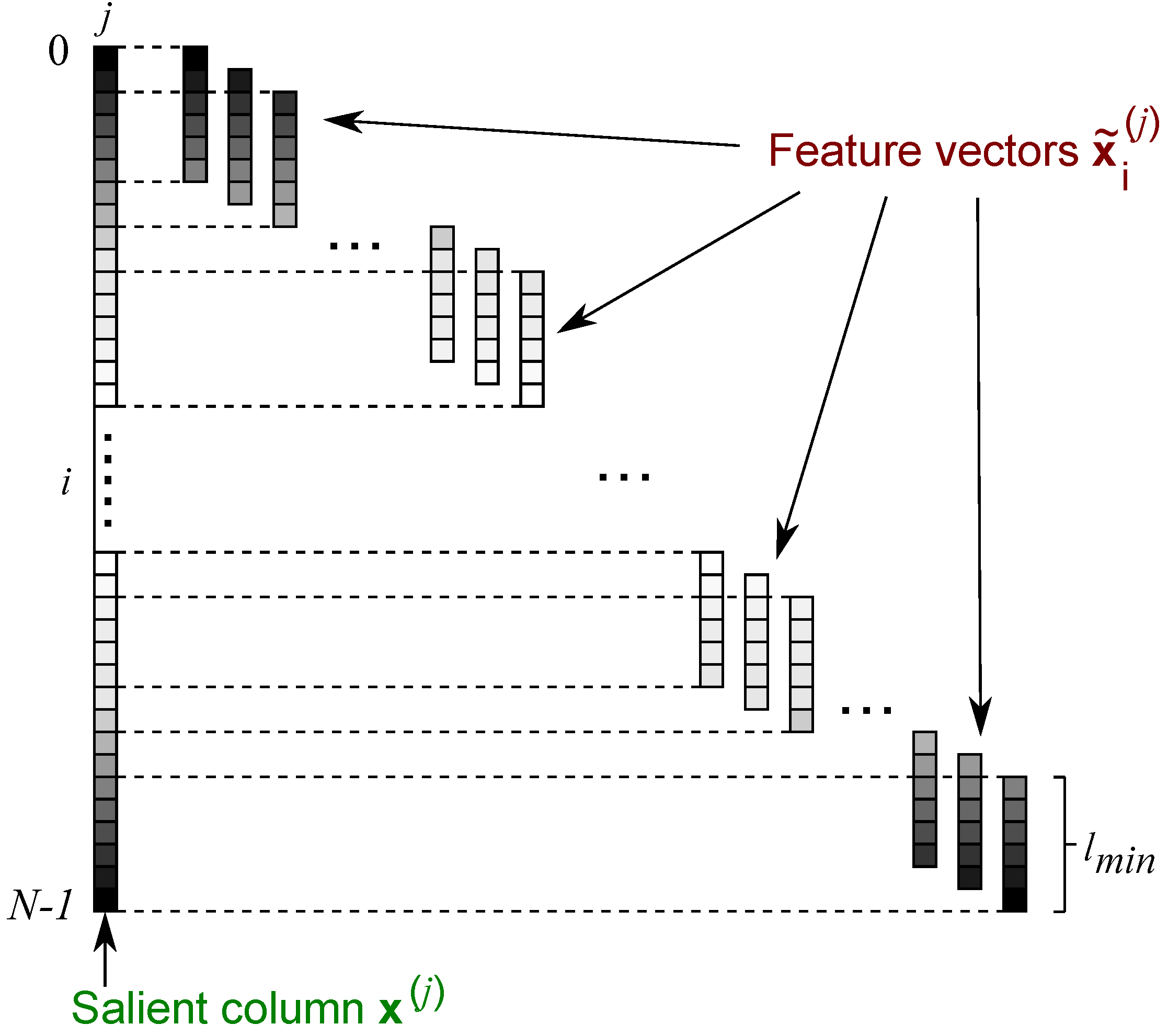
4.1. Marker Detection

The marker detection algorithms support two types of markers, a color based marker and a specially designed “user-defined marker” as visualized in Figure 6. The detection of the color based marker is performed with a histogram enhanced template matching (Color-Marker_Template) whereas in addition to a template-based approach (UD-Marker_Template), a machine learning concept (UD-Marker_SVM) is used for the detection of the user-defined (UD) marker. This section introduces the marker detection concepts from a methodical point of view: Color-Marker_Template and UD-Marker_Template as heuristic concepts and UD-Marker_SVM as a supervised classification based concept.

Figure 6. Two different types of marker: (a) a silver sealed seam as a color based marker and (b) a plastic pouch with a specially designed user-defined marker.

Figure 6. Two different types of marker: (a) a silver sealed seam as a color based marker and (b) a plastic pouch with a specially designed user-defined marker.

Figure 7. Schematic concept of the (Left) extraction of $k\le M$ salient columns ${}^{\rho }{\mathbf{x}}^{(j)}=\{{}^{\rho }{x}_0^{(j)},\dots ,{}^{\rho }{x}_i^{(j)},\dots ,{}^{\rho }{x}_{N-1}^{(j)}\}$ from an image of size $N\times M$ pixels–the RGB-channel is represented by $\rho \in \{r,g,b\}$. The salient columns undergo a classification process leading to a time series which assigns the image rows a specific probability of containing the marker (Right).

Figure 7. Schematic concept of the (Left) extraction of $k\le M$ salient columns ${}^{\rho }{\mathbf{x}}^{(j)}=\{{}^{\rho }{x}_0^{(j)},\dots ,{}^{\rho }{x}_i^{(j)},\dots ,{}^{\rho }{x}_{N-1}^{(j)}\}$ from an image of size $N\times M$ pixels–the RGB-channel is represented by $\rho \in \{r,g,b\}$. The salient columns undergo a classification process leading to a time series which assigns the image rows a specific probability of containing the marker (Right).

The key idea of both concepts is the representation of an image column j as time series ${}^{\rho }{\mathbf{x}}^{(j)}=\{{}^{\rho }{x}_0^{(j)},\dots ,{}^{\rho }{x}_i^{(j)},\dots ,{}^{\rho }{x}_{N-1}^{(j)}\}$ while each image line i represents a discrete time step with a specified probability (in the following equivalent to the notation confidence) of containing the marker as visualized in Figure 7. $\rho \in \{r,g,b\}$ denotes the RGB channel of the input image. The two concepts differ in the way of deducing the time series which are finally analyzed in order to detect the marker.

The detection algorithm is applied on the images, provided by the camera, and consists of several substeps as shown in Figure 8. In the preprocessing step, a set of salient columns is extracted followed by deducing time series of the selected image columns. Then the deduced time series undergoes a detection/classification (Color-Marker_Template, UD-Marker_SVM and UD-Marker_Template) producing a confidence vector for each time series. Finally, the confidence vectors are combined to a global confidence vector which serves as the input for the decision-finding in order to detect the marker.

Figure 8. Pipeline of the vision based marker detection system (dashed boxes in Figure 5). The classification step of the color based marker detection proceeds with Template Matching while the user-defined marker is detected by supervised classification (SVMs).

Figure 8. Pipeline of the vision based marker detection system (dashed boxes in Figure 5). The classification step of the color based marker detection proceeds with Template Matching while the user-defined marker is detected by supervised classification (SVMs).

4.2. Color Marker Detection

The model of the color based marker consists of a color component and the vertical dimension ${\theta }_v$ of the marker as shown in Figure 9. The color component is deduced by constructing a three-dimensional histogram of the image pixel intensity values of the RGB channels. The histogram space is equidistantly subdivided into quads which are analyzed with respect to their density. Figure 9b exemplary visualizes a three-dimensional histogram. Each sphere represents one sub quad while the size of the sphere symbolizes the count of the pixels in the sub quad . All intensities of the marker lie in the region of the marked sphere which represents the sub quad ${\sigma }_v$. Beside the marker pixels, additional pixels from image regions with light reflections fall in this region. Hence, a pure intensity based classification is insufficient. Therefore, an additional feature is needed for an explicit representation of the marker. In this context, the vertical dimension ${\theta }_v$ of the marker is taken into account as illustrated in Figure 9a.

Figure 9. Model of the color based marker depending on the (a) vertical image dimension ${\theta }_v$ of the marker and (b) the three dimensional RGB histogram. The size of the spheres symbolizes the pixel count in the subquads.

Figure 9. Model of the color based marker depending on the (a) vertical image dimension ${\theta }_v$ of the marker and (b) the three dimensional RGB histogram. The size of the spheres symbolizes the pixel count in the subquads.

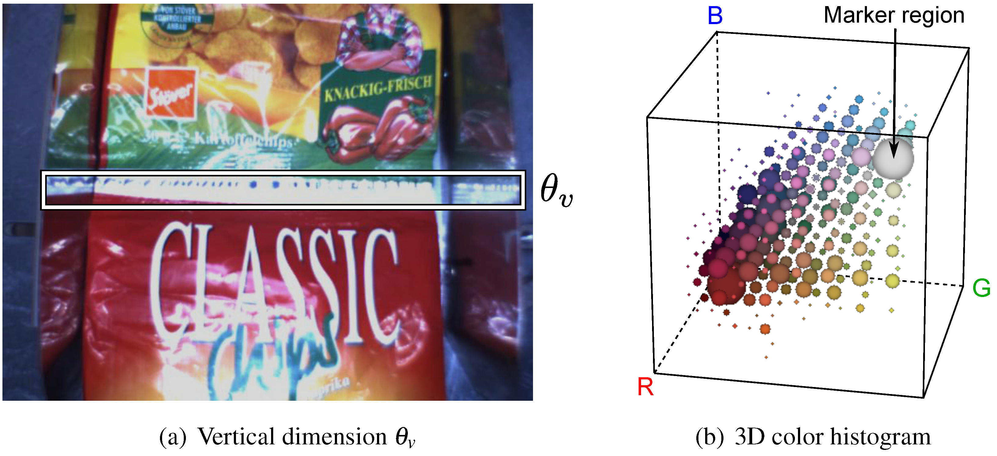
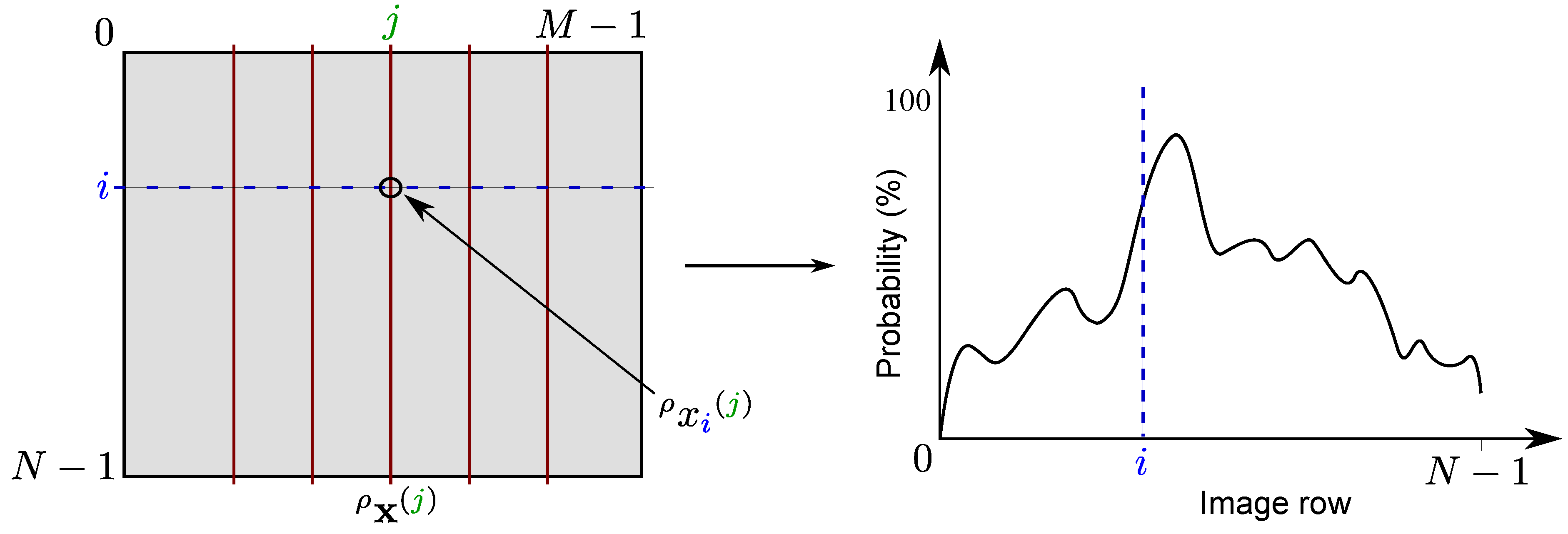
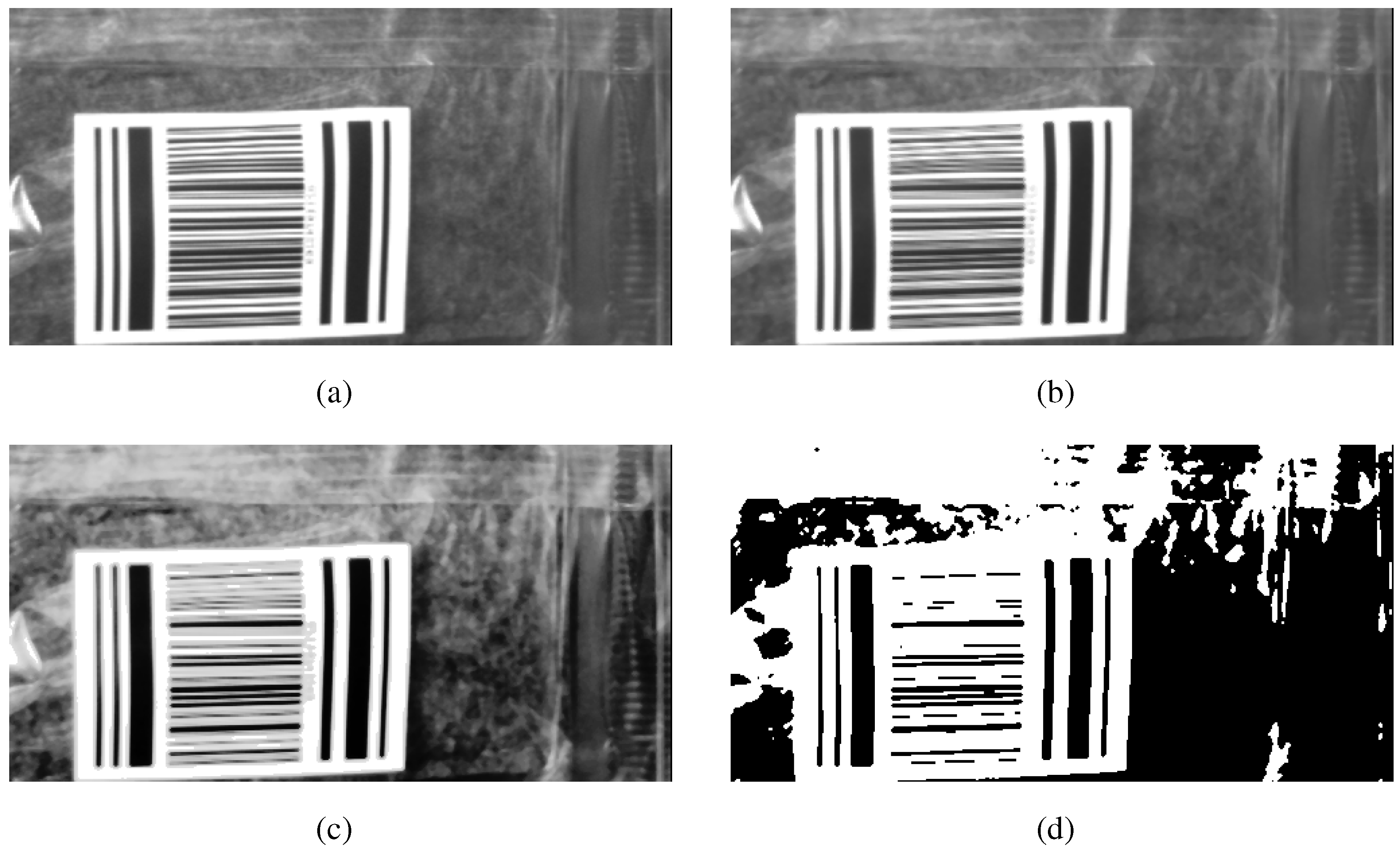
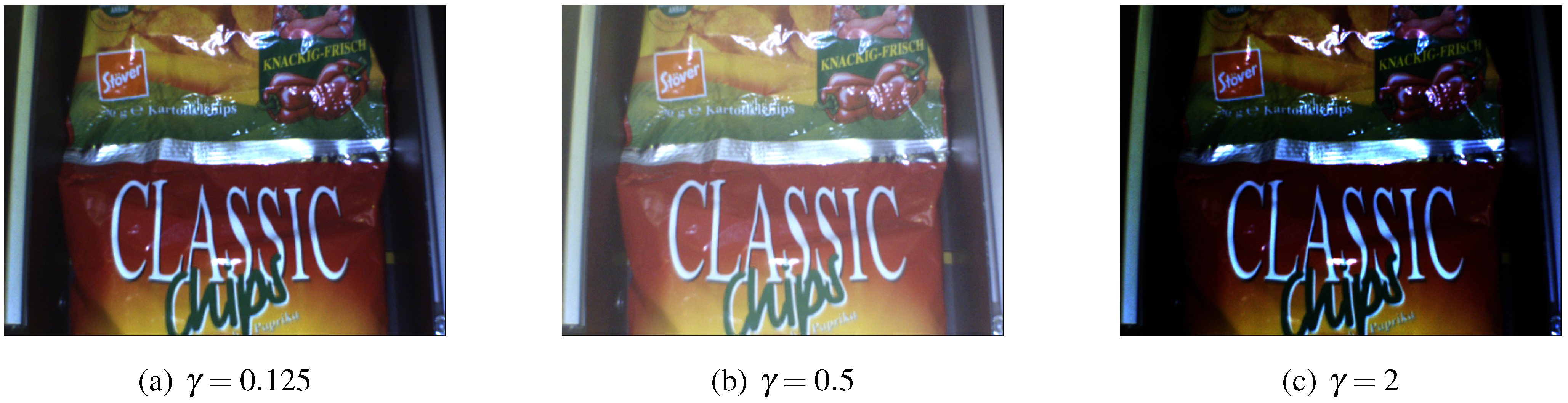
4.2.1. Preprocessing

In order to equalize different illumination conditions, the contrast of the image is enhanced by the help of histogram equalization. Therefore the RGB image is converted to the YUV format first, followed by a histogram equalization of the Y channel. Finally, the enhanced YUV image is converted back to the RGB format. In the next step, salient columns are extracted from the image.

The extraction set $\mathcal{X}\in \{{}^{\rho }{\mathbf{x}}^{(0)},\dots ,{}^{\rho }{\mathbf{x}}^{(j)},\dots ,{}^{\rho }{\mathbf{x}}^{(k-1)}\}$ of the $k=\left|\mathcal{X}\right|\le M$ salient columns ${}^{\rho }{\mathbf{x}}^{(j)}=\{{}^{\rho }{x}_0^{(j)},\dots ,{}^{\rho }{x}_i^{(j)},\dots ,{}^{\rho }{x}_{N-1}^{(j)}\}$ is based on the object model which consists of a color component and the vertical dimension ${\theta }_v$ of the marker. In terms of reducing the calculation time, extracting few salient image columns is a remedy, keeping in mind the trade-off between detection quality and calculation time. The selected image columns are analyzed in further pipeline steps.

The extracted salient columns are represented as intensity vectors for each RGB channel ρ while the image lines serve as time steps. Hence, for each salient column ${\mathbf{x}}^{(j)}$ we get three vectors ${}^r{\mathbf{x}}^{(j)}$, ${}^g{\mathbf{x}}^{(j)}$, ${}^b{\mathbf{x}}^{(j)}$ as time series.

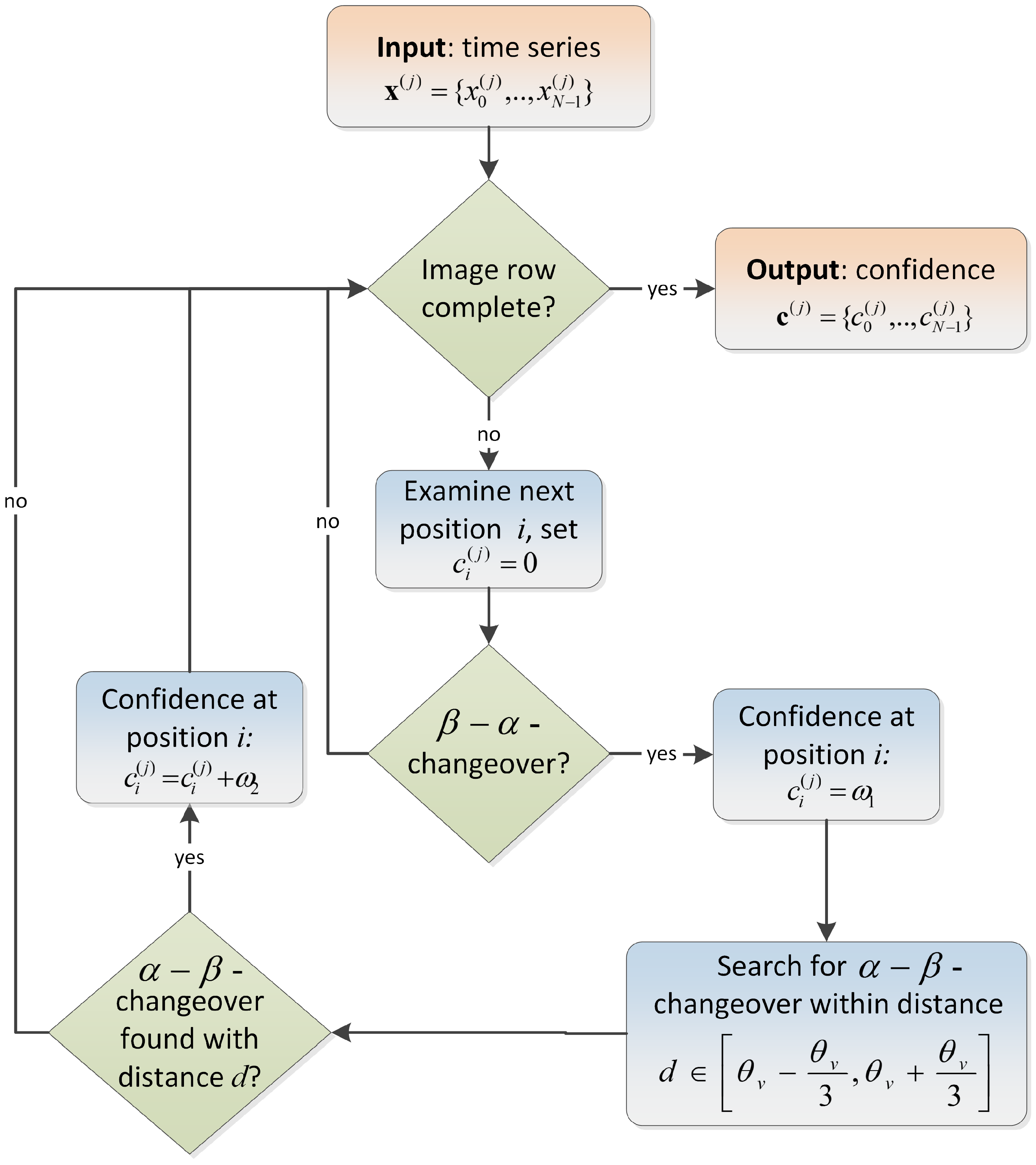
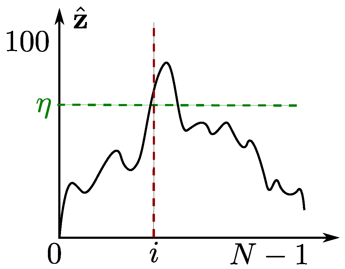
4.2.2. Histogram-Enhanced Template Matching (Color-Marker_Template)

Based on the deduced time series of the salient image columns, for each time step (which represents a particular image row) a correlation is calculated resulting in a confidence vector which indicates the probability of containing the marker. The process of constructing the confidence vector is illustrated in Figure 10 and described in detail in the following. First, the histogram based classification is examined which segments the pixels (time steps of the time series) into potentially marker candidates α and the rest β. Let σ define the subspace in the three dimensional RGB histogram which represents the marker pixel values. A pixel $x_i^{(j)}$ is assigned to potential marker candidate, if the RGB values of $x_i^{(j)}$ fall in the RGB subspace σ:

• ${\alpha }_r\in {\sigma }_{r_1,r_2}^r,r_1,r_2\in \mathbb{N},r_1,r_2\le 255,r_1\le r_2$: ${\sigma }_{r_1,r_2}^r$ interval which contains the red channel intensity values ${\alpha }_r$ of the subquad.
• ${\alpha }_g\in {\sigma }_{g_1,g_2}^g,g_1,g_2\in \mathbb{N},g_1,g_2\le 255,g_1\le g_2$: ${\sigma }_{g_1,g_2}^g$ interval which contains the green channel intensity values ${\alpha }_g$ of the subquad.
• ${\alpha }_b\in {\sigma }_{b_1,b_2}^b,b_1,b_2\in \mathbb{N},b_1,b_2\le 255,b_1\le b_2$: ${\sigma }_{b_1,b_2}^b$ interval which contains the blue channel intensity values ${\alpha }_b$ of the subquad.

Otherwise pixel $x_i^{(j)}$ is assigned to β. After that, each pixel of the salient columns is mapped either to α or to β.

Figure 10. Flow chart for constructing confidence vectors ${\mathbf{c}}^{(j)}$ for a particular time series ${\mathbf{x}}^{(j)}$. Input and output is visualized in Figure 11a,c. α represents predefined marker candidate pixels based on the RGB color model and β represents pixels from the rest of the image.

Figure 10. Flow chart for constructing confidence vectors ${\mathbf{c}}^{(j)}$ for a particular time series ${\mathbf{x}}^{(j)}$. Input and output is visualized in Figure 11a,c. α represents predefined marker candidate pixels based on the RGB color model and β represents pixels from the rest of the image.

The histogram based classification is used to construct a confidence vector ${\mathbf{c}}^{(j)}=\{c_0^{(j)},\dots ,c_i^{(j)},\dots ,c_{N-1}^{(j)}\}$ for each time series ${\mathbf{x}}^{(j)}$ which uses the vertical dimension $\theta \in \mathbb{N}$ of the marker and detects $\beta -\alpha$ (no marker → marker) and $\alpha -\beta$- (marker → no marker) changeovers. In terms of robustness, a changeover is detected when s β-pixels follow directly after s α-pixels ($s\in \mathbb{N}$, $s\ge 1$). The search for a marker begins with a $\beta -\alpha$- (no marker → marker) changeover and ends with a $\alpha -\beta$- (marker → no marker) changeover. For a time series ${\mathbf{x}}^{(j)}$, if a $\alpha -\beta$-changeover is found at position i, the confidence vector stores the confidence value ${\omega }_1$ at position i as $c_i^{(j)}={\omega }_1$, whereby ${\omega }_1\in \mathbb{N}$ is an arbitrary constant. After finding the start position i of the marker, the search for the end position of the marker is performed with a sliding window of a defined size. In an ideal constellation, the sliding window has the size of the vertical dimension of the marker ${\theta }_v$ (cf. Figure 11a).

Figure 11. Classification of time series ${\mathbf{x}}^{(j)}$ of a synthetic image shown in (a) to marker candidates ($\alpha \in \mathbb{N}$) and no marker time steps ($\beta =0$). The subsequent process of constructing a confidence vector ${\mathbf{c}}^{(j)}$ based on (b) is depicted in (c).

Figure 11. Classification of time series ${\mathbf{x}}^{(j)}$ of a synthetic image shown in (a) to marker candidates ($\alpha \in \mathbb{N}$) and no marker time steps ($\beta =0$). The subsequent process of constructing a confidence vector ${\mathbf{c}}^{(j)}$ based on (b) is depicted in (c).

Considering the vertical marker dimension ${\theta }_v$ and, e. g., the fact that the marker is not perfectly horizontally aligned to the image lines due to irregular materials and buckling, a tolerance interval $[{\theta }_v-\frac{{\theta }_v}{3},{\theta }_v+\frac{{\theta }_v}{3}]$ is used as the size of the sliding window. Therefore, if a $\alpha -\beta$-changeover is found within distance $d\in [{\theta }_v-\frac{{\theta }_v}{3},{\theta }_v+\frac{{\theta }_v}{3}]$ after a $\beta -\alpha$-changeover followed by α- (marker) candidates, the confidence (founding a marker at position i) increases to $c_i^{(j)}=c_i^{(j)}+{\omega }_2$, whereby ${\omega }_2\in \mathbb{N}$ is an arbitrary constant, too. Figure 10 visualizes the process of constructing the confidence vector by exemplary assigning a confidence to a particular pixel (time step) of a salient image column (time series).

The result of the Color-Marker_Template are $k\le M$ confidence vectors ${\mathbf{c}}^{(0)},\dots ,$ ${\mathbf{c}}^{(j)},\dots ,$ ${\mathbf{c}}^{(k-1)}$ constructed from k time series (salient columns). The domain of each confidence vector consists of three different types of values, namely 0, ${\omega }_1$ or ${\omega }_1+{\omega }_2$, with $0\le {\omega }_1\le {\omega }_1+{\omega }_2$. While ${\omega }_1+{\omega }_2$ represents a high probability to include a marker at the corresponding time step (pixel), ${\omega }_1$ is a weaker indication and other values are remarked with 0.

In the next step, unique confidence vectors are combined into a global confidence vector $\mathbf{z}=\{z_0,\dots ,z_i,\dots ,z_{N-1}\}$. The global confidence vector is built as a sum of the particular confidence vectors:

$$z_i=\sum _{j=0}^{k-1}{c}_i^{(j)},k\le M.$$

(1)

In terms of optimization, $z_i$ is smoothed with a window operator with the window size $\delta \in \mathbb{N}$ which is empirically determined:

$$\widehat{z_i}=\sum _{w=-\frac{\delta }{2}}^{\frac{\delta }{2}}{z}_{i+w}.$$

(2)

Finally, a search for the maximum ${\widehat{z}}_{max}$ of $\widehat{z_i}$ is performed. An empirically user-defined bound $\eta \in \mathbb{N}$ builds an additional demand on the found marker position. Hence, ${\widehat{z}}_{max}$ represents a marker position if ${\widehat{z}}_{max}>\eta$ as illustrated in Figure 12.

Figure 12. Detected marker position i with ${\widehat{z}}_i\ge \eta$ in the global confidence vector $\widehat{\mathbf{z}}$.

Figure 12. Detected marker position i with ${\widehat{z}}_i\ge \eta$ in the global confidence vector $\widehat{\mathbf{z}}$.

The template matching approach affords excellent results for special cases like the detection of the characteristic silver sealed seam of colored pouches as presented in the evaluation results in Section 5. Nevertheless, this concept leads to the disadvantage of manually defining the marker model for each type of pouch. The next section presents a learning based classification method which simplifies the adaption to new pouch types.

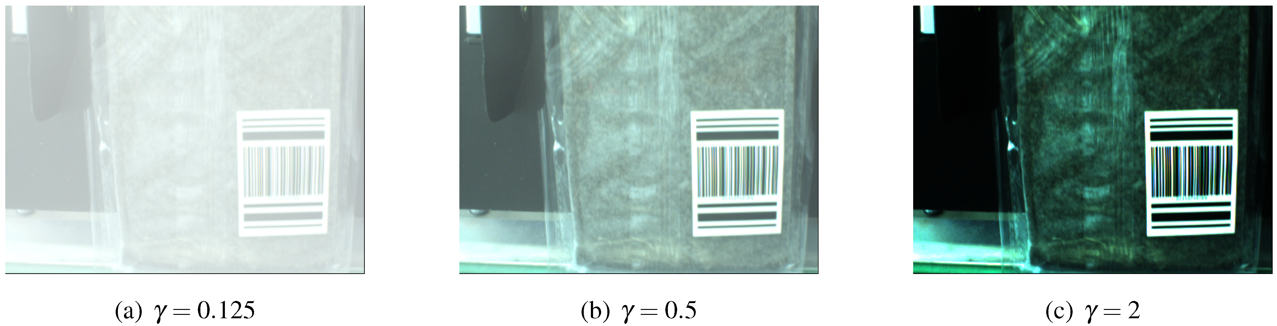
4.3. User-Defined Marker Detection

In this section, two approaches (UD-Marker_SVM and UD-Marker_Template) to detect user-defined (UD-) markers will be introduced. The use of one- or two-dimensional barcodes (like QR codes) was tested as well. Unfortunately, motion blur and varying distances between the camera and the pouches led to low detection rates making barcodes unsuitable in this context. Thus, the use of a user-defined marker is proposed which extents a typical barcode (located in between the user-defined submarkers). This way, logistic processes are still able to employ barcode technologies for identification purposes.

The first approach—described in Section 4.3.2—applies a machine learning method while the second approach (cf. Section 4.3.3) finds a user-defined marker by means of template matching. The main advance of machine learning (supervised classification) is not only the flexible portability to new marker and pouch types but also the robustness towards environmental changes as varying light conditions and artifacts. In the given case, Support Vector Machines (SVMs) assign objects to defined classes based on a learned classification model. For details of Support Vector Machines, see, e.g., [17,18]. In combination with the UD-Marker_SVM approach, an optimal marker was developed as visualized in Figure 13a and described in the following.

4.3.1. User-Defined Marker Design

Figure 13a visualizes the user-defined marker, designed for the UD-Marker_SVM approach. The special feature of the marker design is the integration of a barcode which is standard in industrial labeling. The new marker consists of two submarkers (with distance $d_2$) enclosing the barcode: the upper marker and lower submarker. The submarkers are built up of three vertical black bars, two bars of the same thickness and one twice thick as the other two. Between the bars, a constant distance $d_1$ is set which is a relevant value for the detection process as described in the evaluation (cf. Section 5.2.2). The upper and lower submarker differ in the alignment of the particular bars. The key idea (cf. Section 4.1) of the design of the marker is to represent the image as time series while each column specifies one time series and the image lines serve as particular time steps. Deducing one image column of the marker (ignoring the middle bar code) as time series of the intensity values, leads to a characteristic function as visualized on the right side of Figure 13b. For simplicity, the distance $d_{cut}$ between the marker and the optimal cutting line is assumed to be constant because $d(cut)$ is usually rather small compared to the size of the sealed seams so that the deformations of the pouches are negligible.

Figure 13. The design of the marker (a) approves deducing characteristic intensity profiles (b) of each image column (vertical red line in (a)) of the marker by analyzing the intensity values. The marker is integrated into the bar code (vertical bars) which does not take influence on the detection of the submarkes (horizontal bars).

Figure 13. The design of the marker (a) approves deducing characteristic intensity profiles (b) of each image column (vertical red line in (a)) of the marker by analyzing the intensity values. The marker is integrated into the bar code (vertical bars) which does not take influence on the detection of the submarkes (horizontal bars).

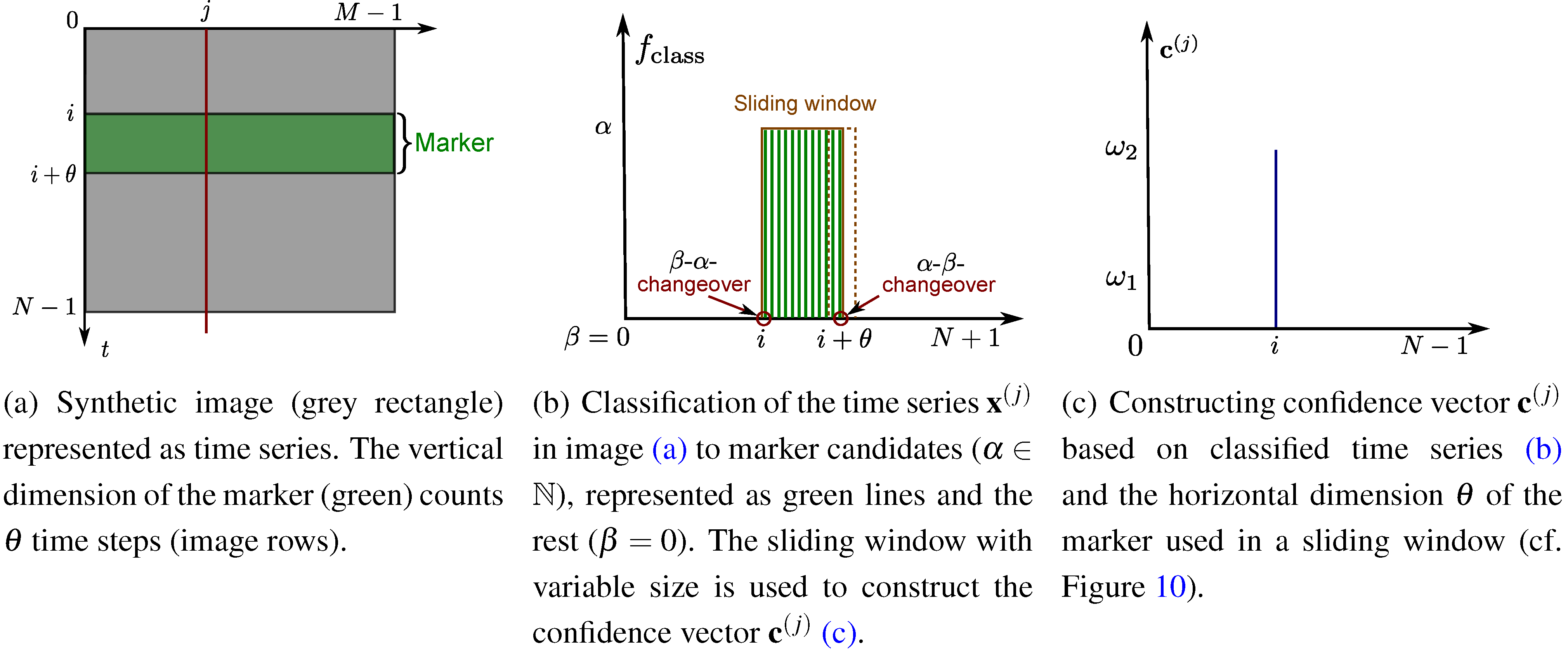
4.3.2. Machine Learning Based Marker Detection

The following paragraphs describe the machine learning based marker detection pipeline for the user-defined marker (UD-Marker_SVM). First of all, the SVM classification model is learned based on a representative set of exemplary images as described in the next paragraph. Once the SVM model is built, the current image is analyzed by extracting feature vectors from the image and classifying them by the SVM model in order to search for a marker. Then a confidence vector is built which represents the probability of containing the marker in each image line. Based on the confidence vector, a model for decision-finding is determined.

Preprocessing: 

In the first step, a Region of Interest (ROI) is defined which includes the marker as illustrated in Figure 14. Here, attention should be paid that the marker significantly differs from the rest of the ROI region. Because of the static setup (cf. Section 5.1), the marker is always found in the ROI. Image regions outside the ROI are not considered in the marker detection process; hence, excluding these regions decreases the calculation time. A set of images is captured which show the pouches with the marker in different positions. Because of irregular buckling of the pouches, the marker differs in position and rotation. For each image, the user manually marks two image regions, one including the upper and one representing the lower submarker as visualized in Figure 14. In terms of the marker detection process, two SVMs are learned separately, one for the upper and one for the lower submarker. Thus, two datasets are generated for the learning process, one for each of the two SVMs.

Figure 14. Definition of the Region of Interest (ROI) and the vertical bounds of the upper and lower marker parts within the ROI.

Figure 14. Definition of the Region of Interest (ROI) and the vertical bounds of the upper and lower marker parts within the ROI.

Figure 15 visualizes the extraction process of the feature vectors for the learning set of the SVM. First, n salient columns with equidistant distance are extracted from the ROI automatically. The pixel values of the salient columns are converted from RGB to gray-scale intensity values. In order to equalize different illumination conditions, the contrast of the gray-scale image is enhanced by histogram equalization. The parts of the salient image columns which coincide with the manually tagged marker sub regions provide a basis for the feature vectors of the particular submarkers. In a following preprocessing step, high intensity values are cut at the beginning and at the end of the intensity vectors which leads to a small diversity in the length of the particular vectors. Because the detection process requires a fixed length of the feature vectors, the minimum length $l_{min}$ of all vectors is determined first. Then the values at the end of the residual vectors are cut to a total vector length equal to $l_{min}$.

Learning: The learning classification process is based on a representative set D

$$D=\left\{({\tilde{\mathbf{x}}}_i^{(j)},y_i^{(j)})|0<i<k\right\}$$

(3)

of tuples $({\tilde{\mathbf{x}}}_i^{(j)},y_i^{(j)})$, consisting of feature vectors ${\tilde{\mathbf{x}}}_i^{(j)}\in {\mathbb{R}}^{l_{min}}$ extracted from the salient column ${\mathbf{x}}^{(j)}$,

$${({\tilde{\mathbf{x}}}_i^{(j)})}^T=\left(v_i^{(j)},\dots ,v_{i+l_{min}}^{(j)}\right),l_{min}\le N$$

(4)

of normalized intensity values $v_i^{(j)}\in [0,1]$ and the associated labels $y_i^{(j)}$

$$y_i^{(j)}\in \left\{-1,1\right\}$$

(5)

where $y_i^{(j)}=-1$ indicates “no marker” and $y_i^{(j)}=1$ indicates a “marker”. The learning data set is generated by the user by marking the image regions containing the upper and the lower marker as visualized in Figure 14. Besides the two marked regions by the user, a third random image region is marked automatically which does not overlap with the marker regions. From the salient columns of this region, intensity vectors with length $l_{min}$ are extracted which represent the negative tuples $({\tilde{\mathbf{x}}}_i,y_i^{(j)})$ with labels $y_i^{(j)}=-1$ in the training data of both SVMs.

Figure 15. Schematic visualization of the learning classification model: extraction of feature vectors ${\mathbf{x}}_i\in {\mathbb{R}}^{l_{min}}$ for the learning set of the SVM.

Figure 15. Schematic visualization of the learning classification model: extraction of feature vectors ${\mathbf{x}}_i\in {\mathbb{R}}^{l_{min}}$ for the learning set of the SVM.

The training dataset for the SVMs of the upper marker is generated from tuples consisting of the feature vectors ${\tilde{\mathbf{x}}}_i$ extracted from the corresponding preprocessed vectors of the marked region and labels $y_i^{(j)}=1$. Furthermore, the vectors extracted from the lower marker region are added to the training dataset for the first SVM with labels $y_i^{(j)}=-1$. This ensures the differentiation between the two markers. Finally, the vectors from the random region are added to the training dataset of the first SVM and labeled with $y_i^{(j)}=-1$. Analogously, the training data for the SVM concerning the lower submarker is generated. This process is repeated with all images captured for the training process. After completing the two datasets, the SVMs are learned. As a result of the learning process two SVM classification models are generated, one for the detection of the upper and one for the lower submarker. For a desciption of techniques related to SVM parameters optimization, the reader is referred to [19].

Classification: Based on the two learned SVMs for the upper and lower submarker, the images produced by the camera are analyzed in order to detect the marker. The particular steps of the pipeline in Figure 8 with SVM based classification are described in detail in the following. Notice that the detection pipeline is executed on each image separately.

At first, for each image, salient columns are extracted from the ROI; they conform to the same salient columns of the learning process. Next, the RGB values of the salient columns are transformed to gray values. In the learning process, the length of the feature vectors ${\tilde{\mathbf{x}}}_i^{(j)}$ of the upper and lower submarker are set to the previous fixed size $l_{min}$. From each salient column, feature vectors are extracted with exactly the size $l_{min}$ as illustrated in Figure 16. Based on a salient column ${\mathbf{x}}^{(j)}$ of size $N-1$ and a fixed size $l_{min}$ of the feature vectors ${\tilde{\mathbf{x}}}_i^{(j)}$, a set $S^{(j)}=\left\{{\tilde{\mathbf{x}}}_0^{(j)},\dots ,{\tilde{\mathbf{x}}}_{N-1-l_{min}}^{(j)}\right\}$ of feature vectors is extracted. The set of all extracted feature vectors is $S=\bigcup S^{(j)}$ and is classified in the next step.

Figure 16. Extracting feature vectors ${\tilde{\mathbf{x}}}_i^{(j)}$ from a salient column ${\mathbf{x}}^{(j)}$ (represented as grey values) leads to a set $S^{(j)}=\left\{{\tilde{\mathbf{x}}}_0^{(j)},\dots ,{\tilde{\mathbf{x}}}_{N-1-l_{min}}^{(j)}\right\}$ of feature vectors.

Figure 16. Extracting feature vectors ${\tilde{\mathbf{x}}}_i^{(j)}$ from a salient column ${\mathbf{x}}^{(j)}$ (represented as grey values) leads to a set $S^{(j)}=\left\{{\tilde{\mathbf{x}}}_0^{(j)},\dots ,{\tilde{\mathbf{x}}}_{N-1-l_{min}}^{(j)}\right\}$ of feature vectors.

Based on the two learned SVMs (for the upper and lower submarker) and the set S of extracted feature vectors in the previous step, a classification is executed for each SVM individually. During the classification process the extracted feature vectors from the salient columns are assigned to one of the two classes marker and no marker. The two SVM classes in both SVMs are separated through a hyper plane, determined in the learning process. Considering one SVM, for each salient column ${\mathbf{x}}^{(j)}$ and the corresponding set of feature vectors $S^{(j)}$, a confidence vector ${\mathbf{c}}^{(j)}$ is determined. Hence, for k salient columns we get k confidence vectors ${}^u{\mathbf{c}}^{(j)}$, $0\le j\le k-1\le M-1$ for the first SVM (upper submarker) and k confidence vectors ${}^l{\mathbf{c}}^{(j)}$, $0\le j\le k-1\le M-1$ for the second SVM (lower submarker).

The particular confidence vectors for the upper and lower submarker are summed to one confidence vector

$${}^u\mathbf{c}=\sum _{j=0}^k{}^u{\mathbf{c}}^{(j)},{}^l\mathbf{c}=\sum _{j=0}^k{}^l{\mathbf{c}}^{(j)},k\le M-1.$$

(6)

The confidence vectors ${}^u\mathbf{c}$, ${}^l\mathbf{c}$ describe the probability of finding the appropriate submarkers at particular time steps. In order to find the user-defined marker, the two confidence vectors must be combined to a single global vector

$$\mathbf{z}=\sum _{i=d2}^{N-1}{}^u{c}_i+{}^l{c}_{i-d_2}$$

(7)

by shifting ${}^l\mathbf{c}$ by $d_2$ (distance between the upper and lower submarker, cf. Figure 13a) time steps to the left. Furthermore, a window operator is applied on the vector $\mathbf{z}$ which leads to $\widehat{\mathbf{z}}$ with the elements

$${\widehat{z}}_i=\sum _{j=-\frac{\delta }{2}}^{\frac{\delta }{2}}{z}_{i+j},i,j,\delta \in \mathbb{N}.$$

(8)

The window size δ is empirically determined. In the next step, the constructed confidence vector $\widehat{\mathbf{z}}$ is analyzed in order to find the marker position.

The search for marker positions is equivalent to the search for positions in the confidence vector $\widehat{\mathbf{z}}$ which exceed a threshold $\alpha \in {\mathbb{N}}^{+}$. Due to the definition of the window operator (see Equation (8)), the maximum possible value of the confidence vector $\widehat{\mathbf{z}}$ is ${\widehat{z}}_i=\delta ·s_n$ where $s_n$ is the number of salient columns. Hence, the determination of the threshold ζ depends on δ and the number $s_n$ of salient columns. An experimental determination led to $\zeta =\frac{1}{2}\delta ·s_n$. Finally, the (vertical) position i is returned as “marker position” if the value of the confidence vector ${\widehat{z}}_i$ exceeds the threshold $\zeta \le {\widehat{z}}_i$. If the detected marker position satisfies $w_l<i<w_h$ (i.e., it is located within the cutting detection window), a cutting signal is transmitted to the programmable logic device (PLC) of the picking system (cf. Section 3).

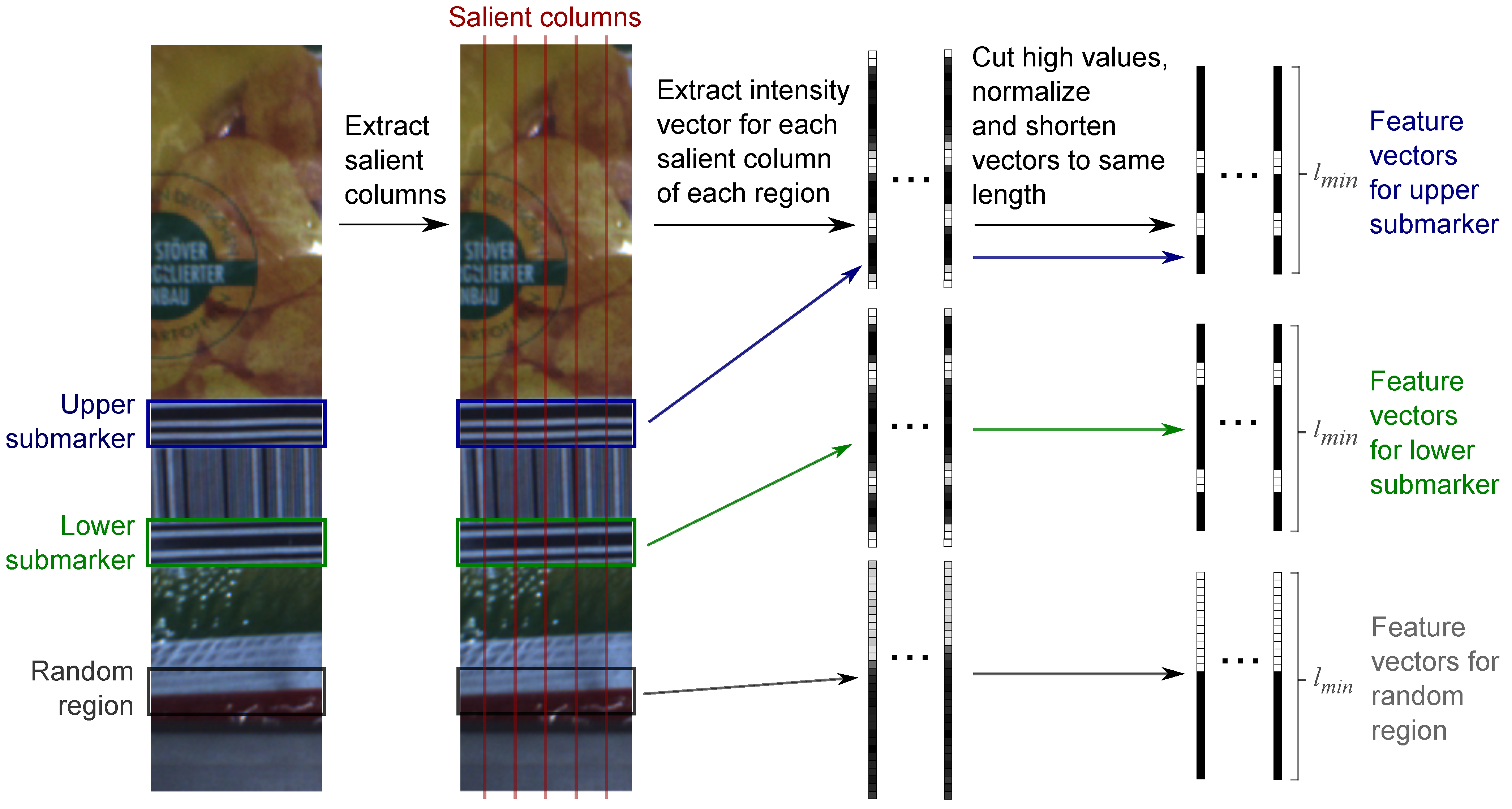
4.3.3. Template Matching Based Marker Detection

The template matching based marker detection (UD-Marker_Template) is quite similar to the aforementioned SVM approach in terms of moving the upper and lower submarkers as a pattern over a salient column and measuring the correlations between the two patterns and the profile of the column. The output comprises two correlation vectors ${\mathbf{k}}^{(j)},{\mathbf{h}}^{(j)}$ for each column j. Before the detection method is described in detail, the overall workflow for the template matching based marker detection approach is presented in the following. The template matching based marker detection starts with converting the input RGB image into a gray-scale image as depicted in Figure 17a. Afterwards, the gray-scale image is filtered by applying a sharpness filter by means of a Laplacian kernel and then utilizing a median filter. The result is a filtered gray-scale image as shown in Figure 17b. In order to equalize different illumination conditions, the contrast of filtered gray-scale image is enhanced by a histogram equalization (illustrated in Figure 17c). By using Otsu’s adaptive thresholding method [20], a binary version of the image is created. An exemplary result image for applying the template matching is depicted in Figure 17d.

The pattern for the upper marker is represented by the vector $\mathbf{u}\in {\mathbb{R}}^N$:

$$\mathbf{u}={(u_0,\dots ,u_i,\dots ,u_{c_1-1})}^T,c_1\le N$$

(9)

and the pattern for the lower marker is represented by the vector $\mathbf{w}\in {\mathbb{R}}^N$:

$$\mathbf{w}={(w_0,\dots ,w_i,\dots ,w_{c_2-1})}^T,c_2\le N$$

(10)

with binary intensity values $u_i,w_i\in \{0,1\}$. The correlations vectors ${\mathbf{k}}^{(j)},{\mathbf{h}}^{(j)}$ are defined as follows:

$${\mathbf{k}}^{(j)}={\left(k_0^{(j)},\dots ,k_i^{(j)},\dots ,k_{N-1}^{(j)}\right)}^T,{\mathbf{h}}^{(j)}={\left(h_0^{(j)},\dots ,h_i^{(j)},\dots ,h_{N-1}^{(j)}\right)}^T.$$

(11)

The correlation values for the patterns are then calculated for each row by

$$k_i^{(j)}=\frac{{\sum }_{i^{\prime }=0}^{N-1}\left(u_{i^{\prime }}·x_{i+i^{\prime }}^{(j)}-\frac{1}{c_1}·{\sum }_{i^{″}=0}^{N-1}{x}_{i+i^{\prime }}^{(j)}\right)}{\sqrt{{\sum }_{i^{\prime }=0}^{N-1}{u}_{i^{\prime }}^2·{\sum }_{i^{\prime }=0}^{N-1}{x}_{i+i^{\prime }}^{(j)}{}^2}}$$

(12)

and

$$h_i^{(j)}=\frac{{\sum }_{i^{\prime }=0}^{N-1}\left(w_{i^{\prime }}·x_{i+i^{\prime }}^{(j)}-\frac{1}{c_2}·{\sum }_{i^{″}=0}^{N-1}{x}_{i+i^{\prime }}^{(j)}\right)}{\sqrt{{\sum }_{i^{\prime }=0}^{N-1}{w}_{i^{\prime }}^2·{\sum }_{i^{\prime }=0}^{N-1}{x}_{i+i^{\prime }}^{(j)}{}^2}}.$$

(13)

Identifying the position of the marker is analogously done to the SVM approach (see Equations (6)–(8)) whereas the classification vectors are exchanged by the correlation vectors presented in this section.

Figure 17. Image states in template matching based marker detection: (a) grayscale image, (b) filtered grayscale image, (c) histogram equalized grayscale image and (d) binary image.

Figure 17. Image states in template matching based marker detection: (a) grayscale image, (b) filtered grayscale image, (c) histogram equalized grayscale image and (d) binary image.

5. Evaluation

This section deals with the evaluation of the color based marker detection (using the Color-Marker_Template algorithm) and the detection of the user-defined marker (employing UD-Marker_SVM and UD-Marker_Template, respectively). The evaluation was executed on the real setup of the fully functional picking system as visualized in Figure 4b and described in detail in Section 3.

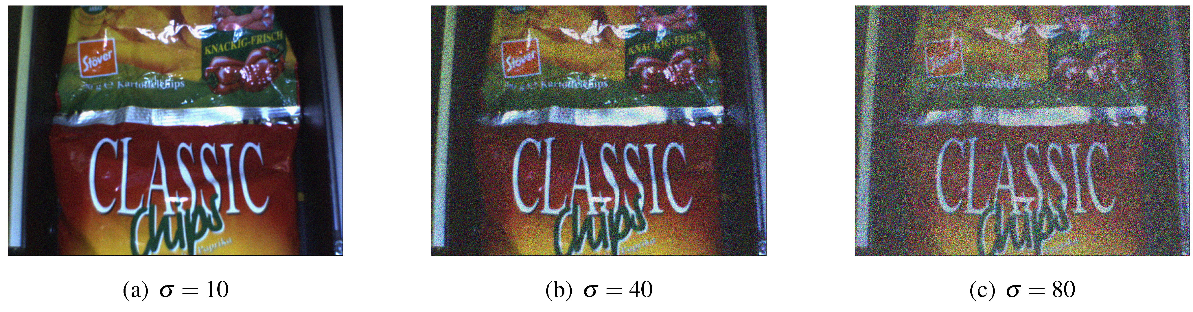
5.1. Vision System Setup

Developed in several research projects [3], the mechanical setup (see Section 3) was extended by a vision system for cutting line detection. The details of the vision system are described next.

According to the requirement of supplying sufficient detection speed, high frame rates of and high data transfer rates to the processing computer are mandatory. Beside this, the deployed camera has to constantly deliver high quality images. Especially in the field of industrial applications, numerous adequate cameras are available in the market (e.g., [21,22]). In the test setup, an acA640-100gc CCD camera produced by Basler AG was used providing frame rates up to 100 frames per second. It is interfaced by the TCP/IP based GigE vision standard [23] and offers different output formats like YUV422, grey scale, RGB24 or RGBA32. Furthermore, shutter speed and a ROI are manually adjustable. To be independent from ambient light, it is equipped with a LED ring lamp. The camera is mounted in a distance of 25 cm to the guiding plate (cf. Figure 4a) of the cover belt conveyor. In combination with a Schneider-Kreuznach wide-angle lens, a captured detection field of 21 cm (width) times 17 cm (height) results. The hardware platform for image processing is an OpenCL compatible x86 personal computer with a quad core processor. The system specifications are detailed along with the experimental runtime analysis in Section 5.2.3.

5.2. Detection Quality, Cutting Line Accuracy and Runtime

In the following, the marker detection methods (Color-Marker_Template, UD-Marker_SVM and UD-Marker_Template) will be experimentally evaluated. Firstly, the quality of the detection algorithms will be assessed (Section 5.2.1). Secondly, the accuracy of the cutting process will be analyzed (Section 5.2.2). Finally, the runtime performance of the detection methods will be presented (Section 5.2.3).

Colored pouches with a silver sealed seam as a color based marker (cf. Figure 6a) will be used as test objects for the Color-Marker_Template algorithm. For the UD-Marker_SVM and UD-Marker_Template detection methods, transparent pouches with the user-defined marker will be utilized as test candidates.

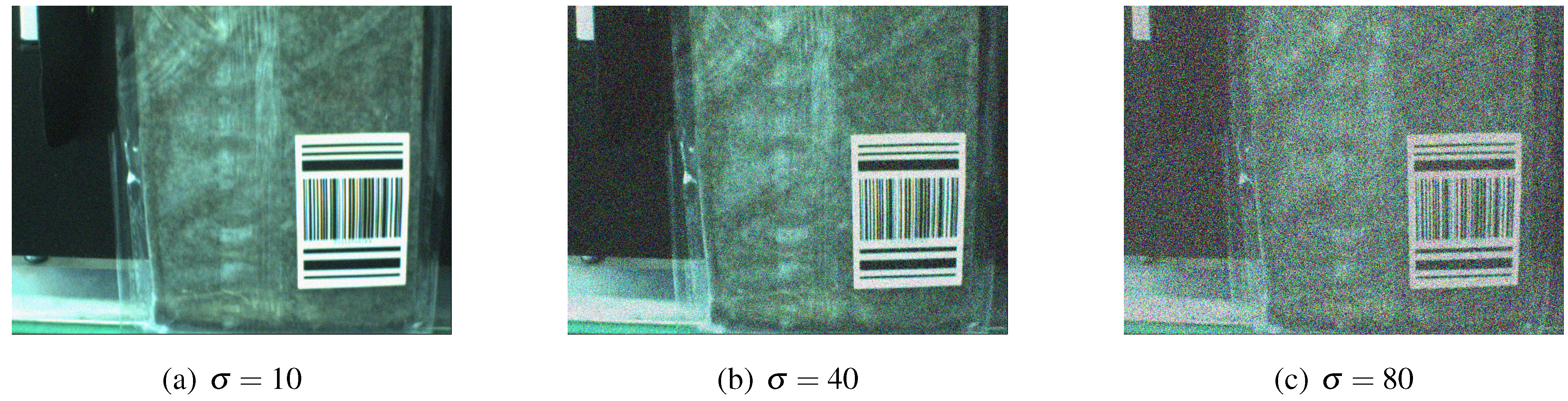
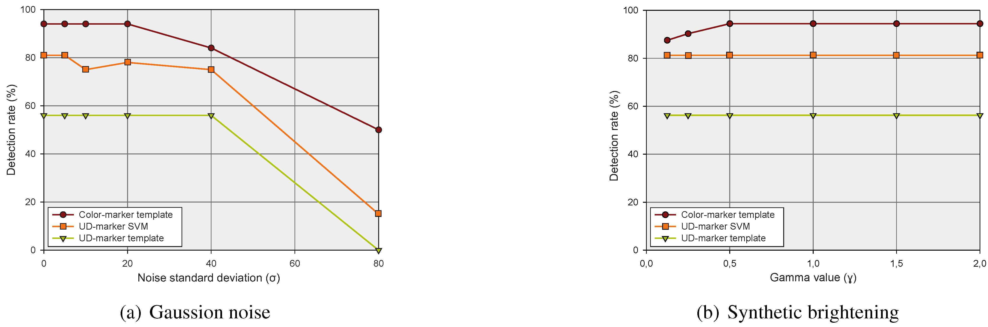
5.2.1. Detection Quality

In this section, the marker detection algorithms are evaluated in terms of robustness if the image is synthetically modified by adding Gaussian noise and global brightening.

Generally, the overall performance of the system is depending on several parameters; the detection process is one of them. On the one hand, performance could be seen from a bottleneck perspective. The system consists of the pouch transport unit, the cutting unit and the detection unit. Depending on the length of the bags, the transport unit or the cutting unit limits the possible performance. Nevertheless, the cutting unit is able to perform 4 cuts per second. As long as the long side of a pouch is shorter than 200 mm (a typical size), the cutting unit becomes the bottleneck. Hence, available process time for marker detection and cutting is about 250 ms. On the other hand, manual and automatic order picking has to be compared: For manual picking, the process time could be calculated [24] and lasts certainly longer than one second. Thus, any performance achievement above 1 pouch per second is not only acceptable but also the basis for economical feasibility. Regarding the detection quality, a detection rate close to 100% is mandatory for industrial applications to assure robust picking processes.

Gaussian Noise: In practice, the quality of the captured images is not constant, e.g., caused by random noise of the sensor. Hence, the original images were modified by adding Gaussian noise with an average standard deviation of $\sigma =5,10,20,40$ and 80 as illustrated in Figure 18 and Figure 19. Figure 20a shows the detection rate of the color based marker depending on the specified average standard deviation of Gaussian noise by using a dark line with rectangle markers. The detection rate for a standard deviation up to $\sigma =20$ amounts stable at 94%. For $\sigma =40$, the detection rate decreases to 85% and for $\sigma =80$, the color based marker is detected only in 50% of the total cases. For the user-defined marker detection methods, the trends for the different noise levels are similar. For up to $\sigma =40$, the detection rate remains on a high level and decreases for greater values of σ. It can be concluded from Figure 20a that the SVM based detection approach has a higher detection rate than the template matching based approach. This can be explained by the major flexibility of the SVM based approach.

Figure 18. Color marker with Gaussian noise.

Figure 18. Color marker with Gaussian noise.

Figure 19. User-defined marker with Gaussian noise.

Figure 19. User-defined marker with Gaussian noise.

Synthetic Brightening: The illumination conditions are not constant in practice. Hence, the robustness of the detection algorithm is evidenced by robust detections in varying illumination conditions. The original image was modified by adjusting the γ (gamma) value of the images as illustrated in Figure 21 and Figure 22. The evaluation results are shown in Figure 20b. A γ value of one ($\gamma =1$) equals the original image lightening and values below one ($\gamma <1$) result in brighter images with lesser contrast. A value above one ($\gamma >1$) will also lead to an image with a lower contrast but it will be much darker than the original one. As it can be seen in Figure 20b, the detection rate for the SVM based approach and the template matching based approaches is the same as for the original images for all configurations. Therefore, the detection rate of the SVM based approach is around 81% and the template matching attains about 54%. In terms of an industrial application, the environment and hardware have to be adapted to achieve a detection rate close to 100% which is a common requirement in industry. The situation for the color marker is different since the method is based on the brightness differences in the figure itself and therefore, the detection rate will decrease when brighter images are considered.

Figure 20. Evaluation of the robustness of the detection algorithm under varying (a) random Gaussian noise with standard deviation $\sigma =5;10;20;40;80$ and (b) illumination conditions with $\gamma =0.125;0.25;0.5;1.5;2$.

Figure 20. Evaluation of the robustness of the detection algorithm under varying (a) random Gaussian noise with standard deviation $\sigma =5;10;20;40;80$ and (b) illumination conditions with $\gamma =0.125;0.25;0.5;1.5;2$.

Figure 21. Color marker with synthetic brightening.

Figure 21. Color marker with synthetic brightening.

Figure 22. User-defined marker with synthetic brightening.

Figure 22. User-defined marker with synthetic brightening.

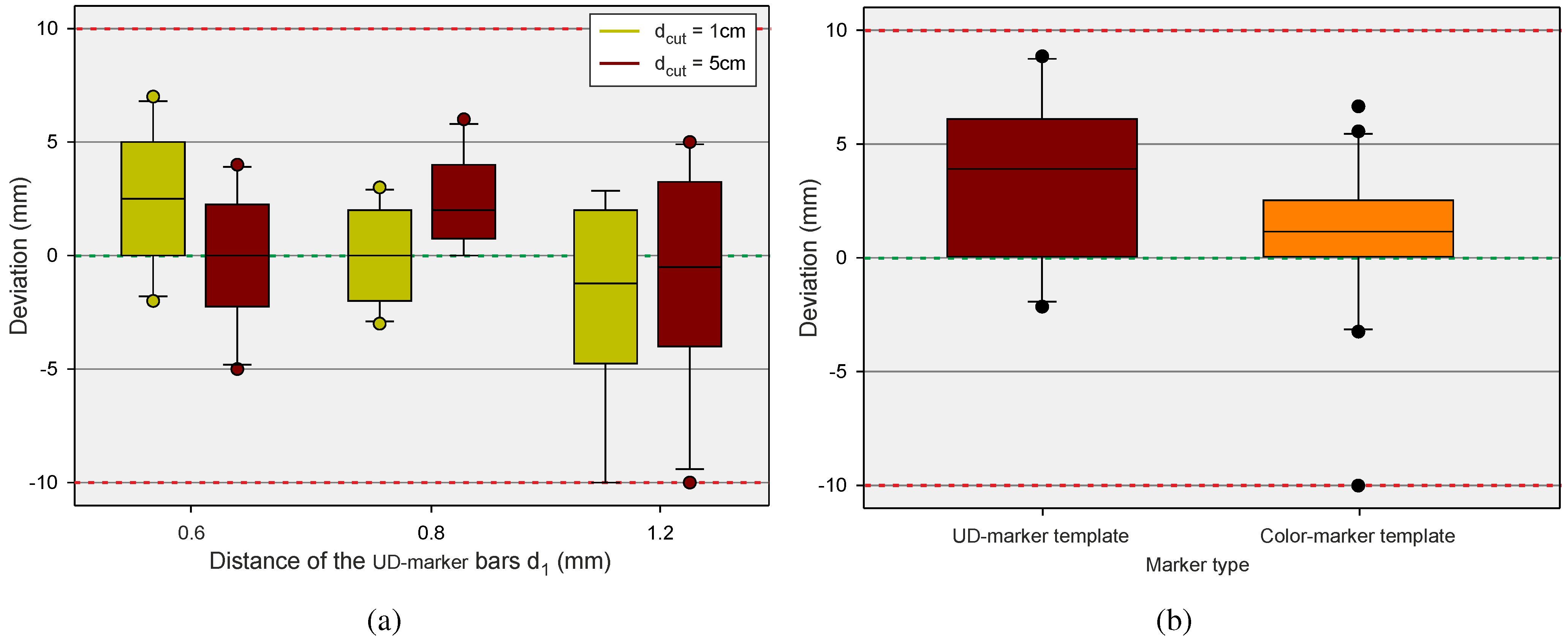
5.2.2. Cutting Line Accuracy

The evaluation of the cutting accuracy was done by measuring the deviation of the performed to the optimal cutting line with chains of 10 pouches. In contrast to the evaluation of the detection quality in the previous Section 5.2.1, the test runs were executed on the real machine setup.

Within the test runs, the distance of the user-defined marker bars $d_1\in \left\{0.6\text{mm},0.8\text{mm},1.2\text{mm}\right\}$ and the distance of the marker to the optimal cutting line $d_{cut}\in \left\{1\text{cm},5\text{cm}\right\}$ were varied (cf. Figure 13a). The results are illustrated in Figure 23a as box-and-whisker plots. Within the test series, all markers were detected. Overall result is a notable small deviation (less than 10 mm for the maximum deviation in total) of the detected cutting line compared to the optimal cutting line. The most significant reason for the deviations is the occurrence of irregularly sealed seams of the pouches and a small deviation of the marker positions caused by manual attaching.

Figure 23. Accuracy of the detection process with UD-Marker_SVM on (a) transparent pouches. Varied parameters are the distance of the user-defined marker bars $d_1\in \left\{0.6\text{mm},0.8\text{mm},1.2\text{mm}\right\}$ and the distance of the marker to the optimal cutting line $d_{cut}\in \left\{1\text{cm},5\text{cm}\right\}$. Visualization of the accuracy of the detection process of the template approaches (b): UD-Marker_Template on transparent pouches with user-defined marker and Color-Marker_Template on colored pouches. The y-axis in each box-whisker-plot indicates the deviation of the detected to the optimal cutting line.

Figure 23. Accuracy of the detection process with UD-Marker_SVM on (a) transparent pouches. Varied parameters are the distance of the user-defined marker bars $d_1\in \left\{0.6\text{mm},0.8\text{mm},1.2\text{mm}\right\}$ and the distance of the marker to the optimal cutting line $d_{cut}\in \left\{1\text{cm},5\text{cm}\right\}$. Visualization of the accuracy of the detection process of the template approaches (b): UD-Marker_Template on transparent pouches with user-defined marker and Color-Marker_Template on colored pouches. The y-axis in each box-whisker-plot indicates the deviation of the detected to the optimal cutting line.

The evaluation of the cutting accuracy for the Color-Marker_Template was determined on a chain with 30 colored pouches by measuring the deviation of the detected to the optimal cutting line. The right box-and-whisker plot in Figure 23a illustrates the results. Within the test series, two markers were not detected and led to false negatives (i.e., no cut was performed). The critical false positives, cases in which a cut was performed although no marker was present, did not occur. Disregarding the false negatives, a notable fact is the small deviation of the detected to the optimal cutting line when the marker is correctly detected. The most significant reason for false negatives and the deviations is due to the irregularly buckling of the pouches which is currently not taken into account by the detection algorithm.

The left box-and-whisker plot in Figure 23b further illustrates the evaluation results for the cutting accuracy with the template matching based detection (UD-Marker_Template) based on transparent pouches with the user-defined marker. Within the test runs, each marker was detected while the deviation of the associated cutting line to the optimal cutting line was less than 8 mm in all cases and less than 5 mm on average.

Derived from the results of the cutting line detection accuracy for the different strategies, a sealed seam width of 20 mm (10 mm for the upper plus 10 mm for the lower seam) is suitable for robust operation.

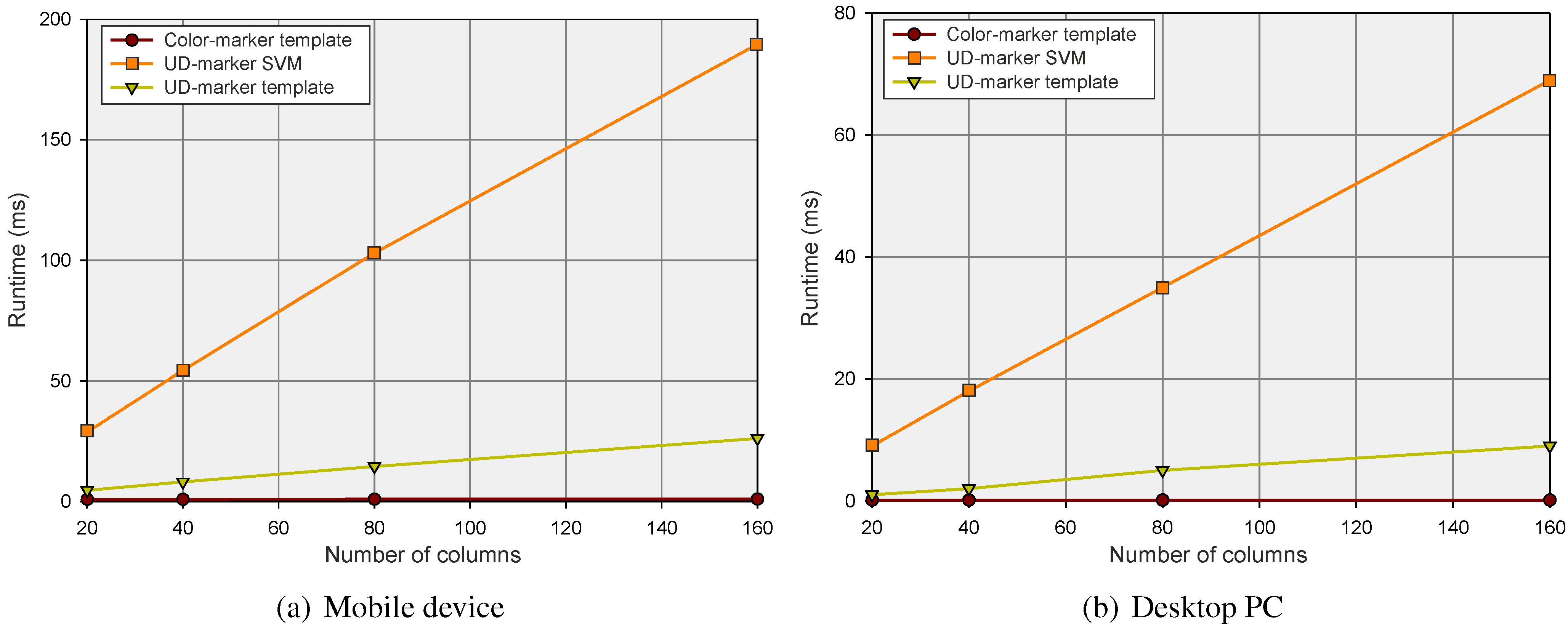
5.2.3. Runtime Performance

The runtime performance of the three marker detection mechanisms were measured on two hardware platforms which could be utilized for efficient data processing: (1) a mobile device (Intel i5M 2.53 GHz, 4 GB RAM, Windows 7 64 bit) and (2) a desktop PC (Intel i5 2.80 GHz, 8 GB RAM, Windows 7 64 bit). The results for the mobile device are shown in Figure 24a and the results for the desktop PC are depicted in Figure 24b. From both figures, it can be derived that the runtime scales linear with the number of salient columns. Another point which can be concluded from Figure 24 is that the histogram-based marker detection is much faster than the detection algorithms for the user-defined markers. This is due to the simpler detection strategy. The runtimes of the histogram-based detection methods are below 1 ms for all tested configurations. The runtime of the template matching and the SVM based approach for the user defined marker grows linear with the number of salient columns. Due to the more flexible nature of the SVM based approach and its robustness against noise and illumination situations, the requirements with regard to the hardware platform are higher in comparison to the other methods.

Figure 24. Runtimes for different marker detection methods on (a) a mobile device (Intel i5M 2.53 GHz, 4 GB RAM, Windows 7 64 bit) and (b) an desktop PC (Intel i5 2.80 GHz, 8 GB RAM, Windows 7 64 bit).

Figure 24. Runtimes for different marker detection methods on (a) a mobile device (Intel i5M 2.53 GHz, 4 GB RAM, Windows 7 64 bit) and (b) an desktop PC (Intel i5 2.80 GHz, 8 GB RAM, Windows 7 64 bit).

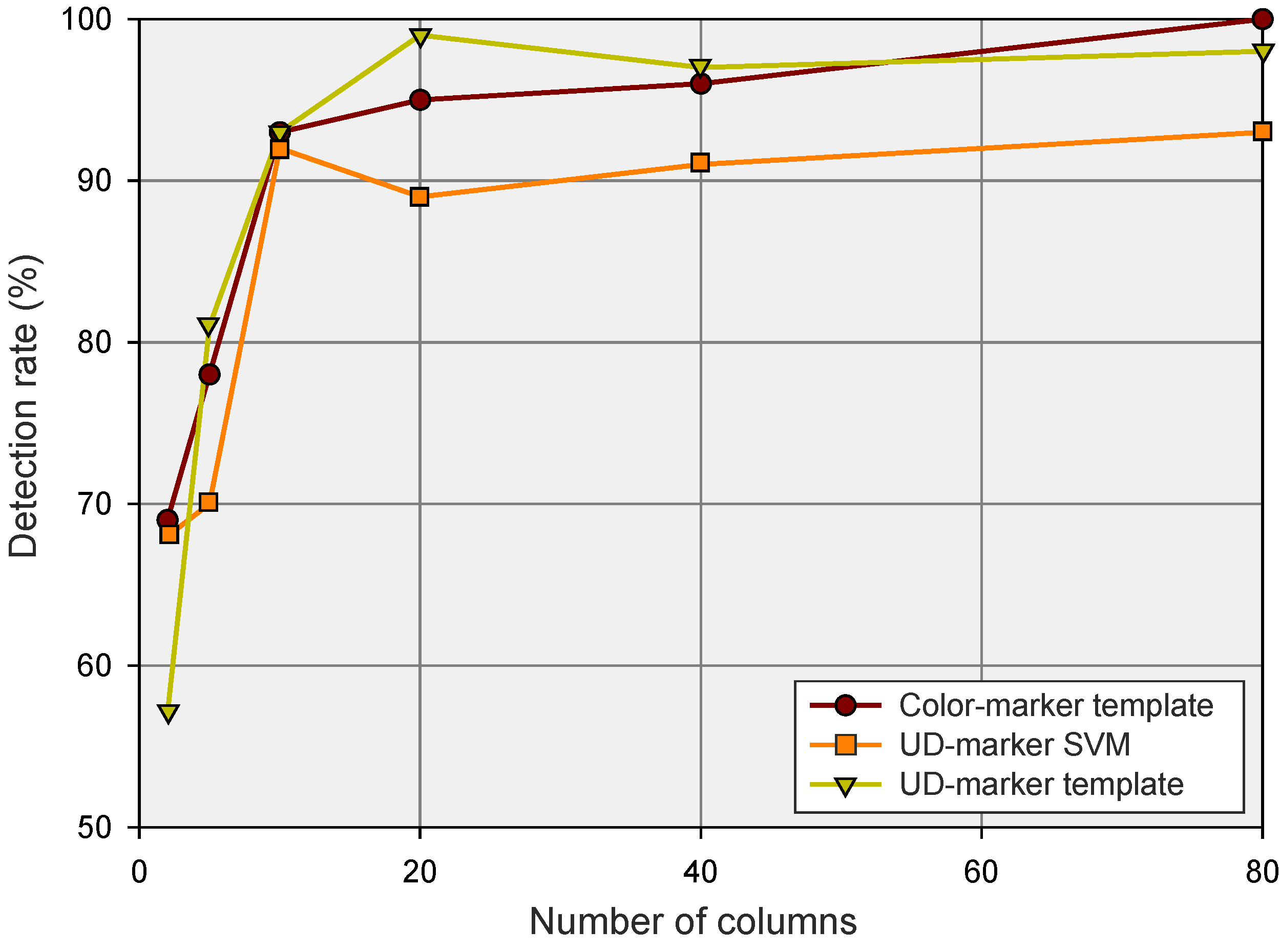
5.3. Trade-off Considerations: Detection Quality vs. Number of Columns

The robustness of the detection quality depends on the number of salient columns which are analyzed by the presented marker detection methods Color-Marker_Template, UD-Marker_SVM and UD-Marker_Template (cf. Figure 25). As the vertical size of the user defined marker maximum counts approximately 100 pixels in the images taken by the camera, a ROI consisting of maximum 80 salient columns (cf. Paragraph 4.3.2) was defined. The number of columns directly influences the runtime performance. Hence, a trade-off between the number of columns resulting in definite detection rate and the runtime of the detection algorithm is mandatory. In case of Color-Marker_Template processing, the marker detection on 80 salient columns yields a detection rate of 100% while the runtime stays beneath 1 ms. For the user-defined marker detection with UD-Marker_SVM, a detection rate of approximately 90% is reached for already 10 salient columns with a runtime of about 20 ms. UD-Marker_Template leads to the best detection results for a ROI consisting of 20 salient columns with a runtime less than 5 ms. In case of UD-Marker_SVM and UD-Marker_Template, increasing the number of columns above the mentioned thresholds does not yield improved detection results.

Figure 25. Trade-off consideration between the detection quality and the number of columns: the detection rate (%) depends on the number of salient columns as input for the marker detection algorithms Color-Marker_Template, UD-Marker_SVM and UD-Marker_Template.

Figure 25. Trade-off consideration between the detection quality and the number of columns: the detection rate (%) depends on the number of salient columns as input for the marker detection algorithms Color-Marker_Template, UD-Marker_SVM and UD-Marker_Template.

6. Conclusion

In this paper, a novel approach for detecting sealed seams allowing automated order picking of pouch packed goods was presented. Beyond a few existing expensive and specialized solutions in the field of automated order picking of pouch packed goods, an efficient and inexpensive vision based concept was developed which supports the detection of different types of pouches. The core of the new approach was a vision based marker detection system with the realization of two different marker detection strategies, template matching as a heuristic concept, and SVMs as a supervised classification based concept.

The evaluation results of the presented vision based marker detection system show that efficient and reliable marker detection can be guaranteed for color based and user-defined markers on different types of pouches. The number of salient columns analyzed by the marker detection algorithms lead to a balance between the detection robustness and calculation time. Already 10 salient columns are sufficient for a detection rate greater than 90% with a calculation time less than 5 ms. Analyzing 80 salient rows with Color-Marker_Template leads to a detection rate of 100% with a calculation time of less than 1 ms and a detection rate of almost 100% using the new user-defined marker approaches (UD-Marker_SVM and UD-Marker_Template) with a calculation time of less than 40 ms. Up to a conveying speed of 200 mm per second, a robust detection using the two different strategies can be proven. In addition to that, experimental verification proved the robustness of the three presented detection algorithms (Color-Marker_Template, UD-Marker_SVM and UD-Marker_Template) in terms of image sensor noise and varying illumination scenarios. The effect of combining the (simulated) Gaussian noise and synthetic brightening may be investigated in further reseach. However, the results of Section 5 should be considered as guidelines to (re-) design the picking system. For example, the illumination conditions may be controlled by replacing the acrylic glass panels with non-transparent panels (cf. Figure 4b). To compensate deviation in cutting accuracy, a sealed seam width of 20 mm is suitable which seems feasible from a pouch production perspective. However, the pouches used in this paper exhibit rather large sealed seams which allows us to neglect the deformations. This aspect should be addressed in further research, too. With a total hardware cost of approximately 800 Euro (300 Euro for the camera and 500 Euro for a desktop PC), the presented embedded approach provides a competitive alternative to expensive high integrated sensors just like smart cameras.

Future fields of research are the motion prediction as a further enhancement of the performance of the detection method and trade-off analyses. At this, the comparison to other automated order picking systems, particularly relating to the throughput, is a central aspect of further research. The overall quality of the system is sufficient for most desired application areas but due to the cost/performance trade-off, it may be desirable to even use cheaper hardware such as slower cameras. By using these platforms, it is mandatory to integrate additional advanced motion prediction / tracking algorithms, such as Hidden Markov Models [25] or Condensation algorithms [26].

References

1. Bvh–Bundeverband des Deutschen Versandhandels. Aktuelle Zahlen zum interaktiven Handel: “Jahresprognose 2014 für den interaktiven Handel mit Waren”. Available online: http://www.bvh.info/zahlen-und-fakten/allgemeines/ (accessed on 30 June 2014).
2. European Union. Key Figures on European Business—With Special Feature on SMEs; Eurostat Pocketbooks; Eurostat: Luxembourg, 2011. [Google Scholar]
3. Leiking, L. Method of Automated Order-Picking of Pouch-Packed Goods. PhD Thesis, Technical University of Dortmund, Dortmund, Germany, 2007. [Google Scholar]
4. Statistisches Bundesamt—DESTATIS. Produktion des verarbeitenden Gewerbes sowie des Bergbaus und der Gewinnung von Steinen und Erden—Verarbeitendes Gewerbe, 2014. Fachreihe 4, Reihe 3.1, 4th quarter of 2013; Statistisches Bundesamt: Wiesbaden, Germany, 2014. [Google Scholar]
5. Verein deutscher Ingenieure (VDI). Kommissioniersysteme: Grundlagen. Richtlinie, VDI 3590. Beuth Verlag: Düsseldorf, Germany, 1994. [Google Scholar]
6. ten Hompel, M.; Schmidt, T. Warehouse Management; Springer-Verlag: Berlin/Heidelberg, Germany, 2008. [Google Scholar]
7. SSI-Schäfer Peem GmbH. Schachtkommissionierer/A-Frame, 2011. Available online: http://www.ssi-schaefer.de/foerder-und-kommissioniersysteme/automatische-kommissionierung/a-frame.html (accessed on 18 July 2014).
8. Viastore Systems. Vollautomatisches Kommissioniersystem viapick, 2011. Available online: http://www.viastore.de/kommissioniersysteme/viapick.html (accessed on 18 July 2014).
9. Apostore GmbH. Carry Fix Pusher, 2014. Available online: http://www.apostore.de/de/produkte/spezialloesungen/carryfix-pusher.html (accessed on 18 July 2014).
10. Siemens Technical Press, Industry Sector. Vereinzelung auf kleinstem Raum mit dem Visicon Singulator von Siemens, 2009. Available online: http://w1.siemens.com/press/de/pressemitteilungen/2009/mobility/imo200901008.htm (accessed on 18 July 2014).
11. Karaca, H.; Akinlar, C. A multi-camera vision system for real-time tracking of parcels moving on a conveyor belt. In Computer and Information Sciences—ISCIS 2005; Springer-Verlag: Berlin/Heidelberg, Germany, 2005; Volume 3733, pp. 708–717. [Google Scholar]
12. Rontech. SpaceFeeder—Universal Infeed System, 2011. Available online: http://www.rontech.ch/index.cfm?navid=41&detailid=7 (accessed on 18 July 2014).
13. Somtec. Automatische Beutelvereinzelung und Kartonbefüllung, 2008. Available online: www.somtec.de (accessed on 18 July 2014).
14. Rovema Verpackungsservice GmbH. Packaging Concepts, 2011. Available online: http://www.ptg-verpackungsservice.de/deutsch/dienstleistung/beutel/index.html (accessed on 18 July 2014).
15. Rockwell Automation, Inc. The VFFS (Vertical From Fill Seal) Machine Application, 2008. Available online: http://literature.rockwellautomation.com/idc/groups/literature/documents/wp/oem-wp004_-en-p.pdf (accessed on 18 July 2014).
16. Schultze, S.; Schnabel, H. Sensor for Marks on or in Material and Method of Sensing a Mark on or in a Material. Patent No. DE102008024104A1, 2010. [Google Scholar]
17. Schölkopf, B.; Sung, K.; Burges, C.; Girosi, F.; Niyogi, P.; Poggio, T.; Vapnik, V. Comparing Support Vector Machines with Gaussian Kernels to Radial Basis Function Classifiers. IEEE Trans. Signal Process. 1997, 45, 2758–2765. [Google Scholar] [CrossRef]
18. Cristianini, N.; Shawe-Taylor, J. Support Vector Machines; Cambridge University Press: Cambridge, UK, 2000. [Google Scholar]
19. Gaspar, P.; Carbonell, J.; Oliveira, J. On the parameter optimization of Support Vector Machines for binary classification. J. Integr. Bioinf. 2012, 9, 1–11. [Google Scholar]
20. Otsu, N. A Threshold Selection Method from Gray-Level Histograms. IEEE Trans. Syst. Man Cybern. 1979, 9, 62–66. [Google Scholar]
21. Basler AG. Available online: http://www.baslerweb.com (accessed on 18 July 2014).
22. Allied Vision Technologies. Digital Machine Vision Cameras. Available online: http://www.alliedvisiontec.com/emea/home.html (accessed on 18 July 2014).
23. GigE Vision—True Plug and Play Connectivity. http://www.visiononline.org/vision-standards-details.cfm (accessed on 18 July 2014).
24. Gudehus, T. Logistik—Grundlagen, Strategien, Anwendungen; Springer-Verlag: Berlin/Heidelberg, Germany, 2010. [Google Scholar]
25. Rabiner, L.; Juang, B. An Introduction to Hidden Markov Models. IEEE ASSP Mag. 1986, 3, 4–16. [Google Scholar] [CrossRef]
26. Koller-Meier, E.; Ade, F. Tracking multiple objects using the condensation algorithm. Robot. Auton. Syst. 2001, 34, 93–105. [Google Scholar] [CrossRef]