1. Introduction
Water is critical to humans in many ways: it provides food, natural resources, and helps regulate the climate. As such, developing tools to help monitor the health of bodies of water is a key scientific challenge. Though a number of monitoring tools have been developed, including underwater modeling, mapping, and resource monitoring, the majority of this work is currently done manually or using expensive, hard-to-maneuver underwater vehicles. A new level of automation is needed in the form of versatile and easily deployable underwater robots and sensor networks that (1) can effectively collect the right data; (2) efficiently store the data and (3) provide quasi-real-time access to it.
In this article (This article is an extended version of our prior work presented at SenSys 2010 [
1]. This article extends our control algorithm to include robot operation and includes additional simulation and field experiment results.), we describe platforms and algorithms that enable automation of water observation tasks. Specifically, we develop, analyze, and test a decentralized, adaptive algorithm for positioning an underwater sensor network. Our sensor network nodes dynamically adjust their depths through a new decentralized, gradient-descent-based algorithm with guaranteed properties. The dynamic depth adjustment algorithm runs online, which enables the nodes to adapt to changing conditions (e.g., tidal front) and does not require a-priori decisions about node placement in the water. Through neighbor communication the algorithm collaboratively optimizes the nodes’ depths for sensing in support of computing maximally detailed volumetric models. We prove that the controller algorithm converges to a local minimum. In addition, we show that we can extend the algorithm to optimize the path of a mobile robot traveling through the sensor field. Through simulations and experiments on our A
quaN
ode hardware platform, we show that the local minimum is near the global minimum of the system; often the local minimum equals the global.
We apply the algorithm to the problem of monitoring chromophoric dissolved organic matter (CDOM) in the Neponset River that feeds into Boston Harbor (see
Figure 1). CDOM is part of the dissolved organic matter in rivers, lakes, and oceans. An understanding of CDOM dynamics in coastal waters and its resulting distribution is important for remote sensing and for estimating light penetration in the ocean. In this paper, we simulate positioning sensors along the Neponset River and adjusting their depths to optimize the sensing of CDOM as it is discharged into Boston Harbor. We also use the CDOM model as input for a four-node test deployment in both the Charles River and the Neponset River.
The decentralized controller positions the nodes so they are in good locations to collect data to model the values of the system over the whole region, not just the particular points where there are sensors. The sensor nodes use a covariance function that describes the relationship between the possible positions of the sensor nodes and the whole region of interest. As a first pass, we model the covariance as a multivariate Gaussian, as is often used in objective analysis in underwater environments [
2]. We also compute a numeric covariance for the Neponset River based on data from a numerical model of the river. The model is based on the readings from a few specific sensor locations and is extended to all points in the river using a physics-based hydrodynamic model [
3].
The algorithm assumes a fixed covariance model; however, we show in a river test that the algorithm can be iterated with different covariance models to capture dynamic phenomena. In the Neponset River, the concentration of CDOM is highly dependent on the tide level, which causes river level variations of about 2 m. The physics-based model lets us numerically compute the covariance of the CDOM readings in the Neponset River based on different tide levels. The nodes adjust their covariance model, and therefore their depths, based on the tide charts. The model data is accurate on average; however, it may not accurately capture small-scale temporal and spatial variations. The sensor nodes and algorithm fill this gap and provide detailed measurements at informative locations. In addition, when an underwater robot is available, the underwater sensor network informs the robot of the best path to travel for sensing while also adapting the positions of the sensors to account for the path of the robot. Over time, the physics-based CDOM model can be enhanced by using the new measurements.
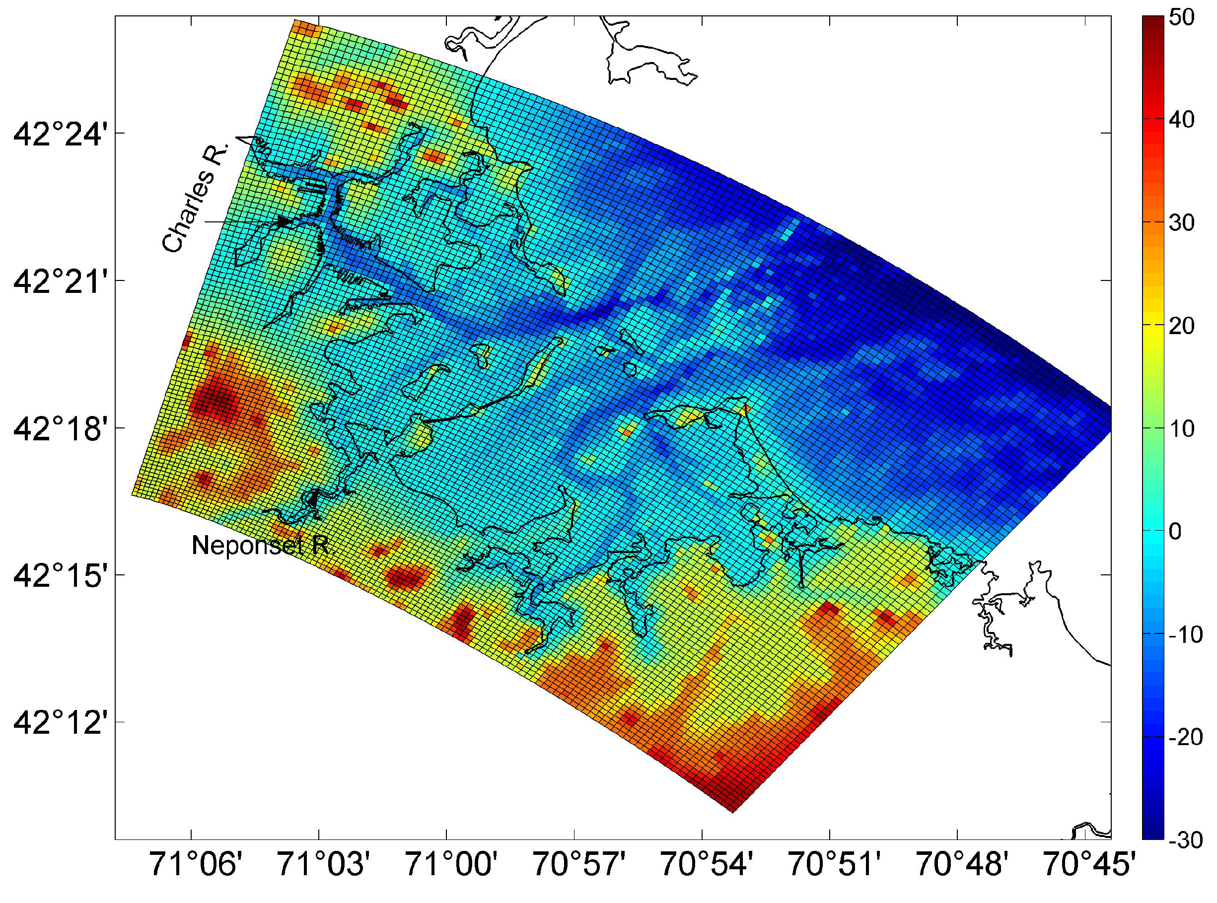
Figure 1.
Boston Harbor bathymetry and grid for hydrodynamic model.
Figure 1.
Boston Harbor bathymetry and grid for hydrodynamic model.
The controller uses the covariance in a decentralized gradient descent algorithm. We implement this solution in simulation and on our AquaNode underwater sensor network that has depth adjustment capabilities and test it in lab, pool, and river. The algorithm requires very little communication, allowing each node to only send its own depth information, as well as providing fault tolerance in instances where packets are lost. Both are important in underwater sensor networks that can only communicate acoustically, i.e., low bandwidth (300 b/s) and limited reliability (<50% packet success). Our algorithm has low memory and computation requirements, which allows it to run in real-time on our power efficient sensor network.
This article makes a number of contributions to the field of underwater sensor networks and robotics. Specifically, we (1) present our underwater sensor network and robot system, (2) develop a decentralized controller that optimizes the depths of our underwater sensors for data collection, (3) prove that the controller converges, (4) extend the algorithm to work with underwater robots, (5) extensively analyze the performance in simulation, in lab and in pool, and (6) perform in-situ experiments in both the Charles River and the Neponset River.
The rest of this article is organized as follows. First, we introduce our underwater sensor network in
Section 2. We then discuss the model of the river and ocean environment and its importance for scientific understanding in
Section 3. We next introduce and analyze our decentralized depth controller algorithm on our underwater sensor network in
Section 4 and with our underwater robot in
Section 5.
Section 6 explores results of simulations to test the performance of the algorithm and explores the sensitivity to different parameters. We then present the results of experiments on our A
quaN
ode platform in lab, pool, and two rivers in
Section 7. This is followed by a discussion of related work in
Section 8. Finally, we discuss future work and conclude in
Section 9.
2. Underwater Sensor Network and Robot Platform
We have developed an inexpensive underwater sensor network system that incorporates the ability to dynamically adjust its depth. The base sensor node hardware is called the A
quaN
ode platform and is described in detail in [
4,
5,
6]. We have extended this basic underwater sensor network with autonomous depth adjustment ability and created a five node sensor network system, whose nodes move up and down in the water column under their own control [
7]. In addition, we have developed an underwater robot, called A
mour, that can interact and acoustically communicate with the underwater sensor network [
8,
9,
10]. Here we will briefly summarize the system and describe some details of the winch-based depth adjustment system and the underwater robot.
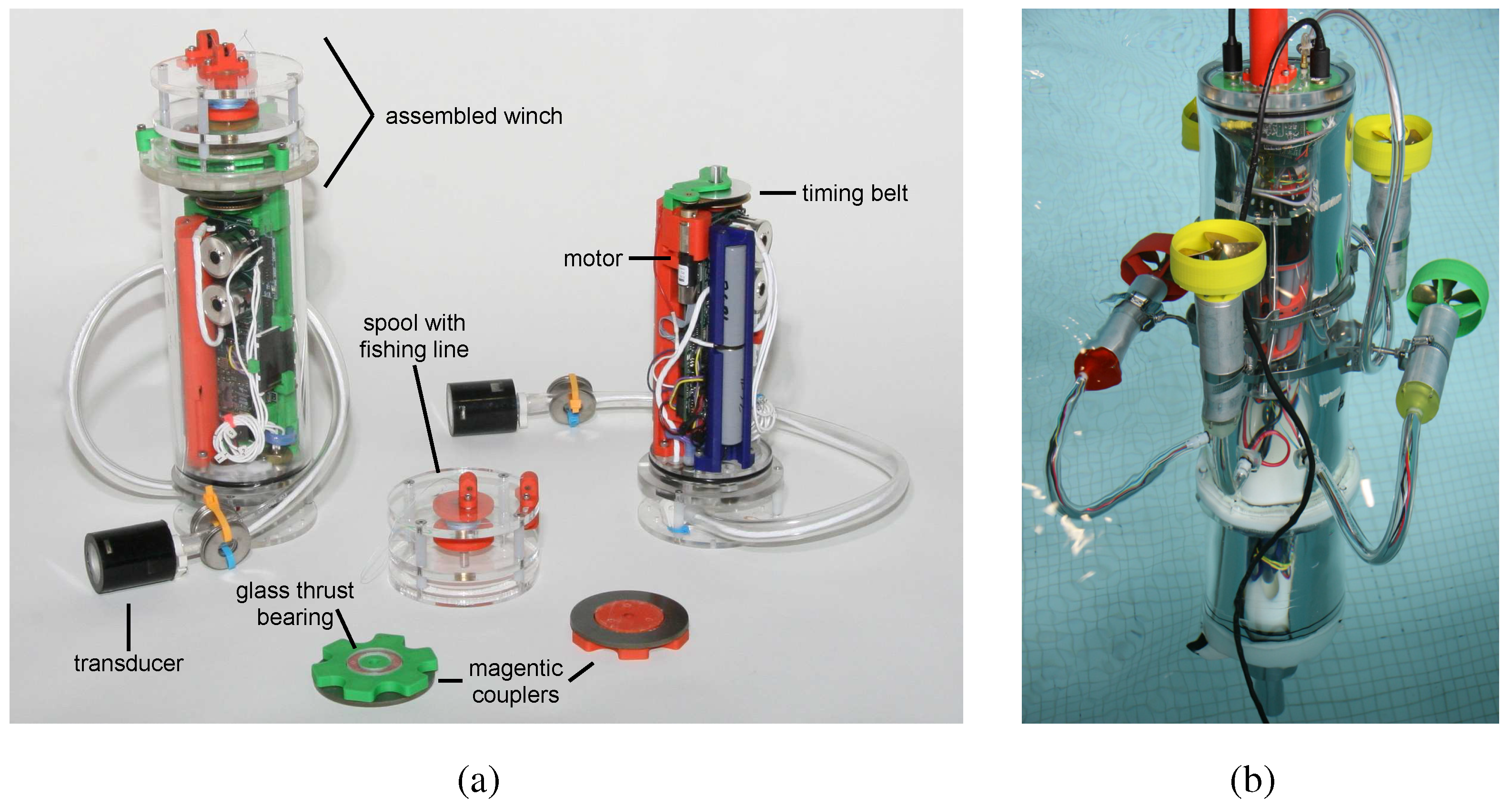
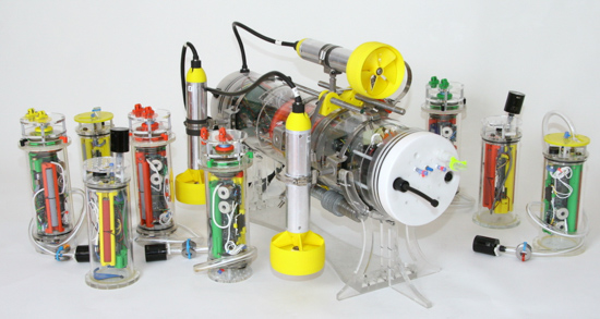
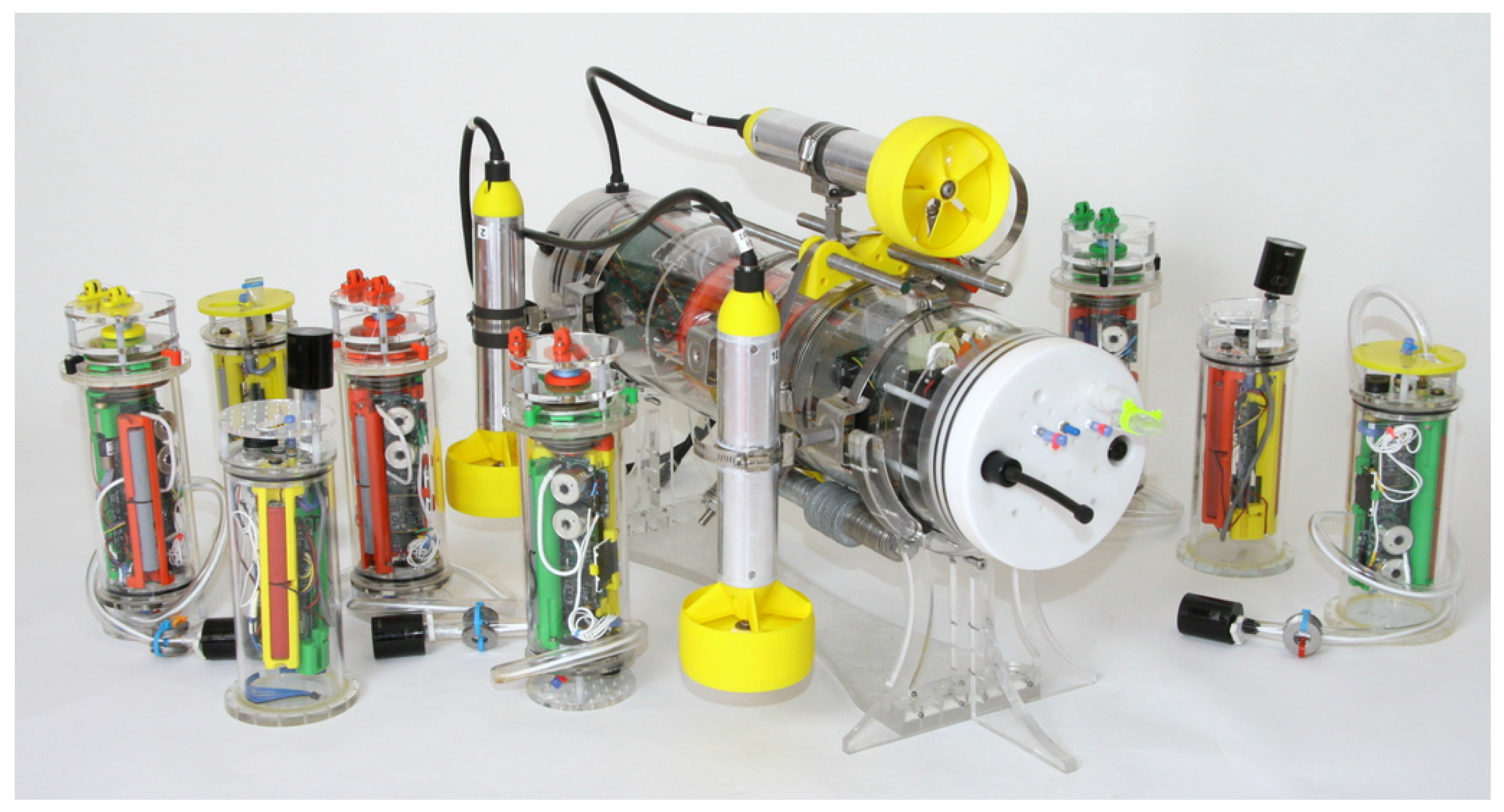
Figure 2 shows a picture of two A
quaN
odes with the depth adjustment hardware and our underwater robot A
mour. Both the underwater sensors and the robot have built-in pressure and temperature sensors and a variety of other analog and digital sensors. Examples of sensors we have connected include CDOM, salinity, dissolved oxygen, and cameras.
Figure 2.
(a) Depth adjustment system with AquaNode and (b) underwater robot Amour.
Figure 2.
(a) Depth adjustment system with AquaNode and (b) underwater robot Amour.
The main communication system we use for communication between sensor nodes and with the underwater robot is a custom developed 10 W acoustic modem [
5]. The modem uses a frequency-shift keying (FSK) modulation with a 30 KHz carrier frequency and has a physical layer baud rate of 300 b/s. The MAC layer is a self-synchronizing TDMA protocol with 4 s slots. In each slot the master can send a packet and receive a response from one other sensor node. Each packet contains 11 bytes of payload. The acoustic modems are also able to measure distances between pairs of nodes. In previous work we have demonstrated how this can be used to perform relative localization between the sensor nodes and provide localization information to underwater robots [
11]. We can use this capability to determine the positions of the nodes in our experiments and guide the underwater robot.
The A
quaN
ode is anchored at the bottom and floats mid-water column. The depth adjustment system allows the length of anchor line to be altered to adjust the depth in the water. The A
quaN
ode is cylindrically shaped with a diameter of 8.9 cm and a length of 25.4 cm without the winch mechanism and 30.5 cm with the winch attached. It weighs 1.8 kg and is 200 g buoyant with the depth adjustment system attached. The depth adjustment system allows the A
quaN
odes to adjust their depth (up to approximately 50 m) at a speed of up to 0.5 m/s and use approximately 1 W when in motion. With frequent motion and near continuous depth adjustment the nodes have power (60 Wh) for up to two days. In low power modes it can be deployed for about a year, but typical deployments are in the order of weeks. See [
7] for additional details on the A
quaN
ode hardware.
3. Modeling Underwater Phenomena
One prominent phenomenon in coastal oceans is the existence of tidal fronts, which are located at the meeting place of freshwater and oceanic water, normally determined by the strongest salinity gradient. Such fronts are typically associated with high concentrations of suspended sediments and hence with high turbidity, so-called the maximum turbidity zone (MTZ) [
12]. The frontal zones also tend to be biologically active areas attracting zooplankton and fish larvae due to turbulent mixing and physical retention [
13,
14]. For a small river, the flow may be approximated as two-dimensional (one vertical and one along the river channel), and hence the front can be approximated as a thin line from the surface tilting down to the bottom with a vertical thickness tens of cm. The frontal position is determined by the river flow and tidal movement, but is moving back and forth along with tidal flow. In Neponset River, the dominant period of frontal movement is 12.4 h, controlled by the M2 tide component.
Underwater sensor networks enable detecting and measuring the tidal front in Neponset River in conjunction with a numerical model. The model we use in this paper was developed for Boston Harbor (BH), based on the Estuarine, Coastal, Ocean Model (ECOM-si) with Mellor and Yamada 2.5 turbulent closure for the vertical mixing [
15,
16,
17]. The model domain covers the entire BH (over 500 km
) and a part of the Massachusetts Bay (MB) with a grid resolution of around 70 m (
Figure 1). The model was forced by surface winds and heat fluxes derived from measurements at NOAA buoy 44013 in western MB, and freshwater discharges at the USGS gauges, as well as boundary forcing (tides, currents, temperature and salinity) derived from the model output of the MB hydrodynamic model [
3]. The model captures the general dynamic processes including tidal cycle, seasonal development of stratification, and wind- and river-driven circulation.
We are particularly interested in CDOM, which is the optically active component of the total dissolved organic matter in the oceans. In estuaries, CDOM is mostly exported from watersheds through freshwater discharges with addition from fringing salt marshes, and hence it is closely tied to salinity with nearly linear salinity-CDOM mixing curves [
18]. Additional sources (sinks) from mid-estuary production (removal) will make the mixing curve concave upward. An understanding of CDOM dynamics in coastal waters and its resulting distribution is important for remote sensing and for estimating light penetration in the ocean [
19,
20,
21].
Improved understanding of CDOM dynamics requires sensor networks measuring the Neponset River. To ensure a reasonable dataset is collected, we can use our numerical model to inform the decentralized control algorithm with depth adjustment. Using this information allows better placement for sensing. The collected data can then be used to calibrate and further improve the Boston Harbor model. In turn, better models will allow improved placement of the nodes and robots for collecting sensory information. We now detail the decentralized control algorithm that can use covariance data derived from these models of the CDOM concentration in the Neponset River.
4. Decentralized Control Algorithm
In this section we give the intuition behind the approach, formulate the problem, develop a general decentralized controller, introduce a Gaussian covariance function, and define the controller in terms of the covariance function. We also prove the convergence of the controller and then in
Section 5 extend it to the case where there are underwater robots periodically traversing the network.
4.1. Problem Formulation and Intuition
Given N sensors at locations , we want to optimize their positions for providing the most information about the change in the values of all other positions , where Q is the set of all points in our region of interest. We are especially interested in the case where the motion of the sensors, , is constrained to some path . In the case of our underwater sensor network, the nodes are constrained to move in 1D along z with fixed .
Intuitively, the best positions to place the sensors are positions that tell us the most about other locations. Consider the case with one sensor at position , and one point of interest. We want to place at the location along its path that is closest to . At this position any changes in the sensory value at are highly correlated to observed changes we measure at . This correlation is captured by covariance, so the sensor should be placed at the point of maximum covariance with the point of interest. Or more formally, position such that is maximized.
More generally, we want to maximize the covariance between the point of interest
and all sensed points
by moving all
to maximize:
This is for the case of one point
; if we have
M points of interest in the region
Q, we can add an additional sum over the points of interest:
This objective function, however, has the problem that some areas may be covered well while others are not covered.
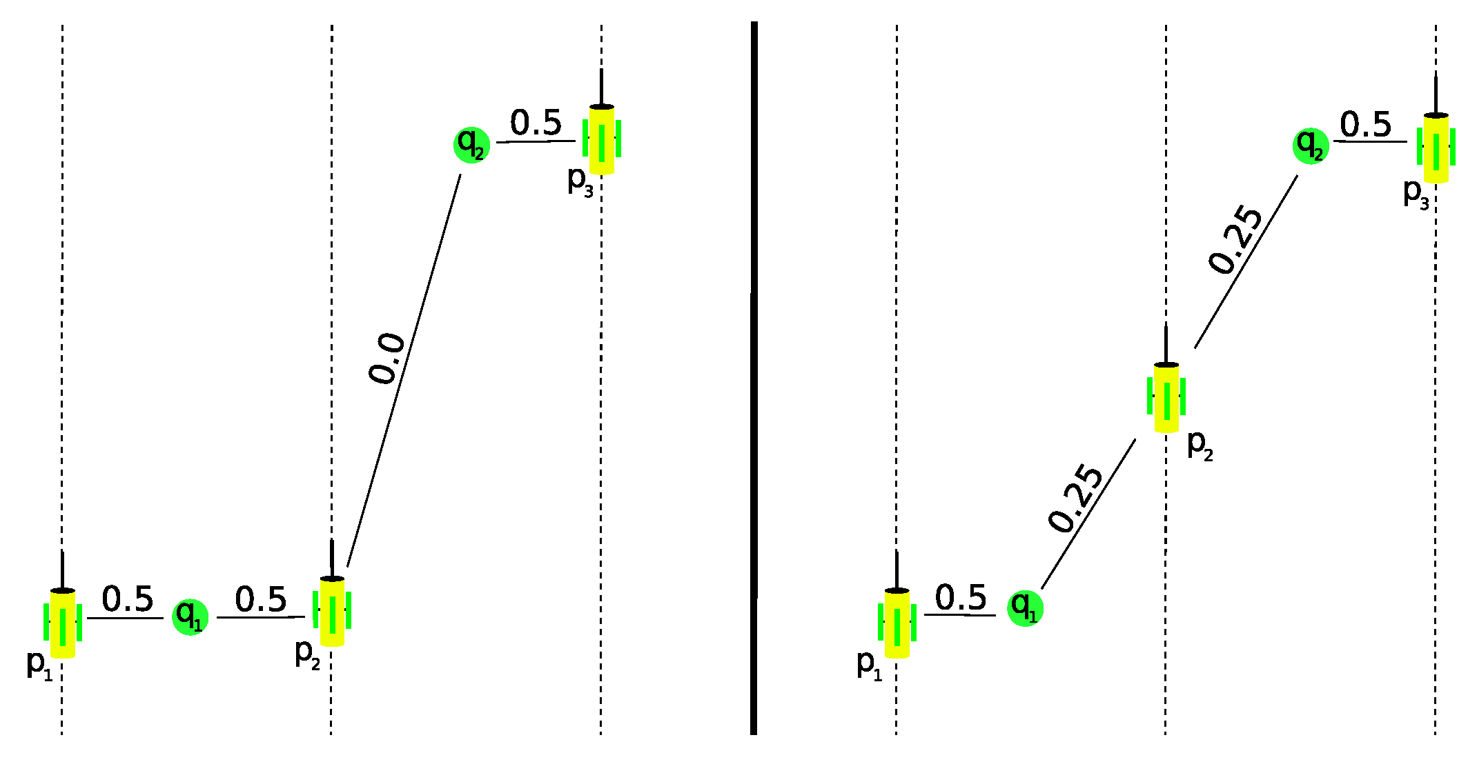
Figure 3 shows the case with three sensors,
,
and
, covering two points,
and
. For this example we assume that
and
are fixed and look at the effect of moving
. Both configurations in
Figure 3 yield an objective function value of
. This contradicts the intuition that the configuration on the right is better.
Figure 3.
Dashed lines are the motion constraints on the AquaNode motion and green circles are the points of sensor interest. Solid lines and the labels indicate the covariance between the point of interest and the indicated sensor.
Figure 3.
Dashed lines are the motion constraints on the AquaNode motion and green circles are the points of sensor interest. Solid lines and the labels indicate the covariance between the point of interest and the indicated sensor.
To prevent the problems associated with Equation (
2) and illustrated in
Figure 3, we need to ensure that the objective function penalizes regions that are already covered by other nodes. We achieve this by modifying the objective function to minimize:
Instead of maximizing the double sum of the covariance, this objective function minimizes the sum of the inverse of the sum of covariance. This reduces the increase in the sensing quality achieved when additional nodes move to cover an already covered region.
This changes the example at left in
Figure 3 to give an objective value of
. It changes the right side in
Figure 3 to
. Our new minimization of the objective function will select the rightmost configuration in
Figure 3, which is intuitively better.
To extend this to optimize placement for sensing every point in the region, we modify the objective function to integrate over all points
q in the region
Q of interest:
4.2. Objective Function
The objective function,
, is the cost of sensing at point
q given sensors placed at positions
. For
N sensors, we define the sensing cost at a point
q as:
This is the inside of Equation (
4), when
.
Integrating the objective function over the region of interest gives the total cost function. We call this function
and formally define it as:
where
Q is the region of interest. The sum over the function
is a term added to prevent sensors from trying to move outside of the water column. We need this restriction on the node’s movement to prove convergence of the controller for this cost function. Specifically, we define
as:
where
is the depth at the location
and
β is even and positive. The
component causes the cost function to be very large if a sensor is placed outside of the water column.
4.3. General Decentralized Controller
Given the objective function in Equation (
6), we wish to derive a decentralized control algorithm that will move all nodes to optimal locations making use of local information only. We derive a gradient descent controller that is localized, efficient, and provably convergent.
Our goal is to minimize
, henceforth referred to as
. To do this we start by taking the gradient of
with respect to each of the
s:
Next, we take the partial derivative of
and find:
To minimize
we move each sensor in the direction of the negative gradient. Let
be the control input to sensor
i. Then the control input for each sensor is:
where
k is some scalar constant. This provides a general controller usable for any sensing function,
. To use this controller we next present a practical function for
.
4.4. Gaussian Sensing Function
We use the covariance between points
and
q as the sensing function:
In an ideal case we would know exactly the covariance between the
sensor and each point of interest,
q. As this is not possible, we have chosen to use a multivariate Gaussian as a first-approach approximation of the sensing quality function. Using a Gaussian to estimate the covariance between points in underwater systems is common in objective analysis [
2]. In
Section 6.2 we show how to numerically estimate the covariance given real or modeled data.
We define the Gaussian to have different variances for depth () and for surface distance (). This captures the idea that quantities of interest (e.g., algae blooms) in the oceans or rivers tend to be stratified in layers with higher concentrations at certain depths. Thus, the sensor reading at a position and depth d is likely to be similar to the reading at position q if it is also at depth d. However, sensor readings are less likely to be correlated between two points at different depths. Thus, the covariance function is a three-dimensional Gaussian, which has one variance based on the surface distance and another based on the difference in the depth between the two points.
Let
be the sensing function where the sensor is located at point
and the point of interest is
. Define
to be the variance in the direction of depth and
to be the variance in the sensing quality based on the surface distance. We then write our sensing function as:
where
A is a constant related to the two variances, which can be set to 1 for simplicity.
4.5. Gaussian-Based Decentralized Controller
We take the partial derivative of the sensing function from Equation (
13) to complete the gradient of our objective function shown in Equation (9). The gradient of the sensing function
is:
Substituting this into Equation (9), we get the objective function:
4.6. Controller Convergence
To prove that our gradient controller (Equation (
11)) converges to a critical point of
, we must show [
22,
23,
24]:
must be differentiable;
must be locally Lipschitz;
must have a lower bound;
must be radially unbounded or the trajectories of the system must be bounded.
While this assures convergence to a critical point of
, small perturbations to the system will cause the gradient controller to converge to a local minimum and not an undesirable local maximum or saddle point of the cost function [
24].
Theorem 1. The controller converges to a critical point of .
In other words, as time t progresses, the output of the controller will go to zero: Proof. We show that the objective function satisfies the conditions outlined above. In
Section 4.5 we determined the gradient of
, satisfying condition 1.
has a locally bounded slope, meaning it is locally Lipschitz and satisfies condition 2.
To show that
is bounded below, to satisfy condition 3, consider the composition of the objective function:
The
term is the sum of a number raised to an even power and is clearly bounded below by zero. Expanding the notation in the integral term we can see:
and
is a Gaussian, which is always positive. The integral and sum of positive terms is also positive. Thus, both terms and therefore
are bounded below by zero, satisfying condition 3.
Unfortunately,
is not radially unbounded. However, the trajectories of the system are bounded, satisfying condition 4. To see this, note that the trajectories of our system are along the
z-axis. Equation (
7) defines the
term. By choosing a sufficiently large
β, the cost of moving outside of the column overcomes any potential sensing advantage gained by moving outside, as the integral term of
is bounded below.
Thus, we have satisfied all the conditions for controller convergence, proving that our controller converges.
5. Collaborating with Underwater Robots
The depth adjustment system on the AquaNodes makes them very versatile for sampling the full water column; however, their translational position cannot be easily changed. In this section, we adapt our decentralized control algorithm to allow the sensor network to tell the robot the best path to traverse while also adapting the positions of the underwater sensor nodes.
We desire a decentralized approach where each node along the robot’s path informs the robot of the next part of the path. This is important to ensure that the network does not need to transmit all information to the robot before the robot starts. In addition, this lets the network reconfigure to new depths before the robot enters the system to enable collection of data from locations of highest utility at the same time. This would not be possible if, for instance, the robot communicated with local nodes and decided its trajectory online.
5.1. Problem Formulation
In order to allow the underwater sensor network to compute the best path for the robot, we start by extending our basic controller described by Equation (
6) to include sensing locations along the robot’s path,
:
Note we drop the
ϕ term from Equation (
6) for simplicity of notation. We use the superscript
to indicate that this is a sensing location along the robot’s path. We choose these as points evenly spaced between the locations of the static sensor nodes. There can be as many points along the robot’s path as needed, although in practice we use just a few intermediate points between static sensors as discussed in
Section 6.6 to minimize path complexity. The controller then adjusts the depth of this robot sensing point while keeping
fixed.
This controller works to optimize the sensing with all of the sensor node locations and all of the robot sampling points. However, this could result in paths where the robot alternates moving between the surface and bottom of the water column. This is costly in terms of traversal time and does not take advantage of the sensor nodes that can cover the extreme depths more easily than the robot. To reduce the length of the path the robot travels, we introduce an additional term that aims to minimize the length of the path that the robot traverses. We call this
and define it as:
where
is the Euclidean distance between the two points
and
.
5.2. Robot-Sensor Node Decentralized Controller
We now combine
and
to create a new objective function that we will use as part of our new decentralized controller that controls the robot path and the sensor node locations. We call this controller
and define it as:
The term
is a weighting term between the first component that optimizes the positions for sensing and the second term that minimizes the path length the robot travels. We investigate the sensitivity of the algorithm to different values of
α in
Section 6.6. As in
Section 4.5, we develop a decentralized controller by taking the gradient of
with respect to changes in depth and move each sensor node and robot sensing location by
. For space considerations we omit the details in this section, but note that the controller derivation and convergence proof closely follow that of the controller solely for sensor node. Each sensor node is responsible for computing and updating the robot sensing locations
that are closest to it. When the robot comes into the communication range of a node, it will transmit the next sensing locations to the robot.
In practice, the sensor network may have a schedule of times when the robot will enter the network, or alternatively, the robot will inform nearby nodes when it enters the network. These nodes will then start running the depth adjustment algorithm to compute the best path for the robot and any corresponding changes in the depths for the sensor nodes. This will propagate through the network, and as the robot moves, it will receive updated way points from nearby sensor nodes.
6. Simulation Experiments
In this section, we discuss the results of simulation experiments that test the performance of the algorithm. In addition, we analyze the sensitivity of the algorithm to different parameters that could impact the algorithm on real hardware (
Section 7 covers experiments on the hardware platform). We start by looking at the base algorithm without a mobile robot and then introduce the robot into the system. Before that, we first detail our implementation and discuss how we determine the covariance model.
6.1. Implementation
Algorithm 1 shows the implementation of the decentralized depth controller (Equation (
8)) in pseudo-code. This is the implementation we use in our simulations and on the hardware platform. On our hardware platform this algorithm runs in real-time. The procedure receives as input the depths of all other nodes in communication range. The procedure requires two functions
F(p_i,x,y,z) and
FDz(p_i,x,y,z). These functions take the sensor location
and the point
that we want to cover. The first function,
F(p_i,x,y,z), computes the covariance between the sensor location and the point of interest. The second function,
FDz(p_i,x,y,z), computes the gradient of the covariance function with respect to
z at the same pair of points.
After the procedure computes the numeric integral, it computes the change in the desired depth. This change is bounded by the maximum speed the node can travel. Finally, the procedure changes the node depth. Note that for this implementation we ignore the impact of (from Equation (9)) on the controller. Instead, changeDepth puts a hard limit on the range of the nodes, preventing them from moving out of the water column. We found that this had little impact on the results.
| Algorithm 1 Decentralized Depth Controller |
1: procedure updateDepth()
2:
3: for to do
4: for to do
5: for to do
6:
7: for to N do
8: F(p_i,x,y,z)
9: end for
10: FDz(p_i,x,y,z)
11: end for
12: end for
13: end for
14:
15: if then
16:
17: end if
18: if then
19:
20: end if
21: changeDepth(delta)
22: end procedure
|
Algorithm 2 shows the algorithm implementation when there is also a robot in the system, as described in
Section 5. This algorithm is run for both sensor node locations and for the robot sensing locations. There are two key changes in this algorithm. Line 11 adds the sensing contribution from the robot sensing locations. This is applied both when computing the control for the sensor nodes and for the robot sensing locations. Line 18 is added only when control is being calculated for the robot sensing locations. This adds in the component of the controller related to the distance between robot waypoints.
6.2. Covariance Model
In
Section 4 we developed the decentralized depth controller algorithm using a multivariate Gaussian as the covariance function. However, more generally, if we have real information about the system, we can numerically compute the covariance. Since we are interested in the Neponset River, in this section we show how we compute a covariance model based on model data.
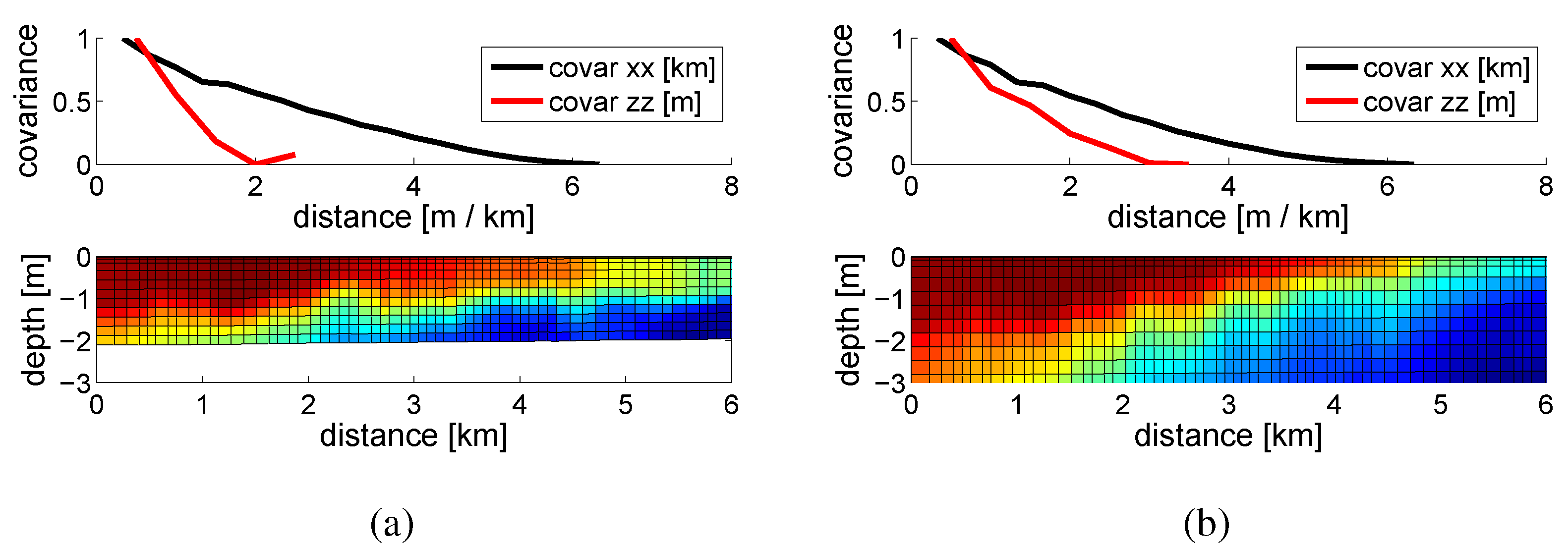
Figure 4 (bottom) shows the concentration of CDOM in the Neponset River, which feeds into Boston Harbor at two different tide levels. We find that the CDOM concentration is highly dependent on the tide level. Other parameters that may impact CDOM concentration include rainfall and wind patterns. This data was computed from a numerical model for Boston Harbor as described in
Section 3. The model is accurate on average; however, new measurements from the A
quaN
odes will be used to further refine and calibrate the Neponset River and Boston Harbor models.
| Algorithm 2 Decentralized Depth Controller with Robot Sensing |
1: procedure updateDepth(, )
2:
3: for to do
4: for to do
5: for to do
6:
7: for to N do
8: F(p_i,x,y,z)
9: end for
10: for to M do
11: F^R(p_i,x,y,z)
12: end for
13: FDz(p_i,x,y,z)
14: end for
15: end for
16: end for
17: if RobotWaypoint then
18:
19: end if
20:
21: if then
22:
23: end if
24: if then
25:
26: end if
27: changeDepth(delta)
28: end procedure
|
Figure 4.
(Bottom) Model of the CDOM concentration in the Neponset river when tide caused a river depth of on average 2 m (a) and 3 m (b). (Top) The corresponding numerically computed covariance.
Figure 4.
(Bottom) Model of the CDOM concentration in the Neponset river when tide caused a river depth of on average 2 m (a) and 3 m (b). (Top) The corresponding numerically computed covariance.
Figure 4 (top) shows the numerically computed covariance along the length of the river and depth. We numerically computed the covariance along the length of the river by examining each pair of points at distance
k apart and taking the sample covariance, which is
for the N points
a and
b that are
k distance apart. We compute the covariance along the depth of the river in a similar manner.
Most of the sensors we use only measure the value at the location of the sensor node. Using covariance allows us to expand the range of the sensor by determining the likely relation between the location of the sensor and other locations. This can fail in some situations where there are discontinuities in the sensory field, for instance strong currents bringing in different water. However, the covariance function can be adjusted to take into account this type of geographic dependence if these types of discontinuities are expected or detected.
We fit a Gaussian basis function to the numeric covariance curve. To do this we use MATLAB’s
newrb function.
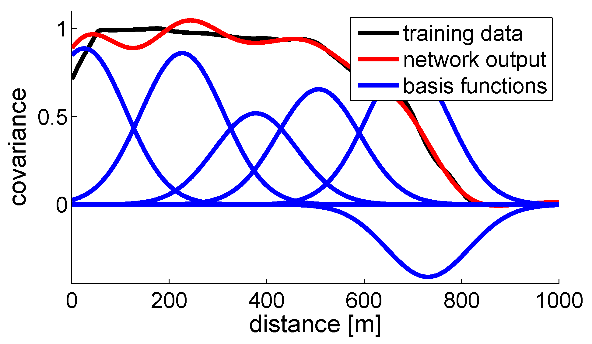
Figure 5 shows the result of the basis function fit. The error in the fit depends on the number of Gaussians used. For this plot with 6 elements the error is 1.88%, whereas using 10 elements gives an error of 0.54%. Using a basis function gives us a compact representation of the covariance function that a sensor node can easily store and compute.
An advantage of using a Gaussian basis function is that it allows online updates of the covariance function based on the sensed data. Nodes can share and learn the parameters of the basis function using a number of existing techniques for fitting basis functions to unknown data [
25].
Figure 4 shows two different tide levels in the river system. Different covariance functions, based on the tide, enable dynamic repositioning of the sensor network to adapt to changing conditions.
Section 7.2 discusses changing covariance functions to account for tidal changes in a river.
Figure 5.
The Gaussian basis function elements for a fit with 6 basis functions.
Figure 5.
The Gaussian basis function elements for a fit with 6 basis functions.
6.3. Simulation Parameters
We implemented the decentralized depth controller with the Neponset covariance model in MATLAB to test the performance of Algorithm 1. In these experiments, unless otherwise noted, we use a “k” value of 0.001, capped with a maximum speed of ±2
. Each node performs twenty iterations of the controller. The nodes are placed in a line spaced 15 m apart from each other and are in “water” of 30 m depth with a starting depth of 10 m. A 1 m grid is used to integrate over for all operations. We do not consider the impact of the robot until
Section 6.6.
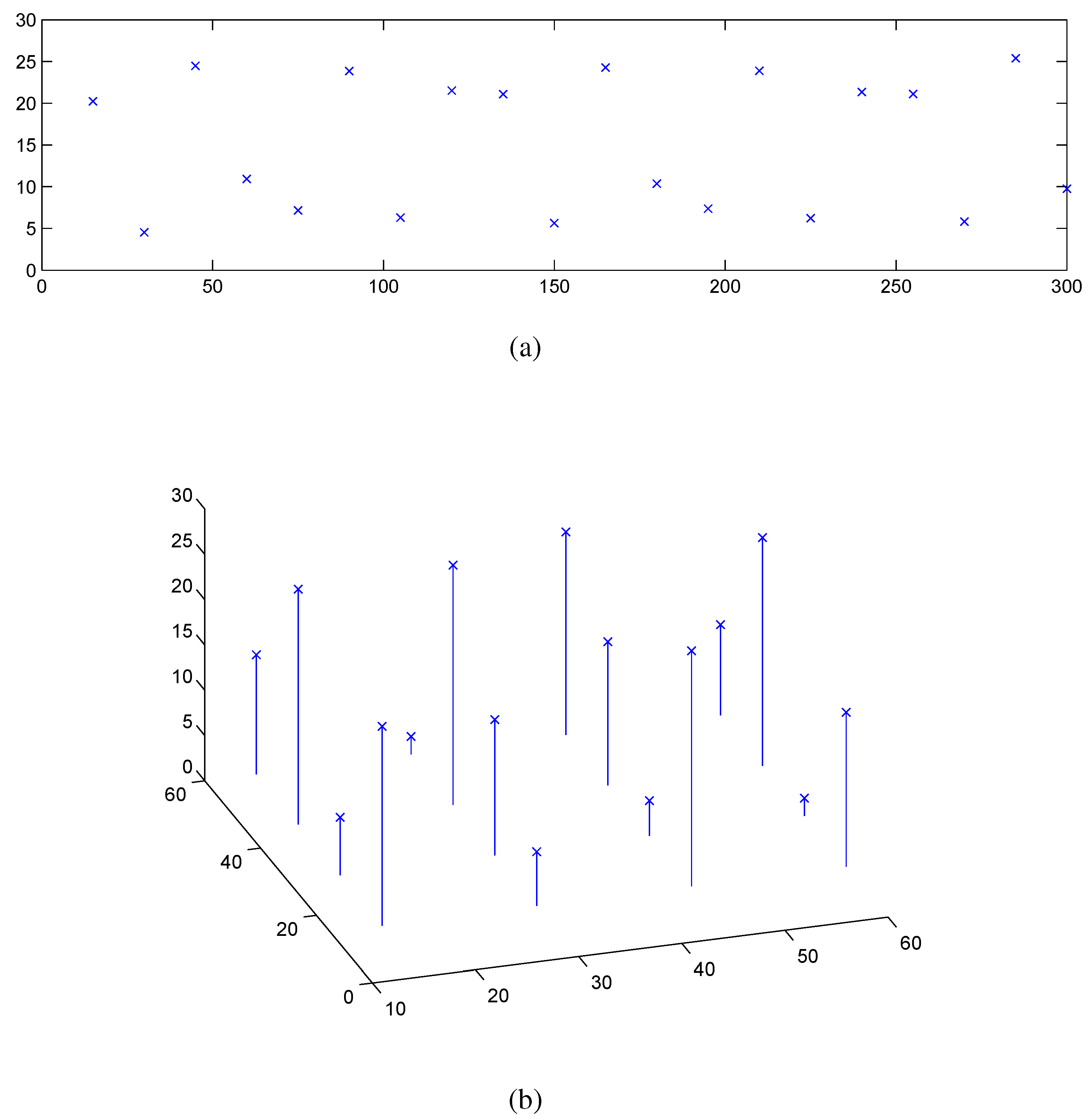
Figure 6a shows the results after running the decentralized controller on a network of 20 nodes. Each iteration of the algorithm took 8 s per node with convergence occurring after 6 iterations.
Figure 6b shows the result of an experiment with 16 nodes arranged in a 4-by-4 grid with 15 m spacing in 30 m depth. Each iteration of the algorithm took 2 min per node with convergence occurring after 7 iterations. We now explore the sensitivity of the algorithm to different parameters.
Figure 6.
The final positions after the distributed controller converges for a (a) 2D and (b) 3D setup.
Figure 6.
The final positions after the distributed controller converges for a (a) 2D and (b) 3D setup.
6.3.1. Changing k
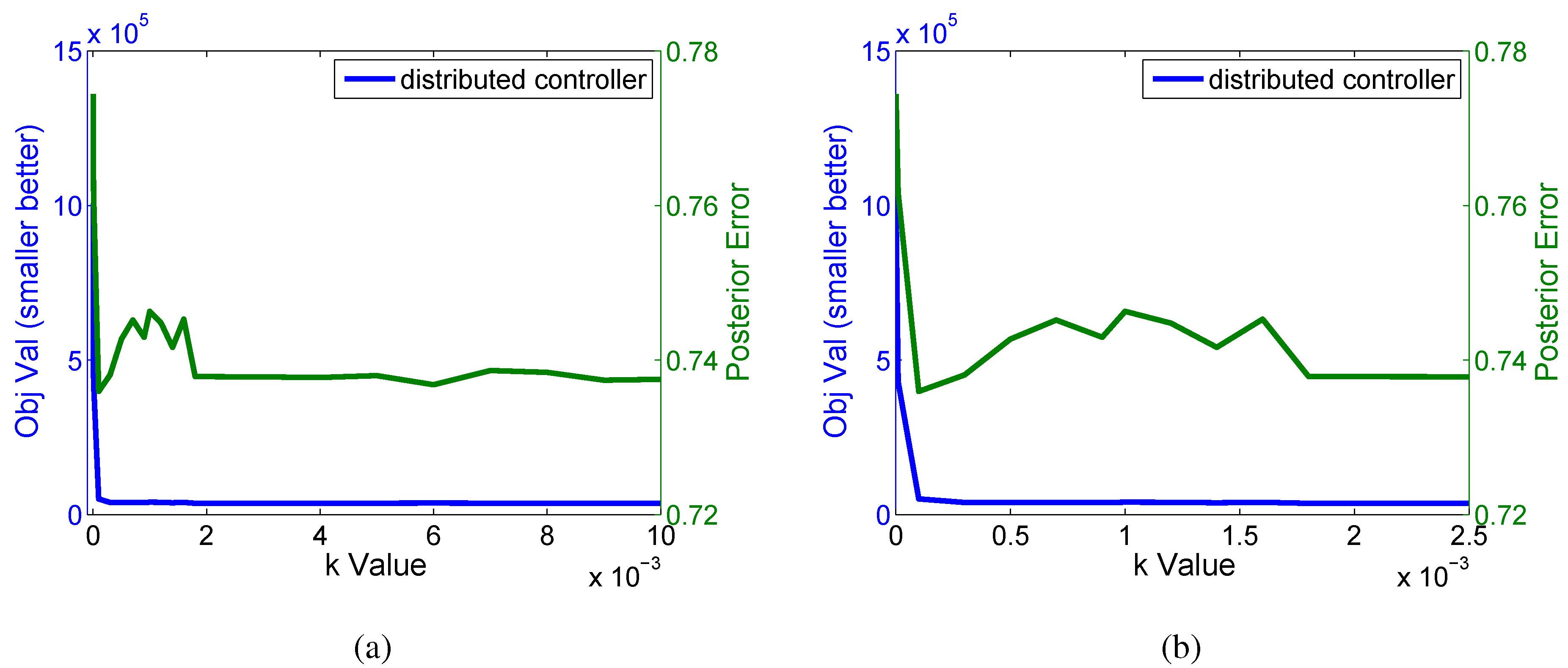
Figure 7 shows the effect of changing the
k value on the objective value
for a system with 20 nodes. Recall that each node moves according to:
Increasing the value of k causes the nodes to move down the gradient of more quickly. Values that are too large can lead to oscillations around the final configuration or lead to instabilities in the system. If the value of k is too small, the system may not move fast enough to converge within a reasonable number of steps.
Figure 7.
The objective value and posterior error found when different “k” values are used in a system with 20 nodes. Inset (a) shows the full range of values explored. Inset (b) shows a zoomed in section of (a) to highlight the area where values of “k” can produce some instabilities.
Figure 7.
The objective value and posterior error found when different “k” values are used in a system with 20 nodes. Inset (a) shows the full range of values explored. Inset (b) shows a zoomed in section of (a) to highlight the area where values of “k” can produce some instabilities.
Figure 7a shows the range of
k’s explored, while
Figure 7b zooms in on
k values less than
. Using a
k value of less than
yields very poor results, since the system does not converge within the 20 iterations of the algorithm that we allow. For values of
k between 0.0001 and 0.002 the objective value converges and is better, but the posterior error is not stable, showing that the positions are still not as good as with larger
k within the 20 iterations.
For values of
k over
, we see in
Figure 7 that it performs well. While we would expect to see oscillations as
k increases, we do not see so since the maximum speed that the nodes can travel is limited to 2 m/s. Therefore, in practice the value of
k matters little as long as it is sufficiently large. However, we should warn readers that oscillations may occur in different systems with faster maximum speeds.
6.3.2. Changing Neighborhood Size
We examine the effect of changing the neighborhood size. The neighborhood size is the size over which each node integrates when computing the numeric integral (Algorithm 1, line 10). The decentralized controller assumes that it has information about the depths of all nodes in the system. In practice we can only know the depths of our neighbor nodes due to poor acoustic communication. The covariance function decays rapidly with distance, reducing the effect of far away sensors, allowing nodes to ignore the sensors they cannot hear. This means that multi-hop messaging is not needed to communicate information for the depth controller, enabling very large deployments without communication overhead.
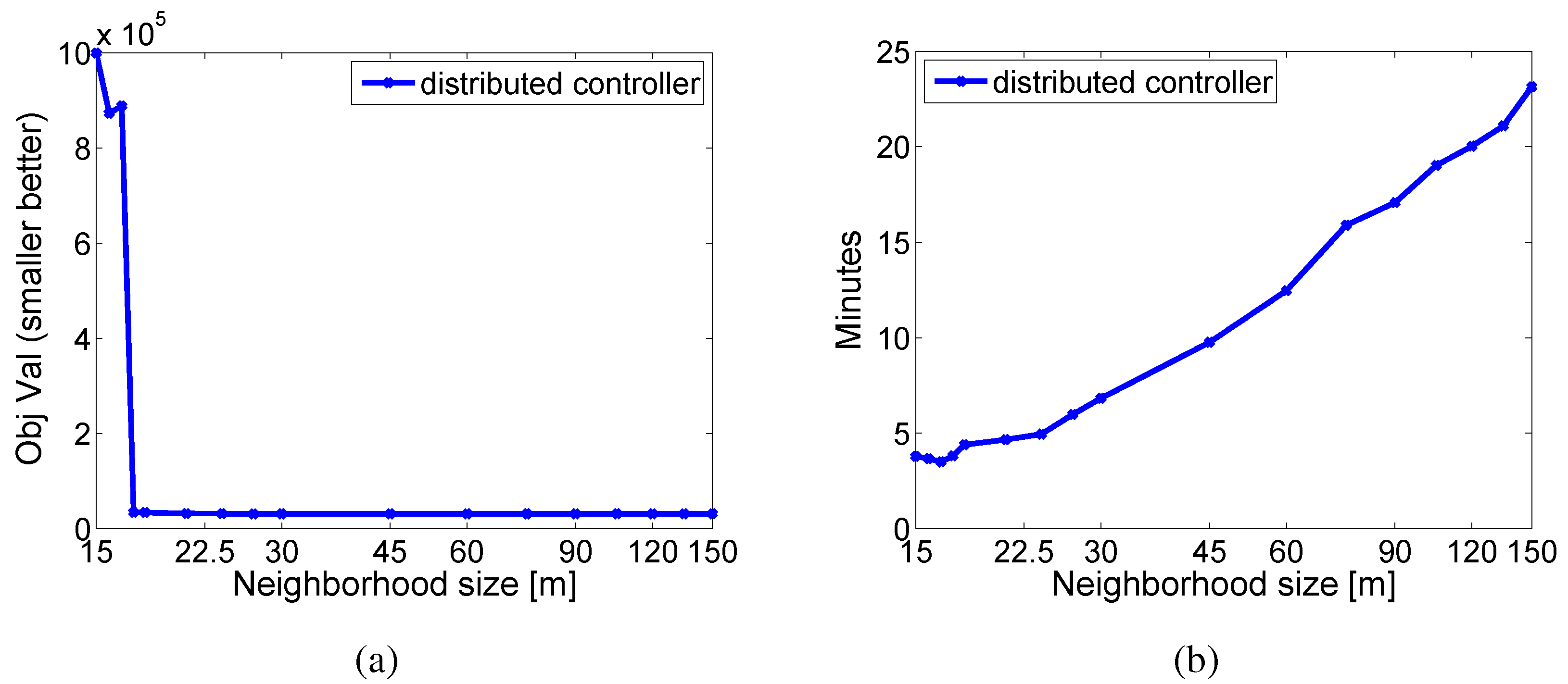
Figure 8 shows the results of changing the size of the neighborhood over which we integrate. For this simulation the nodes were placed 15 m apart. The neighborhood size varied from ±15 m to ±150 m. As can be seen from
Figure 8a, using a neighborhood of just 15 m results in very poor performance. However, a slight increase in neighborhood size drastically increases performance. This indicates that the near neighbors have the largest impact. Thus, the neighborhood size should be chosen to include all one-hop neighbors.
Figure 8b shows that the total runtime required for the algorithm increases in a linear fashion as the neighborhood size increases. This experiment verifies the intuition that nodes only need to hear direct neighbors to have good performance.
Figure 8.
The (a) objective value and (b) runtime for a 15 node network when changing the size of the neighborhood over which the integration occurs.
Figure 8.
The (a) objective value and (b) runtime for a 15 node network when changing the size of the neighborhood over which the integration occurs.
6.3.3. Changing Grid Size
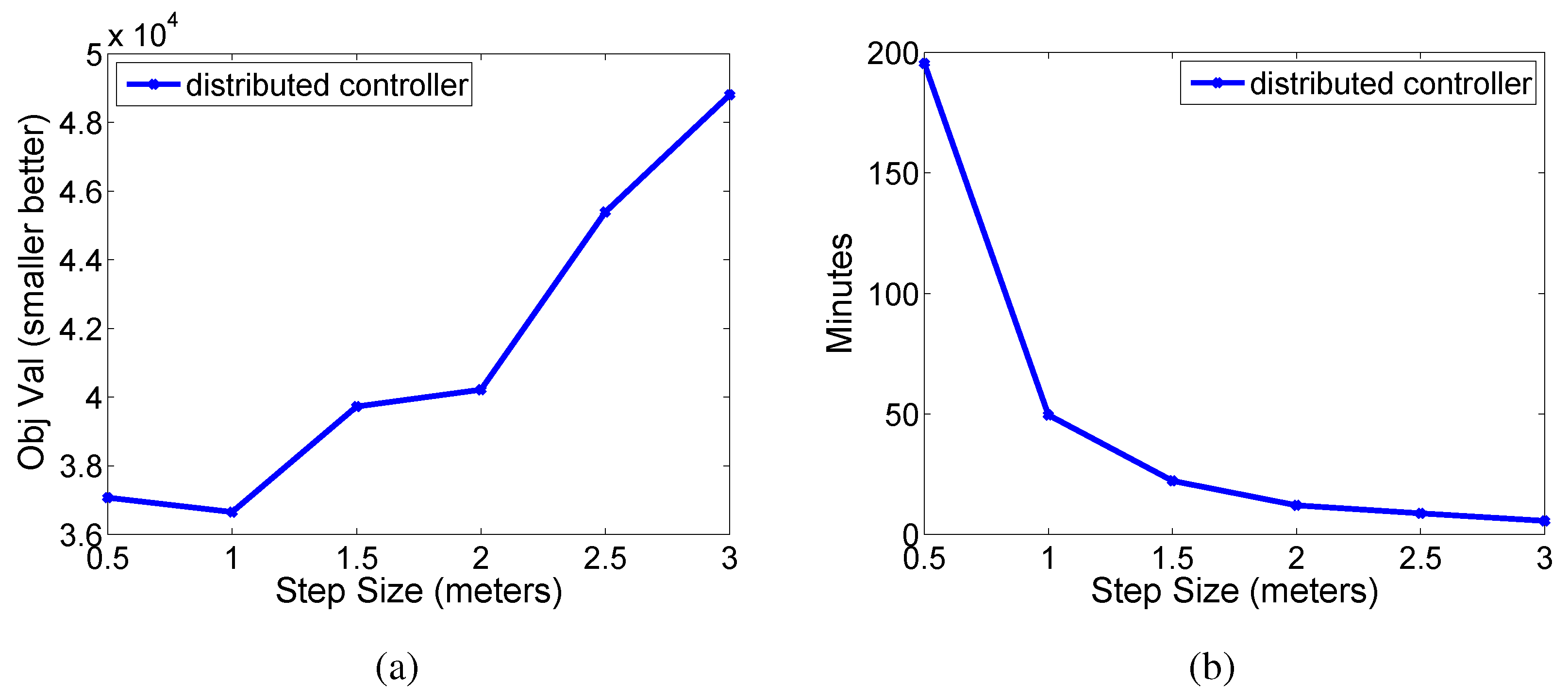
We examine the impact of changing the size of the grid over which we numerically integrate. In simulation we uniformly change the step size in the x and z axes. Using a large step size reduces the computations needed to perform the decentralized controller; however, if the step size is too large, important regions may be overlooked, causing degradation in performance.
Analyzing Algorithm 1 we see a runtime of
, where
represents the number of steps in the grid along the
x-axis and
N is the number of sensor nodes in the system. As shown in
Figure 9b, the runtime decreases in a quadratic fashion as the step size increases. The quadratic results from the 2D simulation; in the 3D case the runtime would decrease cubically as the step size increases.
Figure 9.
Changing the grid size. (a) Objective value and (b) total search time as the step size changes.
Figure 9.
Changing the grid size. (a) Objective value and (b) total search time as the step size changes.
Figure 9a shows the impact of changing the grid size on the objective function. As step size increases, the objective function increases as well. Thus, a grid size of 1 m seems reasonable, because it is the minimum grid size and results in a good runtime. If the spacing of the nodes was closer, a finer grid may be needed, and similarly, if they are spaced further apart, a larger grid could be used. In our experience having between ten and twenty steps between each pair of nodes yields a good balance between runtime and algorithm performance.
6.3.4. Changing Start Configurations
In the prior sections we started the A
quaN
odes in a straight line configuration before running the decentralized controller. We now examine how close the decentralized controller comes to obtaining the global minimum of the system with different start configurations.
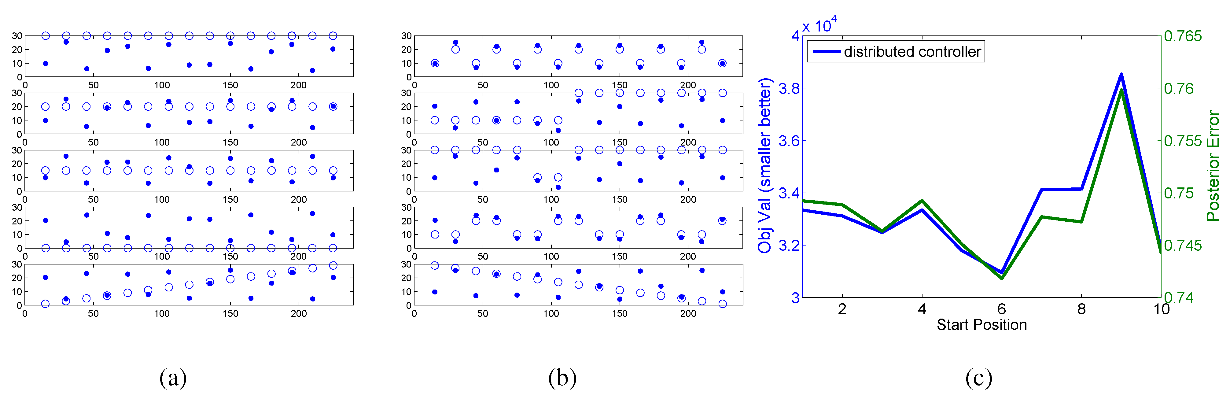
Figure 10a,b shows the various starting and ending configurations, and
Figure 10c shows the final objective value and posterior error for these trials.
We tested a number of start configurations. In all of these experiments the final configuration ended up with nodes roughly alternating. However, some local minima occur that result in a worse objective function value. In particular, the second last configuration in
Figure 10b, which alternated two nodes down and two nodes up, resulted in a similar final configuration. As can be seen in
Figure 10c, this configuration yielded the worst objective value and posterior error of all the trials.
Figure 10.
(a,b) The results of the running the depth adjustment algorithm on various node start positions (circles) and (c) the resultant objective value and posterior error.
Figure 10.
(a,b) The results of the running the depth adjustment algorithm on various node start positions (circles) and (c) the resultant objective value and posterior error.
We can contrast this with the configuration in
Figure 10b (top), which resulted in the best objective value. The remainder of the configurations fell somewhere in between these two. Some configurations demonstrate that a local minimum can occur that is hard to overcome. Fortunately, although this occurs occasionally, it is not often, and when it does occur the system still obtains fairly good results. It is possible to avoid local minima by starting with configurations that are known to be near-optimal (for example, up-down-up configurations). In addition, in situations where the covariance function is periodically updated, the nodes can return to a near-optimal configuration before performing the update.
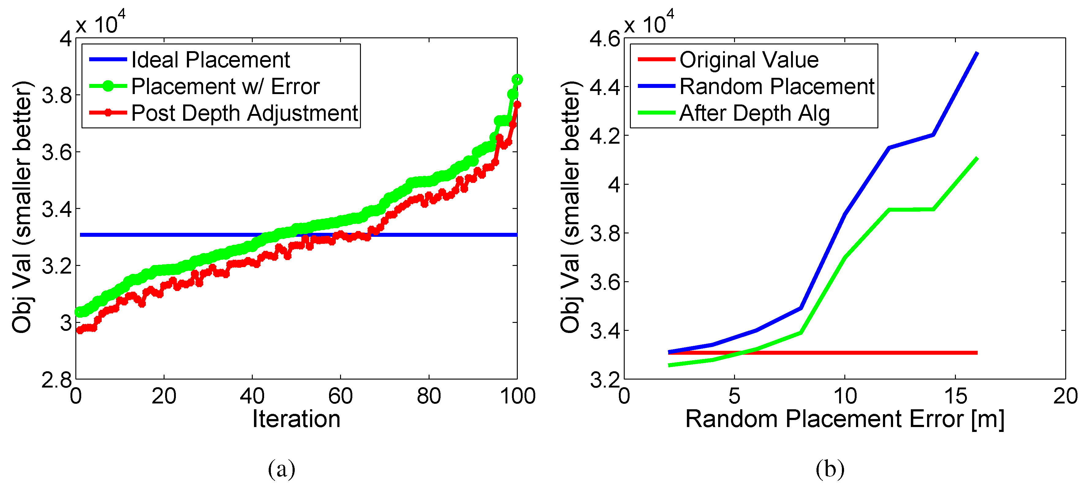
6.3.5. Random Placement Error
As it is impossible to perfectly place nodes in a real-world setup, we examine the effects of random variation in the
x-axis placement of the nodes. The nodes were deployed starting in the ideal depth configuration.
Figure 11a demonstrates the results of 100 trials with ±6 m random error added to the ideal node positions in the
x-axis. The 100 trials are sorted by the objective function in the plot. We then run the depth adjustment algorithm on the misplaced nodes, which improves their overall depth positioning for sensing.
Figure 11b outlines this for errors in
x-axis placement ranging from 2 m to 16 m. Each point is the average of 100 random trials. Again the depth adjustment algorithm improves the overall position. This experiment shows that the decentralized depth adjustment algorithm can improve the overall sensing even if the start depths (
z-axis) are ideal and the
x-axis placement is not.
Figure 11.
Nodes deployed with random error in x-axis placement. (a) Plot of 100 runs with 6 m error. (b) Average over many runs and positions.
Figure 11.
Nodes deployed with random error in x-axis placement. (a) Plot of 100 runs with 6 m error. (b) Average over many runs and positions.
6.4. Data Reconstruction
The ultimate goal of placing sensors is reconstructing the complete data field, not just the points where sensors exist. The distributed depth adjustment algorithm places sensors in locations to maximize the utility of the sensed value for doing this type of reconstruction. In this section we show the results of simulations in reconstructing data fields given point measurements at sensor node locations.
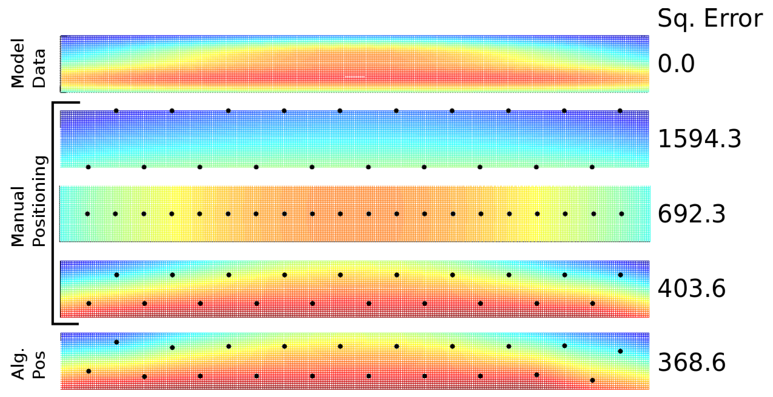
Figure 12 shows the results of reconstructing a field given three manually configured sensor placements and the depth adjustment algorithm. At the top in
Figure 12 we show the actual field we attempt to recover. This field is a semi-randomly chosen field that has similar covariance properties to the Gaussian covariance. The manually chosen configurations were: (1) sensors placed alternatively at the top and bottom of the water column; (2) sensors placed in the middle of the water column; (3) sensors placed a quarter of the way off the top and bottom. Finally, at the bottom is the positioning based on the depth adjustment algorithm. While visually similar to the manually chosen configurations, it slightly improves upon the positions to better cover the region.
To quantify this we use the sum of squared error metric, comparing the actual model data to the recovered using MATLAB’s “v4” version of
griddata. The sum of squared error values are shown in the right of
Figure 12. The dynamic depth adjustment algorithm outperforms the three manually chosen configurations.
Figure 12.
From top: model data, reconstructed data for three manual configurations, and for algorithm positioning.
Figure 12.
From top: model data, reconstructed data for three manual configurations, and for algorithm positioning.
6.5. Comparison with Posterior Error
A common metric for defining how an area is covered by sensors is to examine the posterior error of the system [
26]. Calculating the posterior error requires that the system can be modeled as a Gaussian process. This is a fairly general model and valid in many setups. The posterior error of a point can be calculated as:
The vector is the vector of covariances between q and the sensor node positions . The vector is transposed. The matrix is the covariance matrix for the sensor node positions. The values of are for each entry .
Figure 13.
Posterior error.
Figure 13.
Posterior error.
This computation, however, requires an inversion of the full covariance matrix. This is impractical on real sensor network hardware that has limited computation power and memory. As such, we cannot calculate the posterior error on the sensor nodes, but we can calculate it as a metric to evaluate our own objective function and compare different sensing configurations. As shown in
Figure 10c, the posterior error and the objective function track each other, showing that our metric has similar properties to that of the posterior error metric.
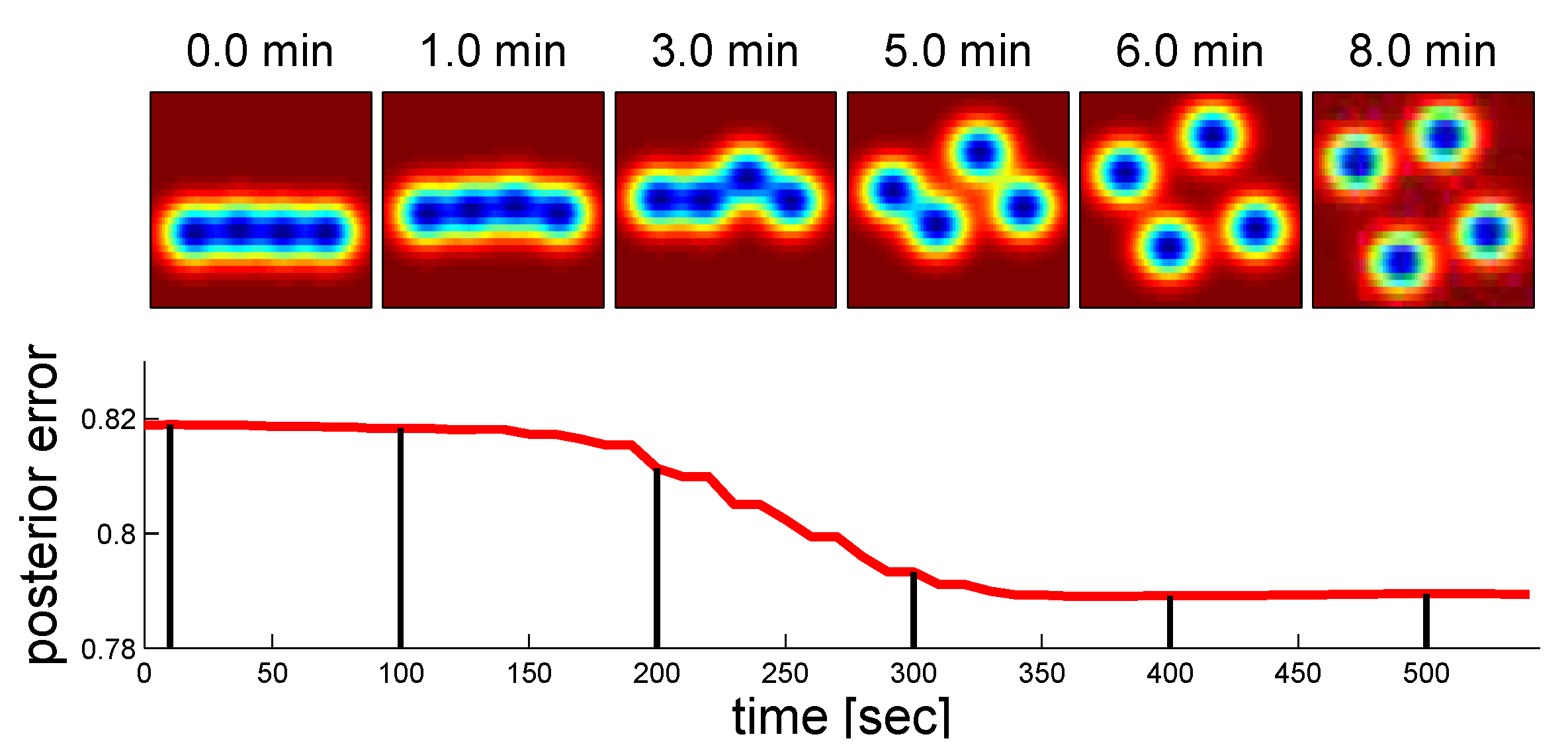
Figure 13 (bottom) shows a plot of a run of the decentralized depth controller and plots the normalized sum of the posterior error at all points.
Figure 13 (top) shows snapshots of the plots of the posterior error as the algorithm progresses. The algorithm performs well under this metric as well as the objective function metric.
6.6. Mobile Robot
We now examine the performance of Algorithm 2, which includes computing the robot path.
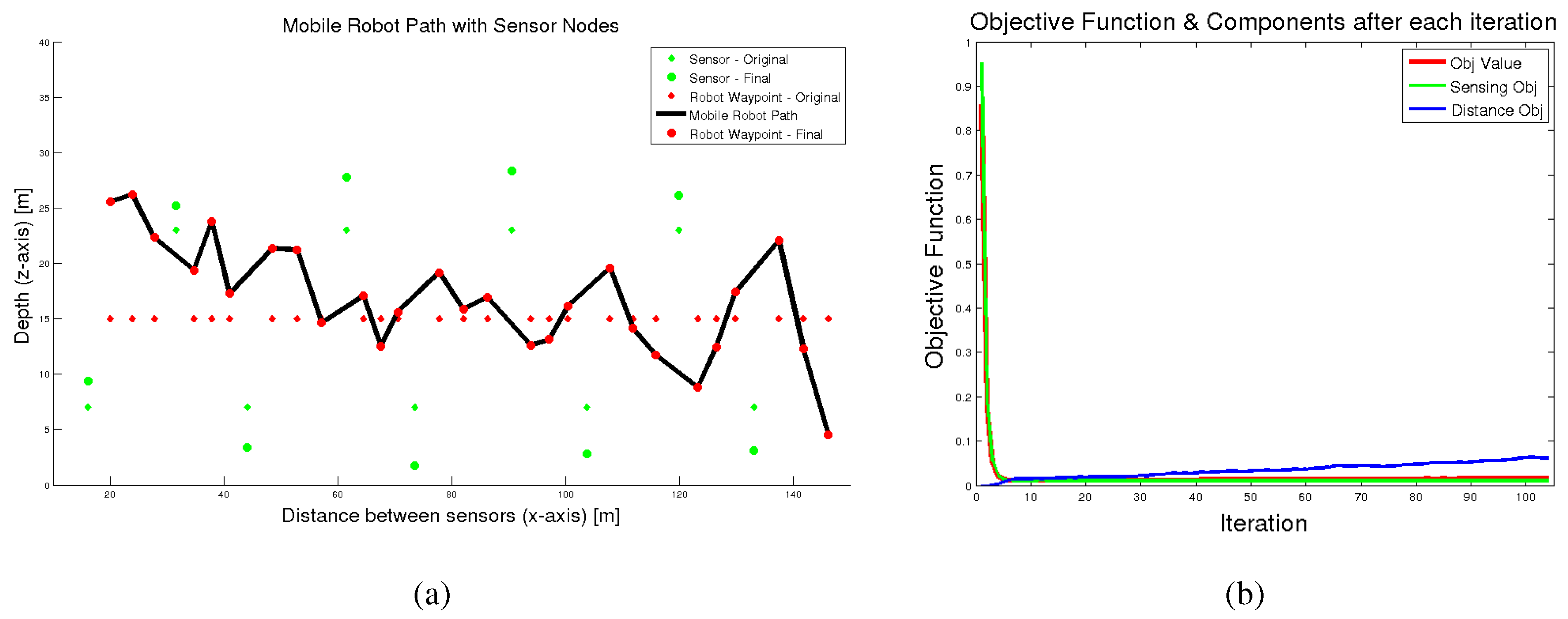
Figure 14a shows the initial and final configurations of the underwater sensor nodes and robot path points, and
Figure 14b shows the objective functions. We started with the nodes in alternating configurations, as is typical after running the depth adjustment algorithm with the sensor nodes alone. Between each sensor node, we created 3 waypoints at a mid-level depth. Each sensor nodes is responsible for optimizing the position of the robot path waypoints that are closest to its position. For this experiment we used an
α value of 0.1, which puts more weight on optimizing sensing.
Figure 14.
Example showing how the (a) sensor nodes move to accommodate the robot and (b) the corresponding objective functions (normalized).
Figure 14.
Example showing how the (a) sensor nodes move to accommodate the robot and (b) the corresponding objective functions (normalized).
Figure 14a shows that after running the algorithm the underwater sensor nodes spread further apart. This happened since the robot covers much of the central area of the water, allowing the sensor nodes to cover more at closer to the surface and bottom. The robot path tends to alternate up and down in an opposite zigzag from the positions of the underwater sensors. This allows it to cover more area sensing. Also note that on the far left of the figure the robot is high in the water to cover an area where there is no nearby sensor and a similar configuration happens on the right side of this figure. In this figure, the robot path shows some relatively large changes in depths at some locations (e.g., around 40 m).
Figure 14b shows the normalized overall objective function over the algorithm iterations and also the individual components that make up the sensing objective function and distance objective function. Recall from Equation (
21) that these are weighted by the parameter
. This figure shows that the sensing objective function and overall objective function rapidly decrease. The distance function, however, slowly increases for a time until it stabilizes. This shows that the robot path length is increasing to improve the overall sensing quality.
The maximum amount that the path length will increase to improve the path for sensing is controlled by the weight parameter
α. Recall from
Section 5 that
α in essence controls the length of the robot path. A high alpha will shorten the robot path, while a lower alpha will result in a longer path but better sensing.
Figure 15 shows the maximum path length for different values of
α. For
the path length is nearly the minimal possible, indicating for these values the robot basically follows a straight line. For
the path length is higher, which indicates the robot is traversing in more of a zigzag pattern. In some configurations (e.g., in deeper water), the differences between the
α values less than 0.55 is more pronounced, but in this configuration the maximum length of the path is bounded by the positions of the sensor network nodes.
Figure 15.
Alpha versus the maximum path length.
Figure 15.
Alpha versus the maximum path length.
These experiments demonstrate how Algorithm 2 functions to create a path for the robot and adjusts the depths of the underwater sensors to improve the sensing, while balancing out the maximum path length of the robot. We also showed how the choice of α impacts the overall length of the path the robot takes. This parameter can be adjusted based on the mission requirements of the robot.
7. Hardware Experiments
Figure 16 shows the underwater sensor nodes and the robot. We performed experiments in lab, pool, and rivers using four of our underwater sensor nodes equipped with the depth adjustment system. For these setups the sensor network ran the decentralized depth controller. We tested both the base covariance model discussed in
Section 4.4 and the model-based covariance discussed in
Section 6.2. We have not yet tested the controller with the robot under field conditions, but plan to do so during future field experiments.
We implemented Algorithm 1 on the AquaNodes. The algorithm runs in real-time on the AquaNode and Amour hardware, enabling adjustment of the positions and paths online. For the implementation of FDz(p_i,qx,qy,qz) (line 10) we use the numerical gradient of F at that position. We use this to avoid deriving the gradient for every covariance function. The two different covariance models require different implementations of the function F (line 8).
Figure 16.
AquaNodes and Amour.
Figure 16.
AquaNodes and Amour.
For the base covariance model discussed in
Section 4.4 we implemented the
F as:
exp(-(((px-qx)*(px-qx)+(py-qy)*(py-qy))
/(2.0*SIGMA_SURF*SIGMA_SURF)
+((pz-qz)*(pz-qz))/(2.0*SIGMA_DEPTH*SIGMA_DEPTH)));
with
SIGMA_DEPTH = 4.0 and
SIGMA_SURF = 10.0. Some additional optimizations were made to limit duplicate computations. For the algorithm, the node locations were scaled to be 15 m apart along the
x-axis, the neighborhood size was ±20 m along the
x-axis, the virtual depth ranged in
z from 0 to 30 m, and a step size of 1 m was used.
For the covariance based on the model data (CDOM covariance), we implemented
F based on the Gaussian basis function. Since we used MATLAB’s
newrb function to compute the basis function, we used their documentation to determine the reconstruction of
F:
val = 0.0; for(i = 0; i < NUM_BASIS; i++){ val += netLWX[i]
*exp(-pow(((fabs(px-qx)-netIWX[i])*netb1X[i]),2)); val += netLWZ[i]
*exp(-pow(((fabs(px-qx)-netIWZ[i])*netb1Z[i]),2));
}
val += netb2X + netb2Z; Yme = Yme + net.b{2};
The value
netLW is the amplitude and
netIW is the center of the Gaussian as reported by MATLAB. The factor
netb1 is the inverse of the variance of the Gaussian. The actual values of these variables are dependent on the model data. As discussed in
Section 6.2 and shown in
Figure 5, a Gaussian basis function produces a good fit as compared with the actual data for the Neponset River CDOM covariance. For this setup, the node locations were scaled to 500 m spacing along the
x-axis, the neighborhood size was ±800 m, the depth ranged from 0 to 3 m, the step size was 40 m along the
x-axis, and a step size of 0.1 m in depth was used.
7.1. Lab and Pool
With these two covariance models and implementations we performed experiments in lab and in pool. Both sets of experiments used four underwater sensor nodes. For the lab experiments, we placed the transducers of the acoustic modem in a bucket of water and allowed the winch system to operate freely in air. The lab experiments required the same functionality as the pool experiment while providing improved acoustic communication. For the pool experiments, we placed the four sensor nodes in a line in the deep end of a 3 m deep pool.
As the pool and bucket did not allow the node spacing used in the setup, we manually set the positions of the nodes to have the proper x-axis spacing. We also scaled each node’s estimated depth to map the range of depth used in the covariance model to a 1 m depth range in the pool. This was to keep the sensor nodes near the middle of the column of water, as the acoustic modems were not able to communicate with each other if they were outside of the range.
7.1.1. Results
We successfully ran multiple iterations of both covariance models in the bucket and the pool. For the Gaussian we ran 4 trials in the pool. The algorithm ran on the AquaNodes and allowed adjustment in real-time without any external computation. Each trial converged within 12 min with each iteration averaging 14 s. For the CDOM covariance we ran 5 pool trials. Each trial converged within 20 min with each iteration averaging 35 s.
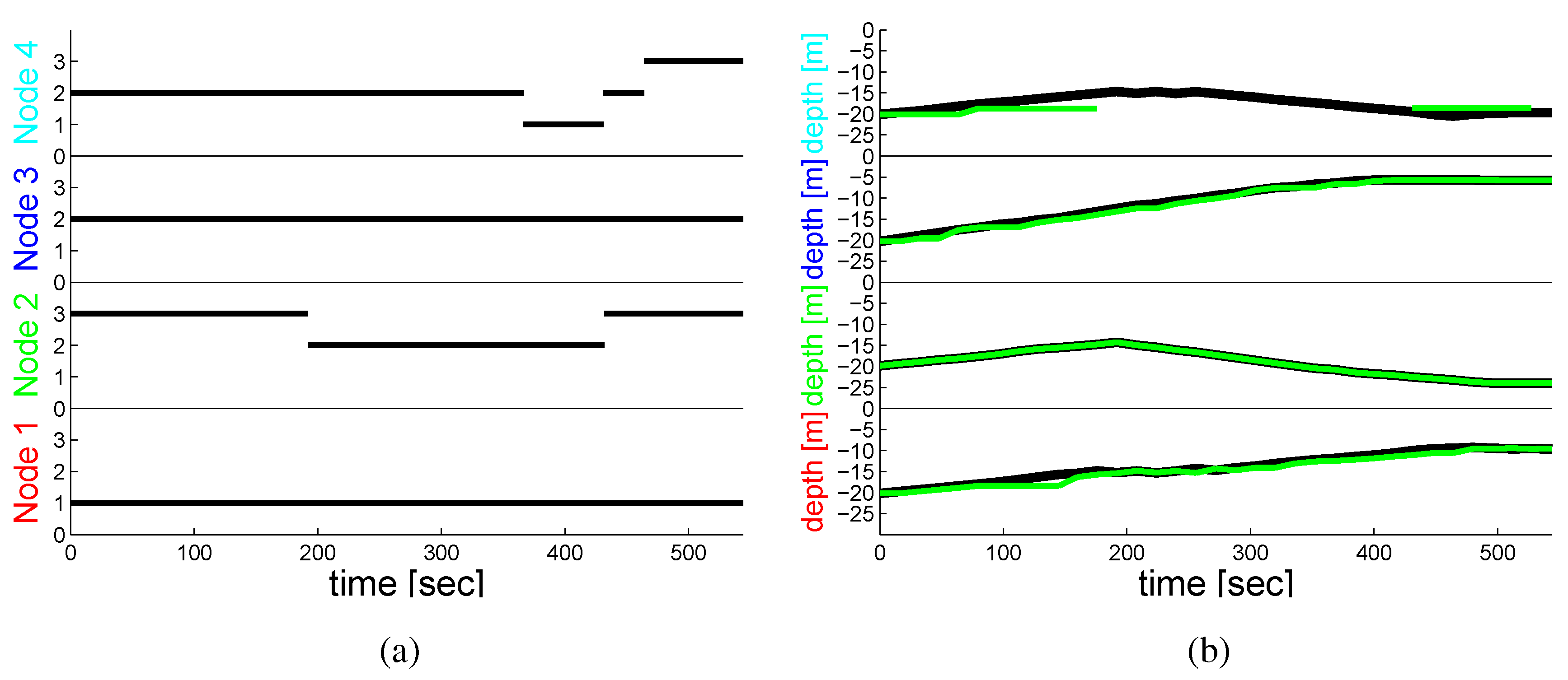
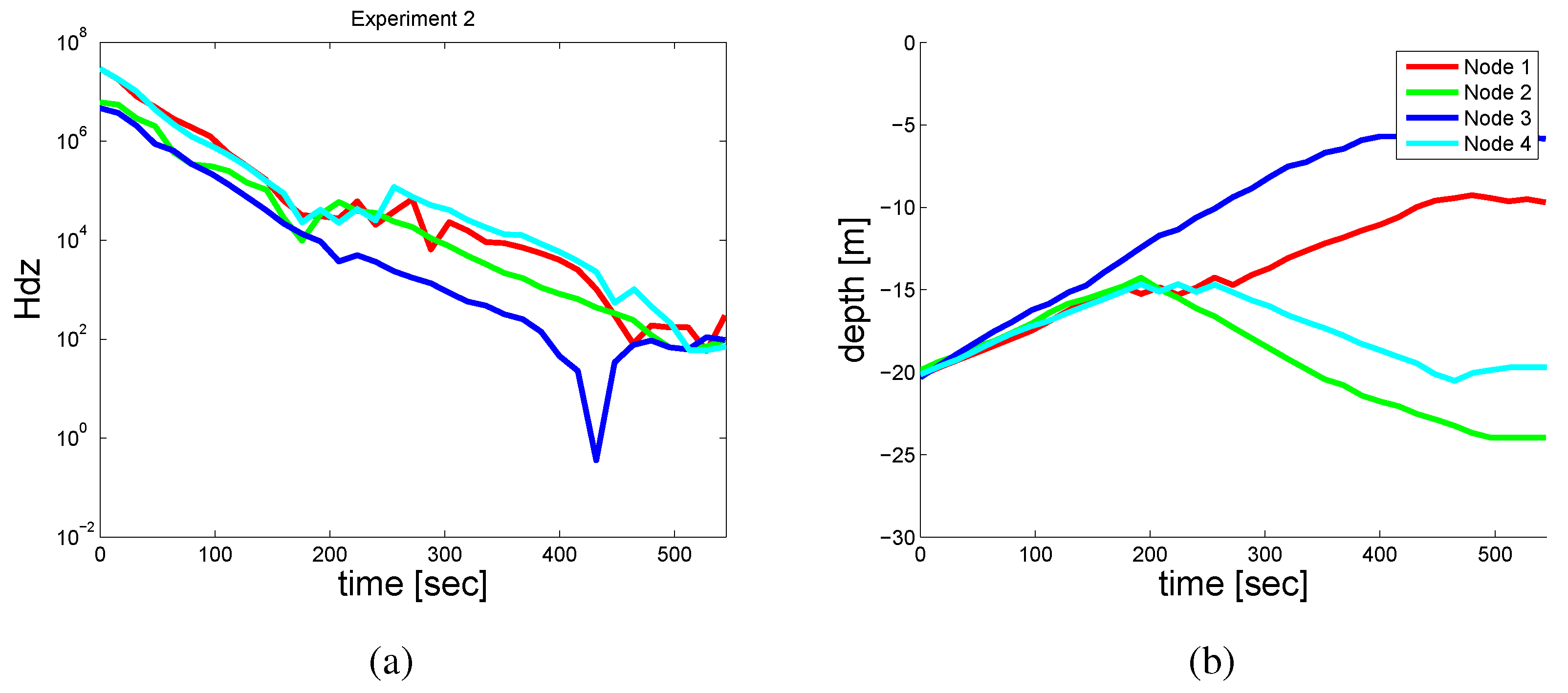
Figure 17.
(a) The value of . (b) The depths over the course of an experiment.
Figure 17.
(a) The value of . (b) The depths over the course of an experiment.
Figure 17a depicts the absolute value of the cost function,
, for each node in the pool while using the Gaussian covariance on a log-scale. Initially, the gradient of the objective function was high; however, over the course of the experiment the value on each node decreased until it reached a stable state. The dip in the objective function for one node seen in
Figure 17a is caused by a temporary configuration that was slightly better from the standpoint of the one node and is magnified by the log-scale of the plot.
Figure 17b shows the depths of each of the nodes over the course of the same experiment. Initially, the nodes were started at 20 m. All of the nodes approached the center of the water column after 200 s. From here Nodes 1 and 3 continued up in the water, while Nodes 2 and 4 returned to a lower depth. The total time to convergence in this experiment was approximately 8 min.
Table 1 shows the start and end configurations for some of the experiments we performed using the Gaussian covariance function. In most of the experiments the controller converged to a configuration where the nodes were oriented in a zigzag configuration. An exception to this is trial Bucket 3 where the nodes initially started in a diagonal configuration. In this case, the nodes converged to a down-up-up-down configuration, a local minimum.
Table 1.
Selected start and end configurations with the base covariance function.
Table 1.
Selected start and end configurations with the base covariance function.
| | Node0 | Node1 | Node2 | Node3 |
|---|
| Bucket 1 Start | 10.0 m | 10.0 m | 10.0 m | 10.0 m |
| Bucket 1 Final | 10.3 m | 24.1 m | 5.9 m | 19.7 m |
| Bucket 2 Start | 20.0 m | 20.0 m | 20.0 m | 20.0 m |
| Bucket 2 End | 19.8 m | 5.9 m | 23.8 m | 10.2 m |
| Bucket 3 Start | 3.7 m | 7.8 m | 12.2 m | 15.9 m |
| Bucket 3 End | 9.5 m | 22.9 m | 23.9 m | 9.6 m |
| Pool 1 Start | 10.2 m | 9.9 m | 10.1 m | 9.8 m |
| Pool 1 End | 20.6 m | 6.9 m | 24.1 m | 10.2 m |
| Pool 2 Start | 20.0 m | 20.1 m | 20.3 m | 20.1 m |
| Pool 2 End | 9.5 m | 23.9 m | 5.6 m | 18.8 m |
| Pool 3 Start | 20.2 m | 19.9 m | 20.3 m | 20.1 m |
| Pool 3 End | 9.6 m | 24.0 m | 5.8 m | 19.7 m |
Table 2.
Selected start and end configurations with river covariance function.
Table 2.
Selected start and end configurations with river covariance function.
| | Node0 | Node1 | Node2 | Node3 |
|---|
| Bucket 1 Start | 1.0 m | 1.0 m | 1.0 m | 1.0 m |
| Bucket 1 Final | 1.6 m | 0.7 m | 0.6 m | 2.4 m |
| Bucket 2 Start | 1.0 m | 1.0 m | 1.1 m | 1.0 m |
| Bucket 2 End | 2.5 m | 1.5 m | 1.7 m | 0.5 m |
| Bucket 3 Start | 1.0 m | 2.0 m | 1.0 m | 2.0 m |
| Bucket 3 End | 0.8 m | 2.4 m | 0.6 m | 2.1 m |
| Pool 1 Start | 1.0 m | 1.0 m | 1.0 m | 1.0 m |
| Pool 1 End | 2.4 m | 1.5 m | 0.5 m | 2.4 m |
| Pool 2 Start | 2.0 m | 2.0 m | 2.0 m | 2.0 m |
| Pool 2 End | 0.7 m | 2.3 m | 0.7 m | 2.2 m |
| Pool 3 Start | 2.0 m | 2.1 m | 2.0 m | 2.0 m |
| Pool 3 End | 0.7 m | 2.8 m | 0.8 m | 2.8 m |
Similarly,
Table 2 shows the start and end configurations for some of the pool and bucket experiments for the river model covariance function. A different local minimum of up-mid-down-up can be seen in trial Pool 2.
Section 6.3.4 explores how different start configurations affect the final positioning of the nodes.
7.1.2. Communication Performance
The acoustic channel is a very low bandwidth, high noise environment. Despite being placed close together in the pool, the communications were similar to what we typically find in river experiments in that all nodes hear single-hop neighbors and some nodes hear farther nodes. This is due to the highly reflective and therefore challenging acoustic environment in the pool [
27,
28,
29].
In our implementation, each node only used depth information from neighboring nodes whose last depth message was received within the past two minutes.
Figure 18a shows the number of neighbors each node used in the calculation of the decentralized depth controller,
. The nodes were in a line in numerical order. Node 1 typically only heard Node 2; Node 2 heard 1, 3, and 50% of the time heard 4; Node 3 heard 2, 4; and Node 4 heard 3 and 20% of the time heard 2.
Figure 18b shows the lag in Node 2’s estimate of the depths of the other three nodes. As we use a TDMA communication algorithm (with a 4 s window), we expect to receive an update from each of the 4 nodes every 16 s. However, due to packet loss the updates may arrive less frequently. Thus, the algorithm may use somewhat old data to calculate the controller output, although never older than 2 min. The experiments in this section show that despite the sometimes poor communication, the decentralized controller converges and is robust.
Figure 18.
(a) Number of neighbors used to calculate . (b) One node’s estimate of the others’ depths versus actual.
Figure 18.
(a) Number of neighbors used to calculate . (b) One node’s estimate of the others’ depths versus actual.
7.2. Charles River Hardware With Changing Covariance
We performed experiments to characterize the performance of the decentralized depth adjustment algorithm when the covariance function changes periodically.
Figure 4 (bottom) shows the concentration of CDOM along the Neponset River based on the model described in
Section 6.2 for 2.0 m and 3.0 m of water. Changes in water level are due to tidal effects.
Figure 4 (top) shows the numeric covariance for each of these plots normalized to fall between zero and one.
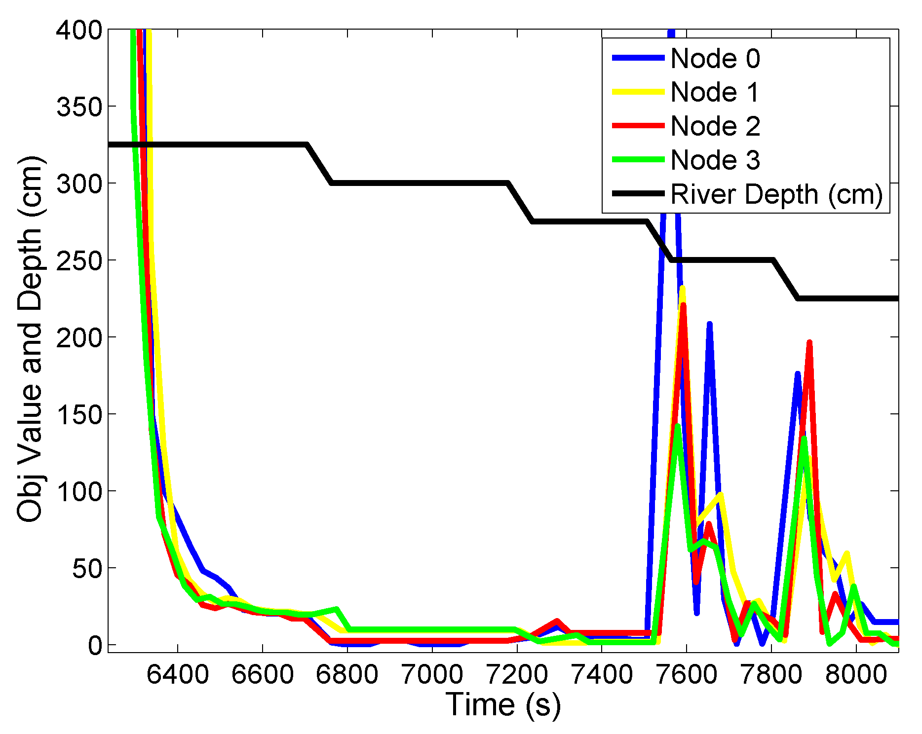
We deployed 4 nodes in the Charles River in Cambridge, MA and simulated updating the covariance function to determine the effect of periodic covariance function updates. We used five different covariance functions based on 3.25 m, 3.0 m, 2.75 m, 2.5 m, and 2.25 m of average water depth.
Figure 19 shows the results. This figure plots the value of the objective function that each node computes over time as well as which covariance function is currently in use (step function at top of Figure).
Figure 19.
Objective value for 4 nodes when changing the depth-based covariance function.
Figure 19.
Objective value for 4 nodes when changing the depth-based covariance function.
In this experiment, the nodes initially had very high objective functions. They then moved, which lowered the objective function. After the nodes stabilized we changed the covariance function from the 3.25 m data to the 3.0 m data. Interestingly, the objective function did not change significantly. Similarly, the transition from 3.0 m to 2.75 m objective function did not have much impact. When moving to 2.5 m, however, the objective function increased greatly. This caused the decentralized controller to adjust the depths of the nodes to again reduce the objective value. A final change in the covariance function from 2.5 m to 2.25 m also resulted in a spike in the objective function, which the decentralized depth controller quickly minimized by changing the depths of the nodes.
This experiment provides initial verification of the hardware system in a river environment. In addition, it verifies that the decentralized controller handles changes to the covariance function in a river environment. Interestingly, some changes to the covariance function result in very minor changes to the value of the objective function, but others cause significant changes.
7.3. Neponset River Experiment
In addition to performing experiments to verify the algorithm in controlled pool and river experiments, we also performed a scientific data collection experiment in the Neponset River, which is located just south of Boston, MA.
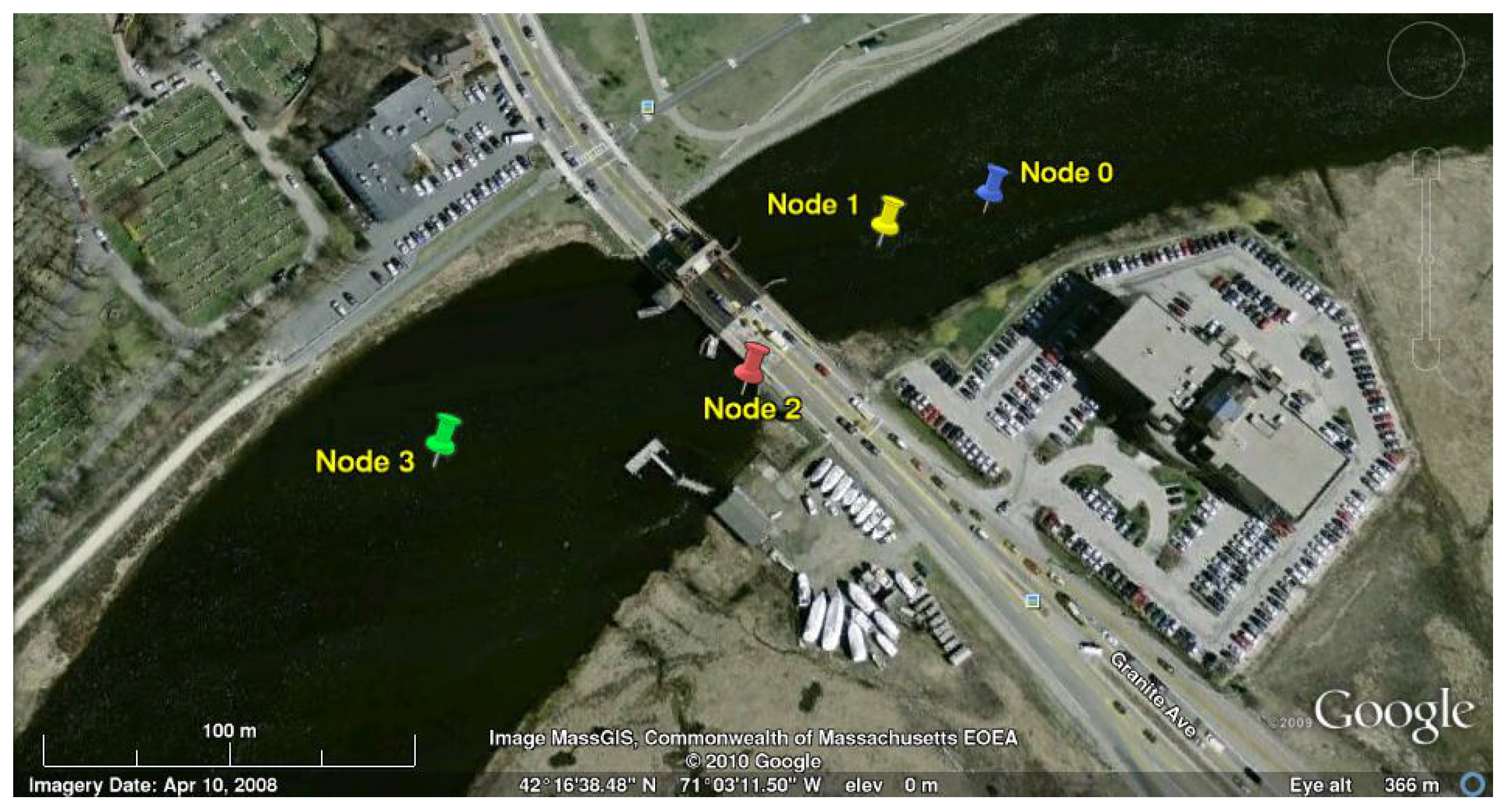
Figure 20 shows a map of the deployment. We deployed four nodes around the Granite Avenue bridge, two on each side of the bridge.
Each node was connected directly to an anchor at the bottom of the river. A length of chain was also attached to the anchor. A rope went from the chain to a surface marker buoy to ensure boat traffic was aware of the sub-surface nodes. The chain allowed us to offset the marker from the location of the anchor and sensor node, reducing the chance of the two lines entangling. We also added an external CDOM sensor to the nodes to collect data. We do not report on this data in detail here, due to lack of space, but we did notice large differences in the CDOM readings at the surface and bottom as predicted by the model.
Figure 20.
Picture of the Neponset River deployment.
Figure 20.
Picture of the Neponset River deployment.
We started the experiment at high tide during which the depth at the deployment locations ranged from 3 m to 6 m. After 7 h we recovered the nodes at low tide. The tidal change was nearly 3 m. After 4.25 h there was a large rain storm that caused significant runoff into the river.
The nodes were programmed to perform column profiles of the water, going to the surface for 5 min and then returning to the bottom for 10 min. In addition, the nodes communicated (using the same TDMA algorithm with 4 s windows per node) and ran the dynamic depth adjustment algorithm. However, we did not control the depths of the nodes using the algorithm, as we wanted a baseline set of data to use to obtain covariance information.
Table 3 summarizes the average time between hearing a messages. The distance from Node 0 to 1 was 35 m, 1 to 2 was 64 m, and 2 to 3 was 93 m. This shows that the nodes were able to hear their single hop neighbors and occasionally a two hop neighbor. It is also apparent from this data that the communication is asymmetric. Node 0 could hear Node 2 much better than Node 2 could hear Node 0. We also observed that the communication had a temporal component (perhaps from tidal changes or current flow as recently observed by Chitre
et al. [
30]). For instance, Node 0 could communicate much better with Node 2 during 2–4 h of the experiment. While the time between communication is fairly high, we note that this is fairly good acoustic communication given the shallow river environment with boat traffic.
Table 3.
Average time, in minutes, between communication during the Neponset River experiment.
Table 3.
Average time, in minutes, between communication during the Neponset River experiment.
| | Node0 | Node1 | Node2 | Node3 |
|---|
| Node 0 | - | 8.3 | 8.1 | 200.7 |
| Node 1 | 4.6 | - | 6.6 | 238.7 |
| Node 2 | 39.0 | 59.0 | - | 46.1 |
| Node 3 | 248.6 | 248.6 | 51.2 | - |
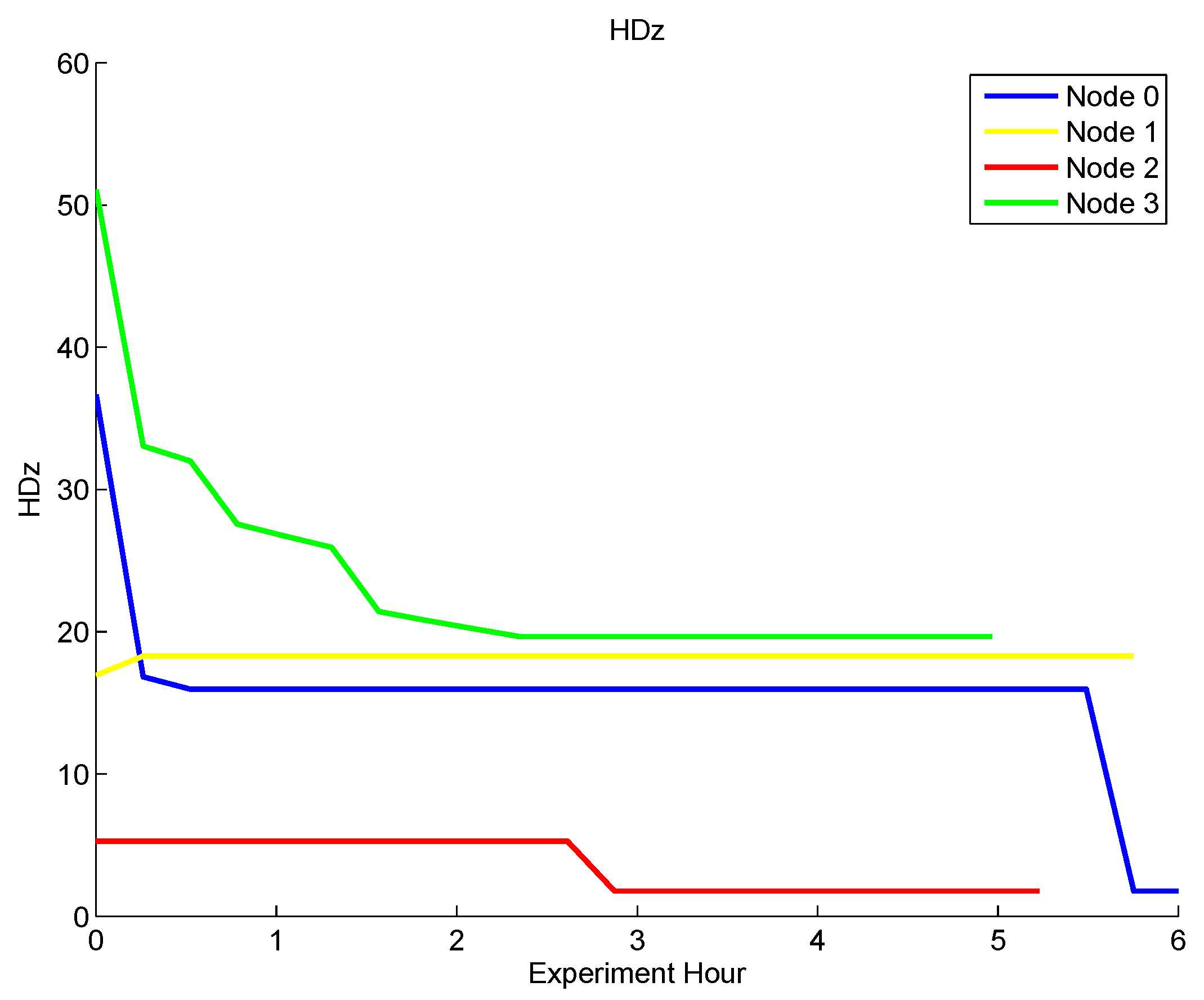
Figure 21 shows the value of the decentralized depth adjustment controller output over the course of the deployment. During the experiment, the gain on the controller output was set low so that it converged slowly. In addition, a deadband of 20 was placed on the controller, meaning that the nodes would not move if the value of HDz was less than 20. This explains why the controller output does not go to zero. In this experiment, we demonstrated the performance of the depth adjustment system and the decentralized gradient controller in a real setting. This verified that the decentralized gradient controller functions in a real river deployment.
Figure 21.
The controller output HDz during the Neponset River experiment.
Figure 21.
The controller output HDz during the Neponset River experiment.
8. Related Work
The algorithm developed in this paper is closely related to previous work in sensor placement and robot path planning to optimize sensing. Here we summarize a few of the many related papers in this area. Cayirci
et al. simulate distributing underwater sensors to maximize coverage of a region by breaking the region into cubes and filling each cube [
31]. Akkaya
et al. simulate optimizing sensor positioning by spreading out the nodes while maintaining communication links in an underwater sensor network with depth adjusting capabilities [
32]. Zhao
et al. present a method for the autonomous navigation of mobile robots using artificial potential field. Their work is different from previous work on potential fields as the controller can keep the robot away from obstacles, escape from local minima, and at the same time prevent the robot from falling into complicated environments where it can get trapped in a local minima [
33]. Our approach is different from these in that we account for sensing covariances, use realistic communication assumptions, and implement and test the algorithm on a real underwater sensor network.
Ko
et al. develop an algorithm for sampling at informative locations based on minimizing the entropy [
34]. Guestrin
et al. introduce the optimization criterion called mutual information [
26]. Mutual information finds sensor placements that provide the most information about unsensed locations. They prove that the problem of picking optimal sensor location is NP-complete and provide a constant factor approximation algorithm. Choi
et al. provide a framework for quantifying the information obtained by a continuous measurement path to reduce the uncertainty in long-term forecast. They represent the environment of the mobile robot as a linear time-varying system and use mutual information between the continuous measurement path and the future verification variables as a means to measure information gain [
35,
36]. Julian
et al. present an approach based on mutual information gradient to control robots equipped with sensors to improve the quality of sensing [
37]. They present a framework for using many collaborating robots equipped with sensors to acquire information from a large-scale environment. The authors assume a non-parametric distribution of data and achieve decentralized control by using a consensus-based algorithm [
38]. They develop a fully decentralized system and carry out indoor and outdoor experiments using five quadrotor flying robots, and then use the developed inference and coordination software to simulate a system of 100 robots [
39].
Leonard
et al. develop controllers to create optimal ellipsoidal trajectories for mobile underwater sensors based on minimizing the posterior error assuming a Gaussian process [
40]. Yilmas
et al. plan a path for an AUV that will decrease measurement uncertainty using a linear programming approach [
41]. Smith
et al. develop a trajectory planning algorithm for underwater gliders to persistently monitor parts of the ocean with minimized deviation from a planned path while balancing the information gain [
42]. This is similar to our approach of balancing sensing versus path length for our robot in our hybrid sensor network-robot setup. Rigby develops an algorithm that uses Monte-Carlo simulations to pick a path for an AUV that minimizes the trace of the posterior covariance matrix assuming a Gaussian process [
43].
Our algorithm differs from these works on sensor placement and path planning in a number of ways. Our algorithm is decentralized and runs in real-time on our underwater sensor network, whereas much of the related work computes placements and trajectories before the deployment. One of the key components of our algorithm that allows us to run in real-time is a choice of an objective function that is easier to compute on a sensor network platform with limited memory and processing capabilities. Most current approaches are based on the minimization of entropy, posterior error, or the use of mutual information. All of these formulations require the computation of the inverse or determinate of the full covariance matrix for the system. These computations exceed the memory and processing capabilities of most sensor network systems. Our system only relies on having the covariance and thus we are able to implement it on our sensor network platform. We show in
Section 6.5 that our algorithm also tends to minimize the posterior error criteria, while requiring less computational complexity. Our algorithm also runs continuously and can adapt to changing conditions.
Further, our algorithm uses a decentralized gradient-descent controller. Cortes
et al. use a decentralized gradient controller to perform Voronoi tessellations for a known event distribution [
44]. Details on these types of algorithms can be found in the book by Bullo
et al. [
22]. Schwager
et al. extend these controllers to learn the underlying sensing function through consensus [
45]. Our work draws inspiration from these techniques but differs in problem specification: our underwater sensors are only able to adjust their depth and are extremely constrained by communication.
Obtaining a covariance function for an underwater system is a problem that has been previously studied and is a common technique. Leonard
et al. use a multivariate Gaussian function, similar to ours, to estimate the covariance in their system [
40]. Lynch
et al. note the historic use of multivariate Gaussian functions to model underwater systems and use stochastically-forced differential equations to analytically determine better covariance models for ocean environments [
2]. They use the covariance models they develop as input into objective analysis models. Objective analysis is statistical estimation under Gauss-Markov conditions. In our system we use a multivariate Gaussian function as a first estimate of the covariance for systems where detailed information is unavailable. For systems with sensed or modeled data, we numerically compute a covariance function based on the actual data. These functions can be updated online as the system runs, which improves their accuracy.
A number of trial and longer-term underwater sensor network systems have been deployed. MOON aims to create an ocean observatory in the Mediterranean Sea for monitoring and forecasting weather, environmental monitoring, and marine research [
46]. MOON is part of the Global Ocean Observing System (GOOS), which was created in the 1980s to monitor all of the world’s oceans [
47]. The Ocean Observatories Initiative (OOI) combines deep-sea buoys, cabled underwater networks, as well as independent AUVs and sensors [
48,
49]. Jannasch
et al. have developed a system of statically moored ocean sensors to monitor environmental processes off the coast of California in Monterey Bay [
50]. Pu
et al. examine the challenges in developing MAC protocols for underwater communication and discuss how to overcome them [
51]. Hollinger
et al. look at planning paths to maximize data collection from underwater sensor networks [
52]. For a good overview of how robot systems have been used for environmental monitoring, see the survey paper by Dunbabin and Marques [
53].
Our depth adjustment system is a novel contribution to the field of underwater sensor networks. Other underwater systems have made use of column profilers; however, they have not been integrated as a key component of the underwater sensor network.
9. Conclusions and Future Work
In this paper we present a gradient-based decentralized controller that dynamically adjusts the depth of a network of underwater sensors to optimize sensing. We prove that the controller converges and extend the algorithm to compute the best path for an underwater robot moving through the network to improve sensing. We implement two covariance models: a multivariate Gaussian model and a model from physics-based hydrodynamics. We perform extensive simulations and experiments on our sensor network platform to verify the functionality.
Deploying underwater sensor networks entails numerous challenges that are not found in most terrestrial sensor networks. First and foremost, the housings must be designed to keep the electronics dry, while maintaining easy access for adding sensors, debugging, and reconfiguring. Finding suitable test locations is also challenging. Acoustic communication, already slow, has even worse performance in confined pools. Rivers and near-shore ocean deployments are difficult due to heavy boat traffic, which makes accessing the sensors challenging and potentially dangerous. In addition, it is nearly impossible to recharge the batteries once deployed. Finally, the enormous size of the ocean makes full sensor coverage unlikely. All of these challenges call for the development of new algorithms and systems that optimize sensing, communication, and energy usage simultaneously.
The depth adjustment system adds a number of capabilities to our underwater sensor network that ease some of these challenges. These include the ability to: surface to use the radio; surface to obtain a GPS location fix; surface to ease node retrieval; surface to recharge via solar panels; go to the bottom to avoid boat traffic; and change depth to optimize other parameters such as communication.
We have performed deployments in the Charles River and preliminary larger scale deployments in the Neponset River with the underwater sensor network nodes with depth adjustment capabilities. In the future we plan to perform long term large scale deployments of the system with the robot acting as a mobile sensor. We are also exploring variations of the algorithm that maintain communication links while optimizing depth for sensing. Finally, we are looking at algorithms to minimize the communication and motion to maximize deployment time.


