The results, in terms of MIMO deconvolution, are presented in this section. The simulation parameters and the metrics are first presented, followed with a description of the experimental setup. The simulated results are analyzed: in this case, the channel is stationary over the duration of the message. Finally, a set of field data is analyzed, where time variations of the channel are observed.
3.1. Experimental Setup
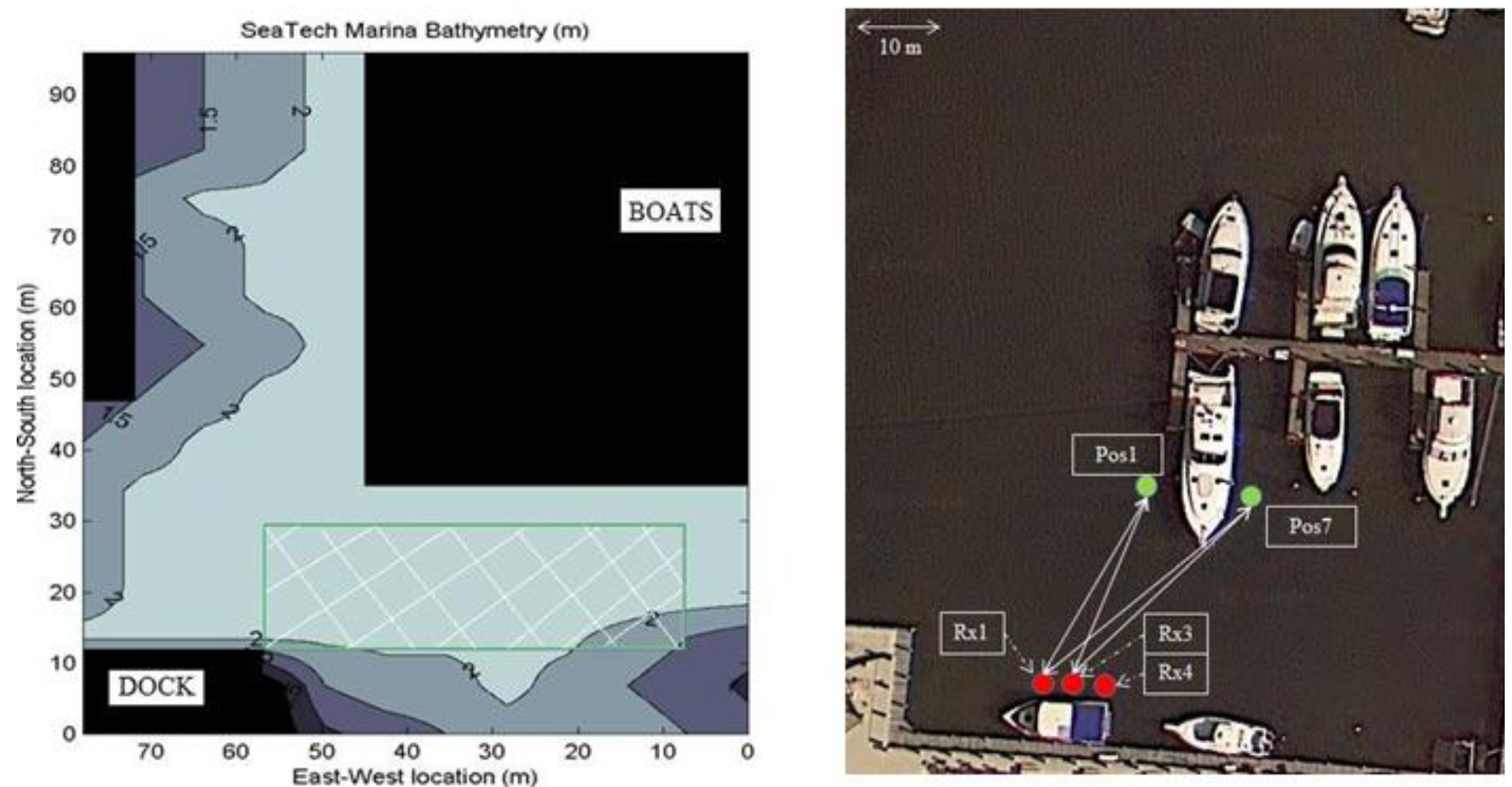
A series of experiments was carried out in the Florida Atlantic University Seatech marina (
Figure 4). While the experimental setup presented here uses two sources and three receivers, this paper presents only the results obtained with two receivers.
Table 1 provides a summary of the data collection. A first set of data was acquired on 27 September 2011. A second series of experiments took place on 31 August 2011. The two sources were alternatively placed at the two locations labeled “Pos1” and “Pos7” in
Figure 4. Two splash proof boxes were built to prevent any damage to the modem sources and were installed on kayaks. Each box contained a set of Hermes source electronics, an ITC-1089 source transducer and a battery pack. The source level was 179 dB ref. 1 μPa at 1 m. The receivers used to carry out these missions were deployed off a small research vessel. The experimental ranges are given in
Table 2. The signals presented in this paper were acquired at a maximum range of 27 m. This short range is mostly due to the high sound absorption loss (100 dB/km at 20 °C and at 300 kHz [
20]).
Since the equipment did not have the ability to perform real-time MIMO communication, each source was used individually and the MIMO messages were constructed off-line. The signal-to-noise ratio SNR
j was calculated at each receiver
j. The value of SNR
j, averaged across every messages within a mission, is shown in
Table 3. The observed SNR value varied between 27.1 dB and 34.3 dB from mission to mission. These variations are mostly due to the time varying characteristics of the channel, which dramatically impacts the average power of the received signals.
Figure 4.
Experimental setup.
Figure 4.
Experimental setup.
Table 1.
Summary of data collected.
Table 1.
Summary of data collected.
| Mission Number and Date | Source 1 Position | Source 2 Position | Receiver 1 Position | Receiver 2 Position | Number of Messages Retained |
|---|
| 1-07/27/2011 | Pos1 | Pos7 | Rx1 | Rx3 | 50 |
| 2-07/27/2011 | Pos7 | Pos1 | Rx1 | Rx3 | 50 |
| 3-08/29/2011 | Pos7 | Pos1 | Rx1 | Rx3 | 100 |
| 4-08/29/2011 | Pos1 | Pos7 | Rx1 | Rx3 | 100 |
Table 2.
Experimental ranges.
Table 2.
Experimental ranges.
| Distance on
Figure 4 | Distance (m) |
|---|
| Rx1-Pos1 | 24 |
| Rx1-Pos7 | 27 |
| Rx3-Pos1 | 23.3 |
| Rx3-Pos7 | 25.8 |
| Pos1-Pos7 | 6.15 |
| Rx1-Rx3 | 2.68 |
Table 3.
Signal-to-noise ratio per mission and per receiver.
Table 3.
Signal-to-noise ratio per mission and per receiver.
| Mission Number and Date | SNR1(dB) | SNR2(dB) |
|---|
| 1-07/27/2011 | 27.1 | 27.3 |
| 2-07/27/2011 | 28.8 | 27.8 |
| 3-08/29/2011 | 30.9 | 34.3 |
| 4-08/29/2011 | 29.2 | 33.2 |
3.2. Simulation Parameters
The channel model, presented in detail in [
4,
17], combines a deterministic model (to determine the average echo intensities) [
15,
16] and a stochastic Rician model (to add some random fluctuation to every echo intensity) [
4]. Sources and receivers’ separation and depth match the experimental setup presented in
Section 3.1.
The simulation parameters (
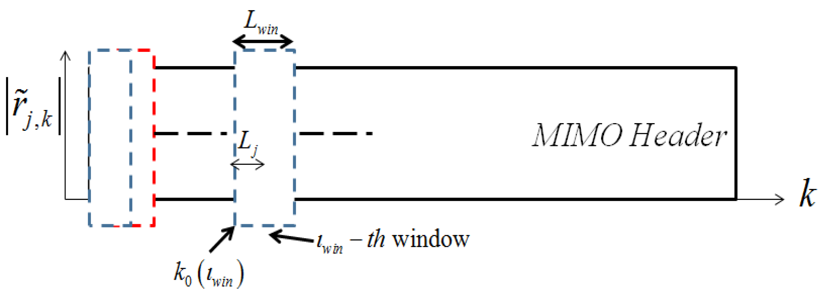
Table 4) are tuned to match the experimental data sets as closely as possible. Doppler shift and Doppler spread have been derived from the field data. The time window used to perform the channel estimation covers the duration of the MIMO sequence and the dead-time interval. Hence, the channel is assumed to be time-invariant over the transmission of a message. The coherence time of the channel therefore corresponds to the total length of the transmitted message: each new transmission would lead to a different channel to estimate.
For every transmitted message, we also adjust the time delay
τ0 between the signals measured at every receiver. In this paper, we only consider full overlap between received messages. The results for partial overlap are presented in [
17]. The channel model considered here includes both the specular reflection from the sea bottom and scattering from the sea surface and bottom.
Table 4.
Simulation parameters. Some of the simulation parameters are not formally used in the equations listed in this paper. The parameter name is followed with references [
4,
17], where the equations using these parameters are provided.
Table 4.
Simulation parameters. Some of the simulation parameters are not formally used in the equations listed in this paper. The parameter name is followed with references [4,17], where the equations using these parameters are provided.
| Name | Symbol | Value (units) | Name | Symbol | Value (units) |
|---|
| Sources Depth [4,17] | DSi | 1 m | Source Level | SL | 179 dB re 1 µPa @ 1 m |
| Receivers Depth [4,17] | DRj | 1.5 m | Noise Level | NL | 83.7 dB re 1 µPa |
| Water Depth [4,17] | DW | 3 m | Sampling Frequency | FS | 150 kHz in base band 750 kHz in pass band |
| Water Sound Speed [4,17] | C | 1,500 m/s | Symbol Rate | Dsym | 75 kHz |
| Water Density [4,17] | ρ | 1,023 kg/m3 | Carrier Frequency | f0 | 0 kHz in base band
300 kHz in pass band |
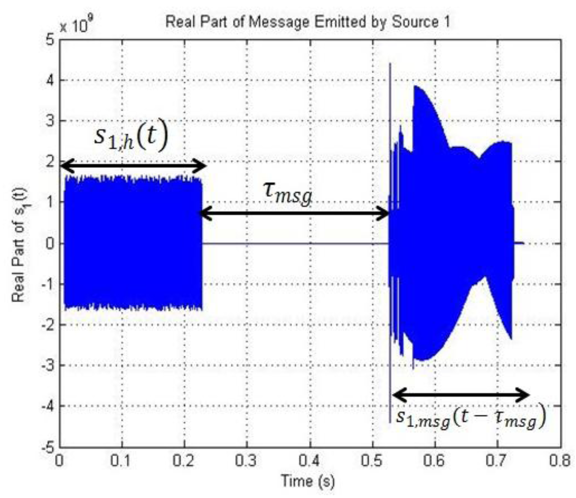
| Sandy Sediment Sound Speed [4,17] | Cb | 1,800 m/s | MIMO Sequence Duration | τh | 218.5 ms |
| Sandy Sediment Density [4,17] | ρb | 1,800 kg/m3 | Dead-Time Duration | τmsg | 300 ms |
| Sea Bottom Loss [4,17] | LSB | 5 dB | Correlation Threshold Parameter | Kthr | 20 |
| Beginning of Time Window [4,17] | k0 | 0 | Time Window Length | τwin | 518.5 ms |
| Number of Transmitters [4,17] | Nt | 2 | Number of Receivers | Nr | 2 |
| Distance Source 1 Receiver 1 [4,17] | R11 | 23.3 m | Distance Source 1 Receiver 2 [4,17] | R12 | 24 m |
| Distance Source 2 Receiver 1 [4,17] | R21 | 25.8 m | Distance Source 2 Receiver 2 [4,17] | R22 | 27 m |
3.4. MIMO Channel Estimation Results
Table 5 shows the values of RMSE
CE as a function of
TL for both experimental and simulated data. The maximum value of
TL is 5.33 ms, as higher values of
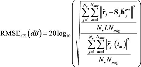
TL lead to singularities and does not produce accurate results. As a reminder, RMSE
CE measures the error between the received signals and the emitted sequences convolved with the estimated channels. RMSE
CE is averaged across every receiver, so that the results presented in
Table 5 translate the accuracy of the channel estimation across every sub-channel.
Table 5.
Relative root mean-squared errors (RMSECE) as a function of TL.
Table 5.
Relative root mean-squared errors (RMSECE) as a function of TL.
| TL(ms) | Simulated RMSECE (dB) | Experimental RMSECE (dB) |
|---|
| 0.667 | −9.5 | −0.4 |
| 1.333 | −12.5 | −0.9 |
| 2.0 | −18.8 | −4.1 |
| 2.667 | −34.7 | −4.9 |
| 3.333 | −34.7 | −6.2 |
| 4.0 | −34.7 | −9.1 |
| 4.667 | −34.8 | −11.4 |
| 5.33 | −34.8 | −25.7 |
In both experimental and simulation cases, as
TL increases, the accuracy of the channel estimation improves. However, while RMSE
CE reaches a sweet-spot at
TL = 2.667 ms using simulated data (
![Jsan 02 00700 i053]()
), the experimental results on RMSE
CE differ. Indeed, the minimum RMSE
CE is obtained for
TL = 5.33 ms (RMSE
CE = −25.7 dB) as shown in
Table 5 and
Figure 5. If, as explained earlier on, values higher than
TL = 5.33 ms cannot be considered, the minimum value of RMSE
CE using experimental data is of the same order of magnitude as RMSE
CE in the simulation framework. The channel estimation can therefore be considered as very accurate.
Figure 5 displays the influence of
TL on the channel estimation accuracy in the specific case of mission 4.
Figure 6 shows that RMSE
CE drops and the confidence interval [−
σCE;
σCE] gets narrower as
TL increases.
Figure 5.
RMSECE and RMSECE ± σCE as a function of TL.
Figure 5.
RMSECE and RMSECE ± σCE as a function of TL.
The SNR is simply computed as the ratio of the received MIMO header power over the ambient noise power. It is also interesting to look at the impact of the SNR on the channel estimation performance for every receiver and every mission carried out. The best possible estimation of the channel impulse response is obtained when RMSE
CE at the output of the channel estimator (Equation (28)) is the inverse of the SNR. In this ideal case, the relationship can be rewritten in dB,
where the SNR is simply computed as the ratio of the received MIMO header power over the ambient noise power.
In the more realistic case of imperfect channel estimation, Equation (4) should account for the residual error in estimating the channel impulse response at receiver
j. This error can be modeled as an additive noise
![Jsan 02 00700 i054]()
, such that:
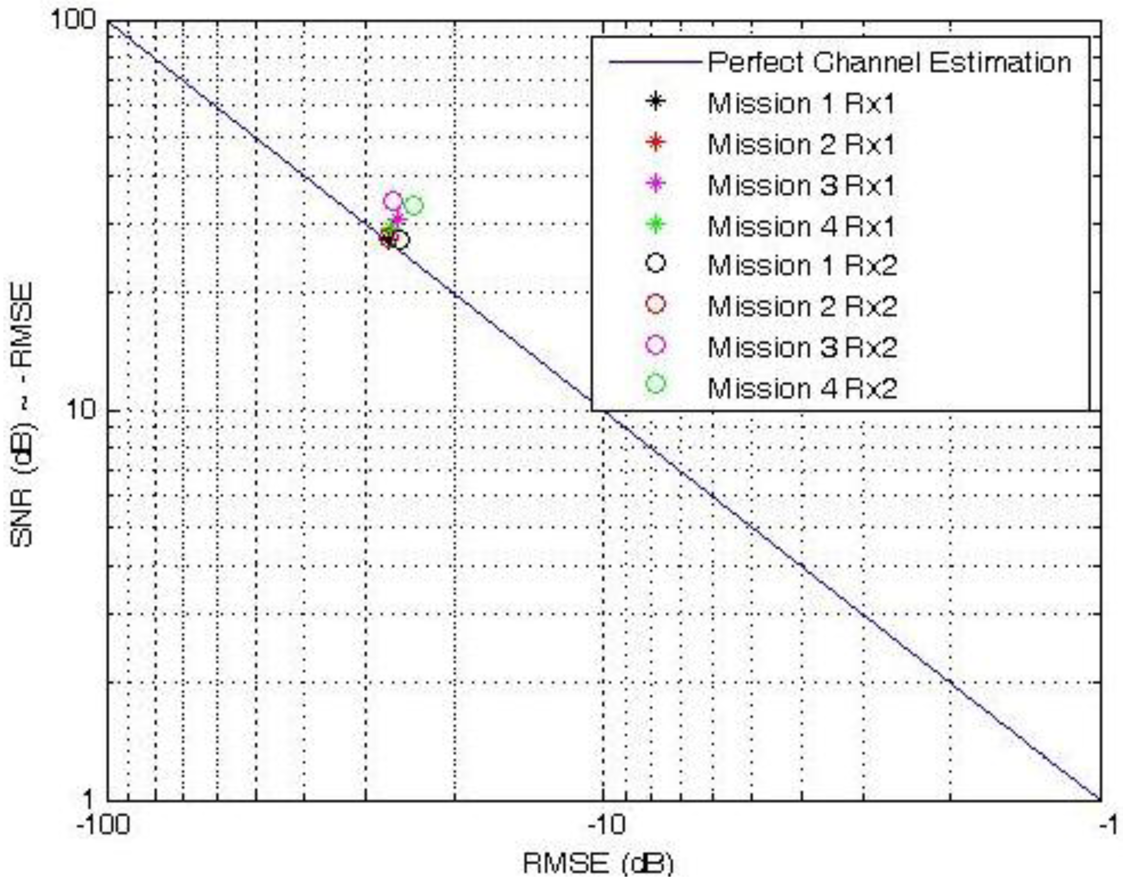
We can verify the validity of such an approximation by comparing the SNR as shown in
Table 2 and the RMSE
CE(dB) (Equation (28)) obtained for each of the corresponding four missions and for each receiver. In theory, when the best possible estimation of the channel impulse response is calculated, Equation (32) applies, as shown using a solid line in
Figure 6. The experimental results, labeled as individual points in
Figure 6, remain very close to this theoretical limit, which indicates that the channel estimation algorithm works very well indeed. For example, the channel estimation in the data set recorded during in mission 2 at receiver 2 results in a value of RMSE
CE (dB) that is almost exactly the opposite of
SNR(
dB). Some discrepancies are also observed, as in mission 3 at receiver 2. In this case, the channel estimator produces significant amounts of additive noise.
Figure 6.
SNR(dB) vs. RMSECE(dB) at the output of the channel estimator.
Figure 6.
SNR(dB) vs. RMSECE(dB) at the output of the channel estimator.
3.5. MIMO Deconvolution Results
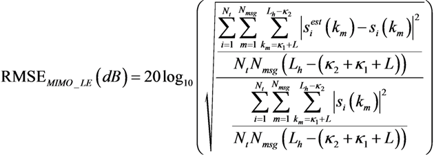
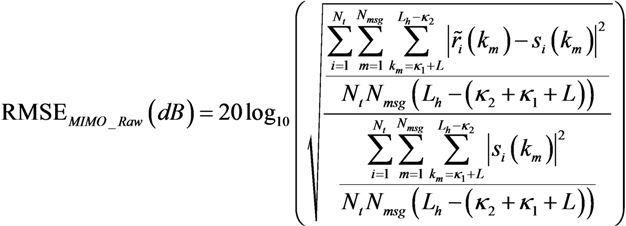
A comparison of the MIMO deconvolution capability between experimental data and simulation results has been completed, using the metrics defined in Equations (29)–(31). The results are shown in
Table 6 and
Table 7. The impact of the parameter
TL on the performance metrics is clearly observed. The results are shown for
![Jsan 02 00700 i056]()
, which lead to the lowest RMSE values [
17]. Both simulations and experimental results (averaged over the total number of missions carried out) are presented in
Table 6. Clearly, RMSE
MIMO_LE and RMSE
MIMO_ICLE decrease as
TL increases using either simulated or field data. Note that the equalizer length is limited to
TL = 5.33 ms, as higher values of
TL led to singularities.
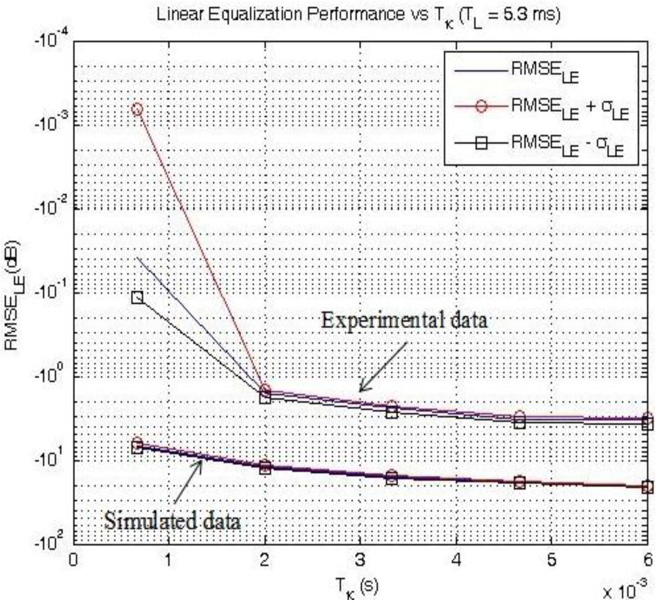
RMSE
MIMO_LE, computed with both simulated and experimental data, is shown in
Figure 7.
Figure 7 shows the influence of the pre-cursor and post-cursor length: if
TL is sufficiently large to provide accurate channel estimation, RMSE
MIMO_LE drops as
Tk increasing. Therefore, showing the influence of
TL on RMSE
MIMO_LE is not of great interest: this is why we chose to represent RMSE
MIMO_LE as a function of
Tk only (
TL = 5.33 ms). For example, for an equalizer length
TL = 5.33 ms, RMSE
MIMO_LE = −6.2 dB with
Tk = 0.7 ms and drops to RMSE
MIMO_LE = −20.5 dB with
Tk = 6.0 ms. As it has been shown in the channel estimation process results, the confidence interval also narrows as the process gets more and more reliable.
Table 6.
RMSE between emitted and (Raw) received signals, RMSEMIMO_Raw as a function of TL.
Table 6.
RMSE between emitted and (Raw) received signals, RMSEMIMO_Raw as a function of TL.
| TL (ms) | RMSE
MIMO_Raw (dB) |
|---|
| Simulations | Experiments |
|---|
| 0.667 ms, 1.333 ms, 2 ms, 2.667 ms, 3.333 ms, 4 ms, 4.667 ms, 5.33 ms | 0.04 | 3 |
Table 7.
RMSE between emitted and received Signals after LE processing, RMSEMIMO_LE and after ICLE processing, RMSEMIMO_ICLE as functions of TL.
Table 7.
RMSE between emitted and received Signals after LE processing, RMSEMIMO_LE and after ICLE processing, RMSEMIMO_ICLE as functions of TL.
| | RMSE
MIMO_Raw (dB) | RMSE
MIMO_ICLE (dB) |
|---|
| Simulations | Experiments | Simulations | Experiments |
|---|
| TL (ms) | 0.667 | 0.4 | 19.7 | −4.5 | 15.8 |
| 1.333 | −3.4 | 14.4 | −6.7 | 12.1 |
| 2.0 | −10.3 | 8.3 | −13 | 6.4 |
| 2.667 | −20.5 | 5.5 | −33.4 | 3.1 |
| 3.333 | −20.5 | 2.2 | −33.4 | 0.7 |
| 4.0 | −20.5 | −1.9 | −33.3 | −3 |
| 4.667 | −20.5 | −3.9 | −33.3 | −8.8 |
| 5.33 | −20.5 | −3.3 | −33.2 | −26.9 |
Figure 7.
RMSEMIMO_LE as a function of TL and Tk using simulated data.
Figure 7.
RMSEMIMO_LE as a function of TL and Tk using simulated data.
In the case of experimental data, severe distortions in the received signals impact the accuracy of the MIMO deconvolution process. Indeed,
Tk = 6.0 ms varies dramatically when computed with simulation and experimental data. In the best case scenario, we use
TL = 5.33 ms and
Tk = 6 ms.
Table 7 shows that RMSE
MIMO_LE = −3.9 dB using real data
vs. RMSE
MIMO_LE = −20.5 dB using simulated data. Nevertheless, the LE process on experimental data dramatically improves the quality of the received signal:
Table 6 shows that RMSE
MIMO_Raw = 3 dB whereas
Table 7 shows that RMSE
MIMO_LE = −3.3 dB when
TL = 5.33 ms.
The relatively significant differences between simulation and field data performances are related to the time-varying characteristics of the experimental channel but also to co-antenna interferences. Indeed, the experimental channel impulse responses presented a coherence time much shorter than in the simulation case, leading to a lack of accuracy in the co-antenna interference removal process.
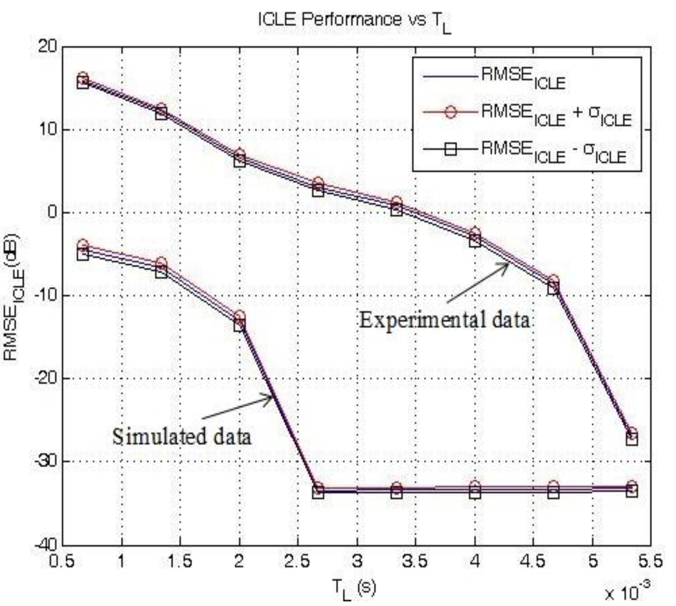
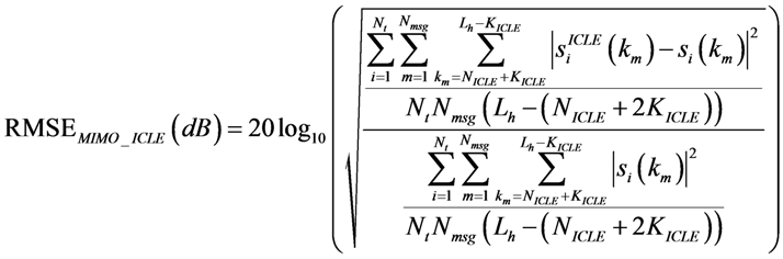
Figure 8 shows the variation of RMSE
MIMO_ICLE as a function of
TL: if the MIMO sequence is known, the accuracy of the process improves as
TL increases. On average, RMSE
MIMO_ICLE = −26.9 dB when
TL = 5.33 ms using experimental data
vs. −33.2 dB using simulated data.
Figure 8.
RMSEMIMO_ICLE and RMSEMIMO_ICLE ± σICLE as a function of TL.
Figure 8.
RMSEMIMO_ICLE and RMSEMIMO_ICLE ± σICLE as a function of TL.
As expected, the comparisons between RMSEMIMO_ICLE and RMSEMIMO_LE calculated using simulated and experimental data reveals that LE process does not reach the lower bound provided by ICLE structure. Using simulation data, we find that RMSEMIMO_ICLE = −33.2 dB while RMSEMIMO_LE = −20.5 dB. This phenomenon is especially pronounced in the case of experimental data, where RMSEMIMO_ICLE = −26.9 dB and RMSEMIMO_LE = −3.3 dB for TL = 5.33 ms. One can conclude that LE alone is not totally sufficient to remove the whole interference terms provided by the frequency selective channel and multi-antenna architecture. Non-linear approaches like iterative processing strategy or decision feedback equalization appear thus necessary.


 at receiver j can be written in matrix form [4,17]:

 represents the augmented source signal array at the j th receiver.
  represents the augmented channel impulse response array.
  represents the noise array.
 . Finally, Tj is the sum of the channel lengths over the total number of transmitters Nt, so that
  .
.

 for every time window index twin,


 and
and  as the received signal and noise over the total number of hydrophones:


 and channel impulse responses
  as:
as:


 ,
,  and
and  are defined as


 ,
,


 is the variance of the noise and
  is the variance of the original sequence SI,K.
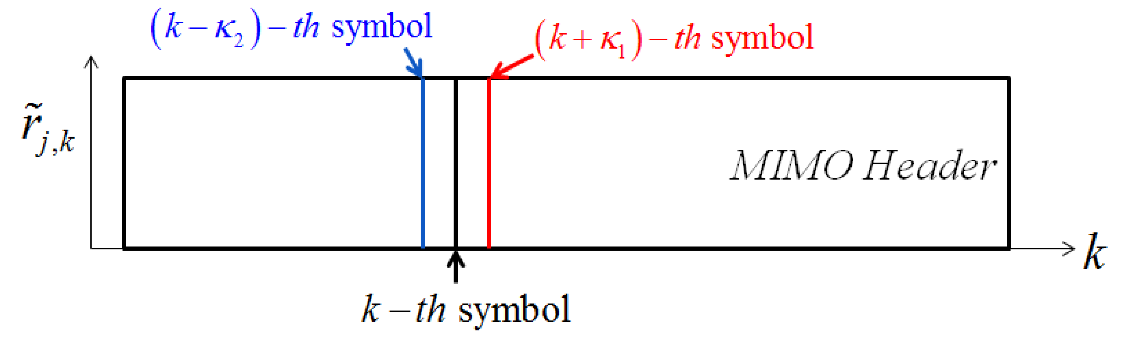
  denotes a column vector of size (L + κ1 + κ2) Nt with 1 at index i and 0 at other positions.
  is the estimates of augmented channel matrix H or time window index twin Here, the estimated signal
  depends on length of the time window, which in turns depends on the measured channel response. If Nwin = 1, the channel is stationary over a message duration and

 becomes a function of twin. In this case, the equalized signal for each sliding window is cropped and forms a section of the equalized output


 depend on the number of time windows used to perform the channel estimation, thus Equations (23)–(25) also apply to

 ), the experimental results on RMSECE differ. Indeed, the minimum RMSECE is obtained for TL = 5.33 ms (RMSECE = −25.7 dB) as shown in Table 5 and Figure 5. If, as explained earlier on, values higher than TL = 5.33 ms cannot be considered, the minimum value of RMSECE using experimental data is of the same order of magnitude as RMSECE in the simulation framework. The channel estimation can therefore be considered as very accurate.
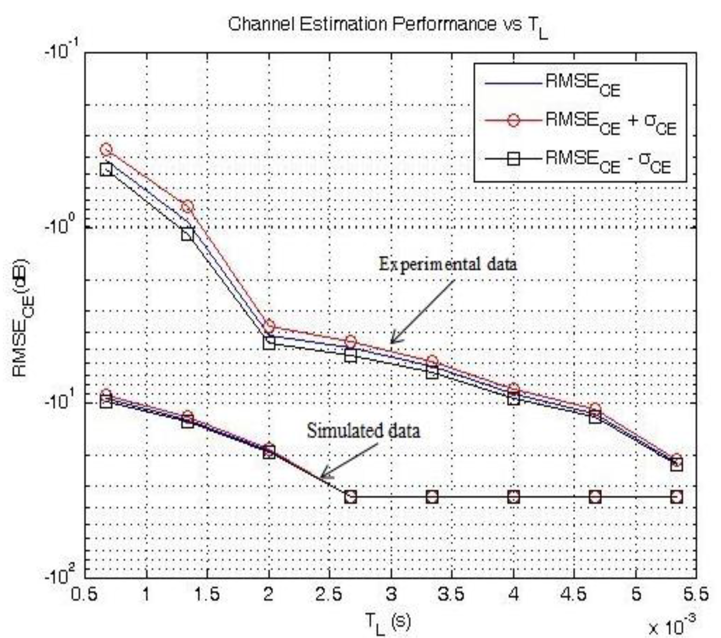
 , such that:

 , which lead to the lowest RMSE values [17]. Both simulations and experimental results (averaged over the total number of missions carried out) are presented in Table 6. Clearly, RMSEMIMO_LE and RMSEMIMO_ICLE decrease as TL increases using either simulated or field data. Note that the equalizer length is limited to TL = 5.33 ms, as higher values of TL led to singularities.
