Road Extraction from VHR Remote-Sensing Imagery via Object Segmentation Constrained by Gabor Features

1
Faculty of Geosciences and Environmental Engineering, Southwest Jiaotong University, Chengdu 611756, China
2
Laboratory for Environment Computation & Sustainability of Liaoning Province, Institute of Applied Ecology, Chinese Academy of Sciences, Shenyang 110016, China
3
Nuclear Industry Huzhou Engineering Investigation Institute, Huzhou 313000, China
4
Department of Land Surveying and Geo-Information, The Hong Kong Polytechnic University, Hong Kong, China
*
Authors to whom correspondence should be addressed.
ISPRS Int. J. Geo-Inf. 2018, 7(9), 362; https://doi.org/10.3390/ijgi7090362
Submission received: 8 August 2018
/
Revised: 26 August 2018
/
Accepted: 31 August 2018
/
Published: 2 September 2018
(This article belongs to the Special Issue Data Mining and Feature Extraction from Satellite Images and Point Cloud Data)
Abstract
:Automatic road extraction from remote-sensing imagery plays an important role in many applications. However, accurate and efficient extraction from very high-resolution (VHR) images remains difficult because of, for example, increased data size and superfluous details, the spatial and spectral diversity of road targets, disturbances (e.g., vehicles, shadows of trees, and buildings), the necessity of finding weak road edges while avoiding noise, and the fast-acquisition requirement of road information for crisis response. To solve these difficulties, a two-stage method combining edge information and region characteristics is presented. In the first stage, convolutions are executed by applying Gabor wavelets in the best scale to detect Gabor features with location and orientation information. The features are then merged into one response map for connection analysis. In the second stage, highly complete, connected Gabor features are used as edge constraints to facilitate stable object segmentation and limit region growing. Finally, segmented objects are evaluated by some fundamental shape features to eliminate nonroad objects. The results indicate the validity and superiority of the proposed method to efficiently extract accurate road targets from VHR remote-sensing images.

1. Introduction
Since roads are a principal part of modern transportation, managing and updating road information in the Geographic Information System database is of great concern [1]. Road information is fundamental geographical information playing an important role in many applications, e.g., serving as reference for the recognition of other objects and travel recommendation [2], road navigation, geometric correction of images, and even assisting confidential transmission of color images [3]. Automatic road extraction is an effective and economic way to obtain road information. However, inaccurate extraction from automatic analysis is common due to the great complexity of very high-resolution (VHR) remote-sensing imagery. Some factors that contribute to the difficulty of high-resolution road extraction are: increased data size and superfluous details with progressively higher resolutions, which means more noise interference and processing time; shelters, such as vehicles and trees on the roadside or shadows of artifacts and buildings, although vehicles’ location can be identified by eavesdrops, it breaks the users’ trajectory privacy [4]; the phenomenon of similar objects possessing varying spectra while different objects possessing the same [5], which can easily cause wrong segmentation results by a region-based method; the necessity of finding weak road edges when the spectral representation of the road surface is similar to the background; and, sometimes, the demand for fast acquisition of road information when facing a crisis [6].
Over the past decades, various road-information extraction algorithms have been proposed and can be classified into three types according to Reference [7]: (1) pixel-based; (2) region-based; and (3) knowledge-based methods. Pixel-based methods detect potential roadside information, such as lines, edges, and ridges, by exploiting pixel-level information. Region-based methods first segment images into regions and then track road regions by classification rules. Knowledge-based methods detect roads by using higher information, e.g., a vison-based system, proposed by Poullis and You [8], uses Gabor filtering and tensor voting for geospatial-feature classification and then graph cuts for segmentation and road feature extraction. Methods applying convolutional neural networks (CNN), such as a road-structure-refined CNN (RSRCNN) approach, are used by combining both the spatial correlation and geometric information of roads in a CNN framework [9]. Buslaev and Seferbekov use the fully convolutional neural network of U-Net to extract road networks [10], while a single patch-based CNN architecture is proposed in Reference [11]. Despite these methods showing superior results, their inadequacy in keeping weak, tenuous edges could diminish the completeness of edge information.
Pixel-based edge detection is a fundamental part for some road-extraction works, and typical methods for line-feature detection [12,13] can present fairly complete edge information. This type of road-extraction analysis [14,15,16,17] is largely accomplished by exploring the spatial characteristics of line features. Lisini et al. [18] proposed a method that applies adaptive filters, the response of which was then used to extract linear features and perform connection work. This method depends on different hard thresholds and data-dependent parameters, thus needing quite a lot of user interaction to optimize the parameters. In Reference [19], a novel aperiodic directional structure measurement (ADSM) was used to construct a mask denoting potential road regions; then, the mask was consolidated with canny edges. The limitation of this method is that considerable errors would occur in road regions with shade or occlusion, since both the geometric and spectral features were affected in different degrees. Only taking edge information into account without considering the spectral characteristics of the road regions can also sometimes make it difficult to distinguish road edges from other objects that possess similar geometrical-line features.
The most popular region-based methods first segment images into regional objects via typical segmentation algorithms such as graph cut [20], energy functional analysis [21], the watershed algorithm [22], or a support vector machine (SVM)-based method [23,24]. For segmented objects, Shi et al. [7,25] and Lei et al. [26] used shape features to judge the segmented regions of road or nonroad objects. Applying object-oriented techniques, Kumar et al. adopted a soft fuzzy classifier built on a set of predefined membership functions to identify road objects [27]. Despite the superiority of this method, especially in complex urban areas, the segmentation method is computationally expensive. In References [28,29], regions’ feature vectors having region codes homogeneous to a region are used for comparison during the retrieval of the images. These methods performed well in some circumstances, but excluded difficulties when there were disturbances such as shadows and shelters, on the road surface; when target objects and the backgrounds possess similar spectral representation; and when illumination of the imagery was extreme darkness or brightness, which could lead to a mixture of the target object with the backgrounds. These difficulties can easily cause confused segmenting results, thus leading to a great loss of extraction accuracy.
To solve this, Alshehhi et al. used Gabor energy and morphological features to enhance the contrast between road and nonroad pixels with a graph-based method for object segmentation [30], which combines the potential advantage of line-feature analysis and object segmentation. Likewise, in Reference [31], a self-adaptive mean-shift algorithm was used first to construct edge information, and, together with spectral features, roads were then extracted using the SVM algorithm by integrating spectral and edge information. Fast extraction of road information is sometimes necessary during emergencies. To obtain road information very quickly, Reference [31] adopted object-based image analysis with segmentation based on mathematical morphology, which demonstrated the high road-extraction efficiency of object-based analysis. Although both approaches showed good performance in the final results, reliable road-extraction results for all situations are still lacking.
Several defects existing in most current road-extraction works are taken into consideration by this study, which include: (1) individual analysis for marginal and regional characteristics of target objects without combining the advantages of each; (2) loss of roadside information caused by shelters, shadows, and the phenomenon of foreign bodies with the same spectrum; (3) inefficient road-object tracking process; and (4) neglecting the spatial and spectral diversity of road objects. We also summarize some road characteristics to be studied in the research, including what is given in Reference [1], as well as some additional characteristics that fit our algorithm: (1) spectral characteristics: road regions have nearly the same spectral representation without excessive shelters or shadows on the surface; (2) spatial characteristics: studied roads are long enough to be recognized with nearly parallel road edges and a moderate degree of crook; and (3) image resolution: submeter level in the range 0.1–0.6 m.
In order to recognize more stable and accurate road objects in remote-sensing imagery from complex scenes, we present a method using Gabor features as edge constraints to facilitate object segmentation and region growing. Gabor features are first detected by applying Gabor wavelets with experimentally determined optimum scale and orientations. Because of shelters, shadows, and the similarity of the targets’ and backgrounds’ spectral representation, Gabor features obtained on the roadside sometimes may be discrete; thus, the edges must go through a connection analysis. In the connection analysis, we first apply a window-based method to extract line features with directional consistency. Then, the extracted line features of interest are extended and linked to supplement the completeness of the edge information and they are used as constraints in the segmentation and region-growing process proposed by this article. Finally, potential road objects from segmentation are evaluated by some fundamental shape features.
2. Methods
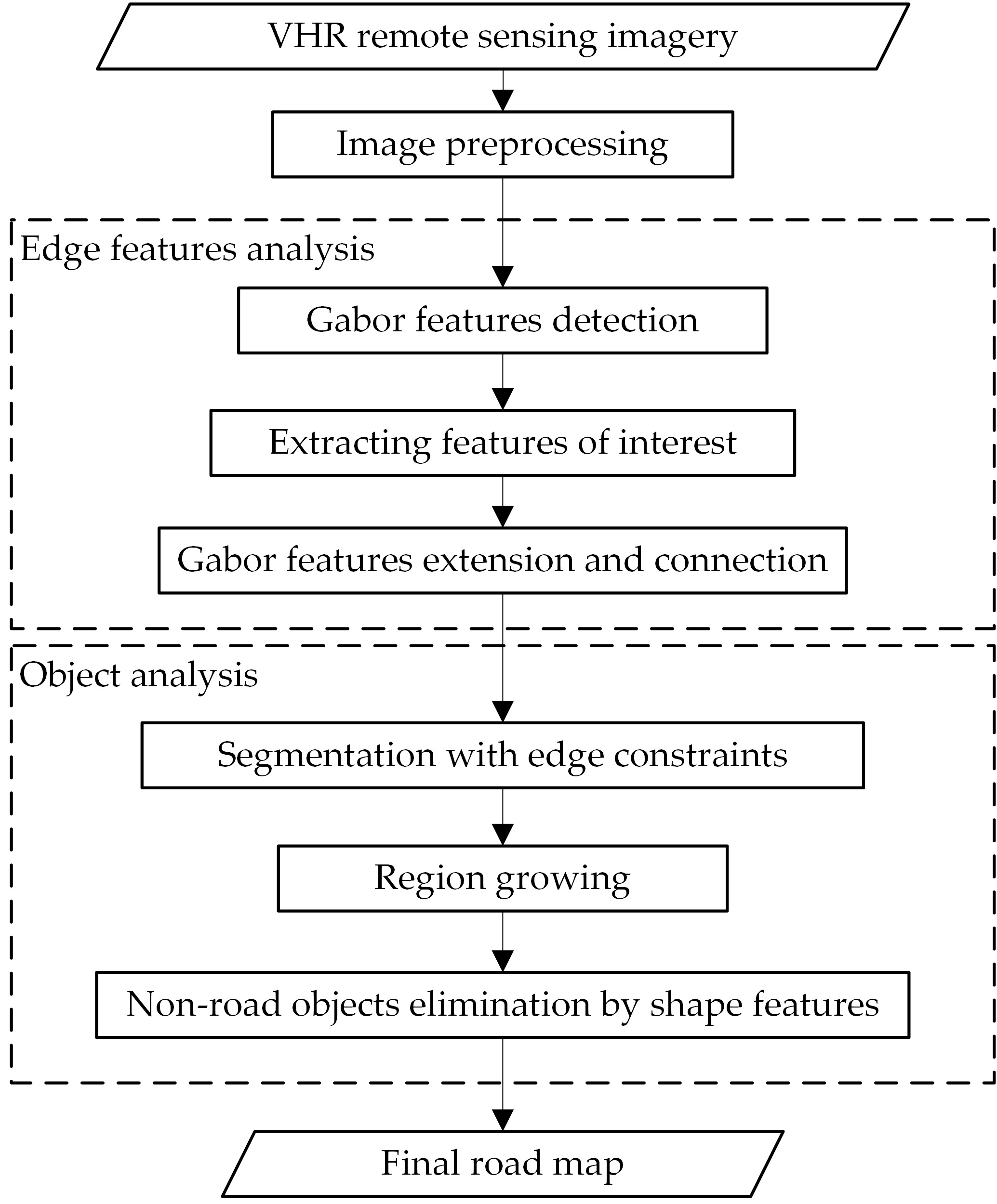
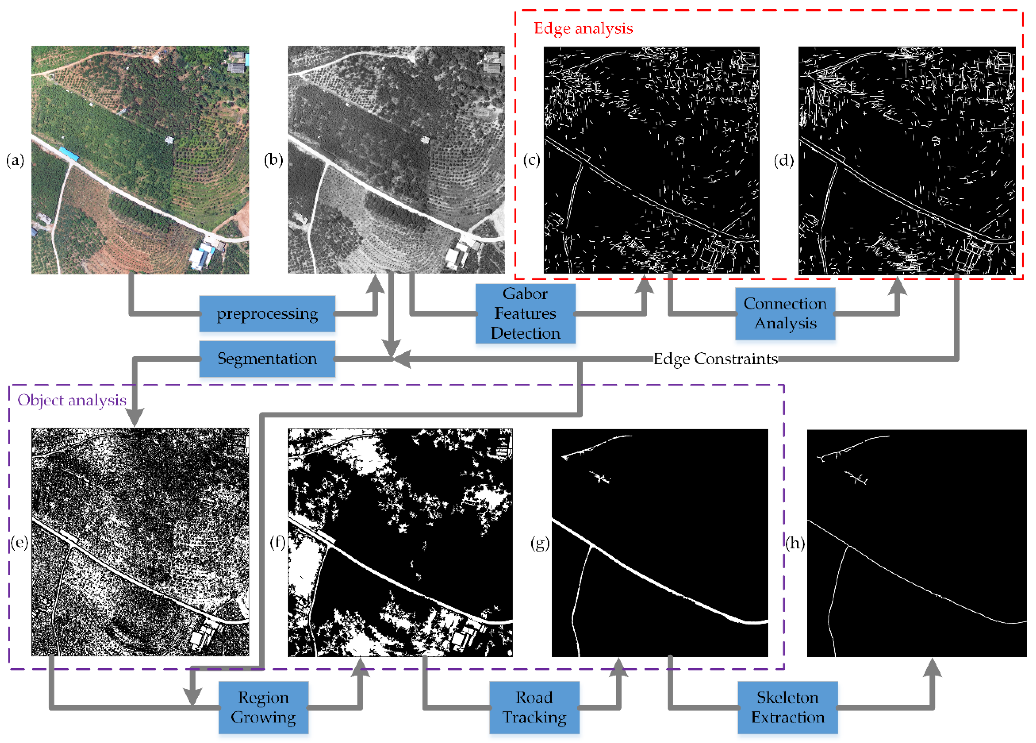
As shown in Figure 1, the two-step automatic road extraction approach is proposed. (1) Edge features analysis: preprocessed imagery was convolved with Gabor wavelet kernels for its invariance to illumination, rotation, scale, and translation, and sensibility to line features to detect responsive features. Then, a window-based method filtered undesired features such as the aforementioned disturbances. After that, to transform the feature analysis in a line-segment-based manner, screened features were processed into line segments by a line-segment detection (LSD) algorithm. Adjacent pair segments were then connected if three criteria were satisfied, which helps supplementing the completeness of line features; (2) object-analysis: connected Gabor features served as edge constraints for segmentation to obtain stable segmented objects. Then, by region-growing, road objects were expanded to complement their missing parts, whereas nonroad objects to highlight nonroad characteristics. Finally, fundamental shape features, including area, shortest inner diameter, complex rate, length–width ratio of the bounding rectangle, and the fullness ratio were used to extract potential target objects.
2.1. Image Preprocessing
The available color image with R, G, and B bands was divided into three grayscale images. Inhomogeneous surface features normally show variant spectral representations in response to different wavelength image sensors. The prominence of the boundary between road and background depends on the spectral variance. Such grayscale images are favored, highlighting the variance. However, it is quite difficult to automatically decide which band is more suitable due to the complexity of the scene. Thus, in this paper, we transformed the color image into a fused grayscale image by using Equation (1):
Random noise distribution in images is inevitable and is always a fundamental aspect of image preprocessing. We adopted bilateral filtering because it not only reduces noise in the image but also protects object edges. After that, we applied a Laplacian operator as a convolution kernel to enhance the image, which provided more favorable inputs for Gabor feature detection.
2.2. Gabor Feature Detection
The original reason that draws our attention to use Gabor filters was the similarity between Gabor filters and the receptive field of simple cells in the visual cortex [32]. With favorable properties that are related to invariance to illumination, rotation, scale, and translation, Gabor filters have been proven successful top performers in many computer-version and image-processing applications, such as biometric authentication (e.g., face detection and recognition, iris recognition, and fingerprint matching) [33]. A Gabor filter is an appropriate linear filter for edge detection and analysis because it provides scale and direction information. There are discrepancies among road-edge-feature responses to filters at different scales. By comparing responses at different scales, target road features more sensitive to the Gabor filter are selected, while recording direction information helps the fundamental analysis of edge-feature connections.
The core of the 2D Gabor filter function for texture-feature extraction can be defined in the spatial domain as follows [34]:
This is a 2D Fourier basis function multiplied by a Gaussian envelope. In the Gaussian part, f is the tuning frequency (wavelength) for scaling, γ is the bandwidth along the major axis, and η is the bandwidth along the axis perpendicular to the major. In the basis function, (x, y) denotes the location and θ the orientation.
The 2D form in Equation (2), created by Daugman et al. [32] from a 1D Gabor core, is only a simplified version. Due to the great magnitude of images, the road-extraction system in this study only takes the real part of the Gabor core into account, since calculation without the imaginary part causes small discrepancies but results in high efficiency in fast target-feature extraction. It is defined in Equation (3):
where is the wavelength, θ is the orientation, φ is the phase offset, σ2 is the variance, and is the spatial aspect ratio.
Gabor bank or Gabor jet, generally taken as Gabor filters, are similar to Gabor wavelets, which derive from the “mother wavelet” (Gabor core) by selecting various combinations of different spatial frequencies and orientations. The mth frequency corresponding to scale information can be defined from [35]:
where k denotes the scaling factor and fmax the maximum frequency. The nth orientations are defined as:
where N is the total number of orientations. To reduce redundant information caused by the nonorthogonality of Gabor wavelets, the approach in Reference [35] selects bandwidth γ by filter spacing k and overlapping p, while bandwidth η by overlap p and N. p = 0.5 has been experimentally proven to have sufficient “shiftability” [33]. Thus, once k, fmax, M, and N are assigned, Gabor wavelets are determined. The multiresolution Gabor feature is shown in matrix form:
Due to the diversity and complexity of remote-sensing images, various object features represent a great amount of discrepancies in different scales [36]. Thus, it is necessary to choose an appropriate scale range that strongly highlights the target objects. The adjustment of scales is an iterative and time-consuming process for each image, let alone for a collection of images. However, for remote-sensing images set where ground features are observed in nearly fixed height and orthographic view, there are only small variances among the best lower and upper center frequencies of interest. In view of that, this study only tested scales in the optimum range (fL, fU), which was adopted for all images. The scales are defined in Equation (4) once fmax = fU is determined and then Gabor features adopting different scales are evaluated.
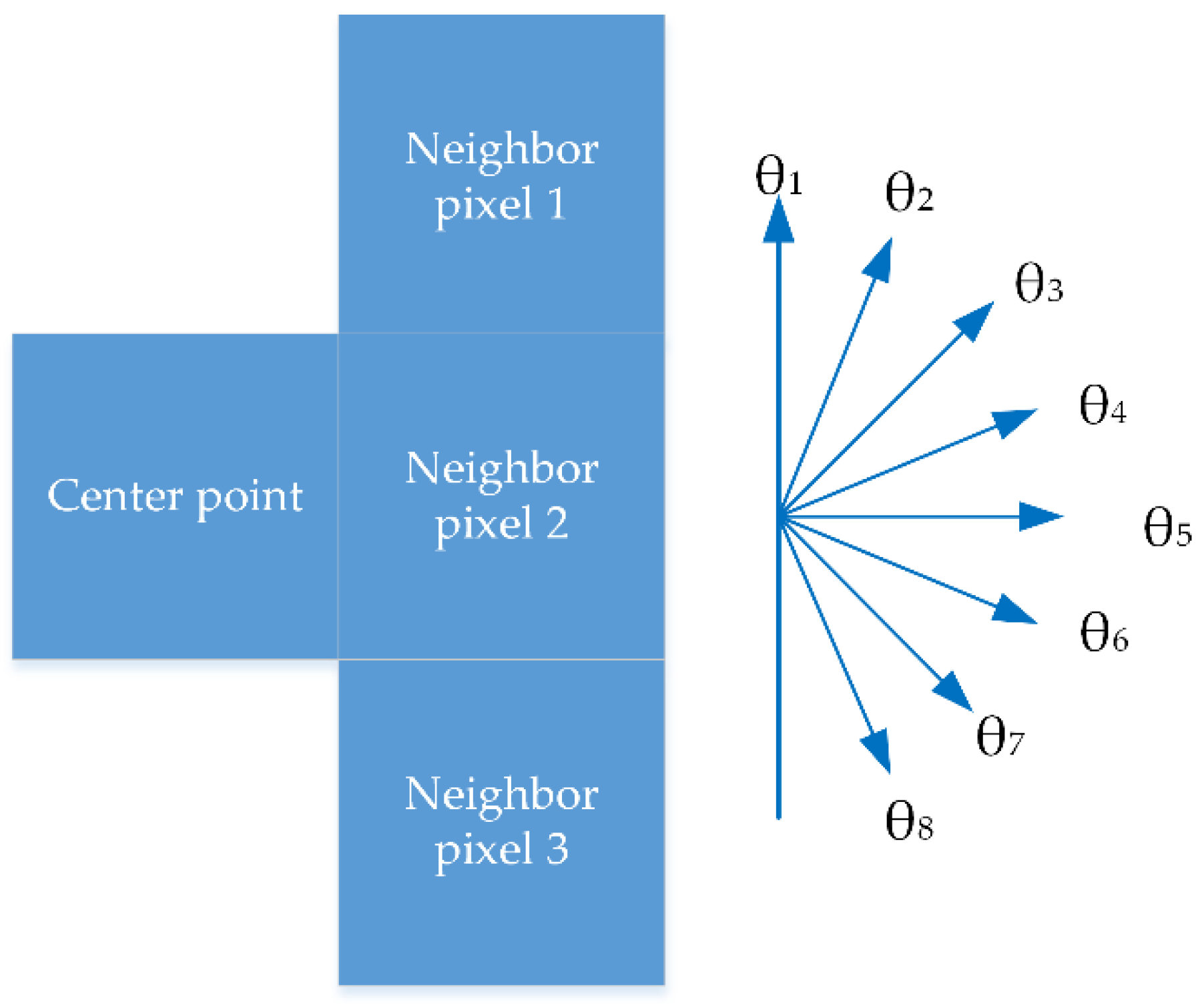
Considering the necessity of recording strong responses and the precise orientation of road recognition and connection analysis, N = 16 was set in this study and proved sufficient for highlighting road features with definite orientation. Gabor features detected in a small range of orientations in some degree represent a strong correlation. It is dispensable to set N as a quite-large value for high direction accuracy while causing great loss in efficiency. When N is too large, convolutions applying these excessive Gabor filters with images would consume unnecessary computational resources. For each scale, there were 16 response maps corresponding to 16 directions. Specifically, if the phase offset φ = 0, we only considered eight directions in the range of [0, π). Figure 2 shows the Gabor bank in eight orientations.
Road features were highlighted in response to Gabor filters by adopting orientations that are similar to road features. Together with many disturbances, they were selected and assigned a corresponding orientation label. The circumstance should be considered when there are disturbances such as vehicles, shadows of buildings and trees, or objects with a nonlinear boundary. Gabor features extracted from these disturbances normally show weak responses and chaotic directions in a small region, while Gabor features from edge noises are generally short line segments with bits of pixels. They can be recognized by setting an area threshold and by judging if the small region has very different multiorientation Gabor features.
To extract responses of interest or to eliminate these disturbances to a certain extent, we proposed a window-based method to evaluate the directional consistency of these features in each response map. The method first defines a window sized a × a, where a is approximately double or triple the road width, and the size is designed to be just enough to contain road edges in the window. By the movement of the window in the images, where the moving lengths were set to half the road width, we extracted features of interest in the window with two rules. The first one was that weak responses below the threshold should be rejected; the other was that a single-feature area should exceed a certain number of pixels, since the features in the same response map satisfied the directional consistency. As shown in Figure 3, disturbed responses to vehicles on road and nonroad objects in Area I and Area II were largely removed by the proposed method while losing only very few road edges.
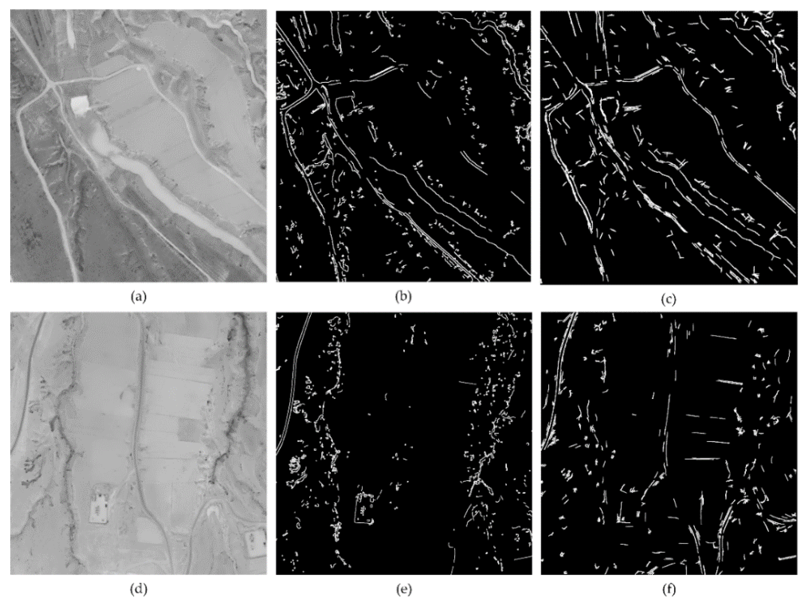
When the extraction work was done, these features of interest were then merged into one map. It is worth mentioning that the method was not merely to extract road edges, but general edge features with potential possibilities to distinguish targets from backgrounds. When facing a scene where edge information is not so conspicuous, it is important to choose an appropriate filter threshold to balance the detection of desired edge features and undesired noises. Figure 4 shows the edge-detection results by the canny algorithm and the proposed method of an origin image in a rural part of Dingbian County, China, with a resolution of 0.4 m, where both the similar spectral representation of dirt roads to the background and the coverage of sand from the background on the road surface make it difficult to maintain the balance mentioned above. From the results, we can see that, for road-edge detection, the proposed method performs better at balancing the detection of “weak edges”, while filtering noises and edges without directional consistency.
Because of the extreme sensitivity to spectral saltation, Gabor features performed well at retaining the completeness of line features to some degree. To make further improvements for completeness, features in the merged response map were first transformed into line segments by LSD analysis [13], which is convenient to use to link adjacent line segments with location and orientation information. This method then lengthened each line segment along its direction pixel by pixel within small distance until the added pixels met “obstacles”, which were pixels in some other line feature or margin of the image. Then, pairwise line segments in the merged map went through a connection analysis considering the following three points: (1) the similarity of two orientations, which is explained by the included angle; (2) if pair segments are close enough to be connected, the distance measure is simply defined as the minimum distance of a point on line 1 to a point on line 2; and (3) if the pair segments are nearly on one straight line, it is determined by calculating the average vertical distance of all points on line 1 to line 2. As shown in Figure 5, θ is the included angle of line 1 and line 3, distance from An to B represents the minimum distance of line 1 and line 2, while the mean value of sum of d1, d2, …, and dn determines whether pair line segments are on one straight line. Figure 6 shows how the connected edge information serves as a constraint for object segmentation.
After the linking process, the merged map was processed with dilation and erosion in a few iterations to merge line segments that were too close to each other. Finally, the processed map was skeletonized. By using Gabor features that were well-suited to detecting weak edges and connecting discrete lines, the problem of mixing target objects and nonroad objects was largely solved. Features with great completeness were then utilized as edge constraints in segmentation and the region-growing process.
2.3. Object Segmentation and Region Growing with Edge Constraints
Much different from pixel-based image segmentation, object segmentation takes into consideration information including spectrum characteristics, texture, shape, and spatial relation. Other then content-based methods exploiting both visual and textual information from multimedia [37,38], this system is mainly concerned with texture and shape characteristics. Initial segmentation is worth considering in order to extract stable road regions without nonroad pixels. Sometimes in a rural area, imaging for road regions and backgrounds appears similar because of the extreme illumination intensity, shadows, and nearly the same spectral characteristics [39]. Especially in road edges bordering upon backgrounds, it is common for road and nonroad pixels to mix, which easily produces false negatives or false positives in subsequent processes for road tracking. Aiming at improving the stability of segmenting road and other objects, a method based on three-band gray consistency in neighboring pixels using Gabor features as edge constraints was used.
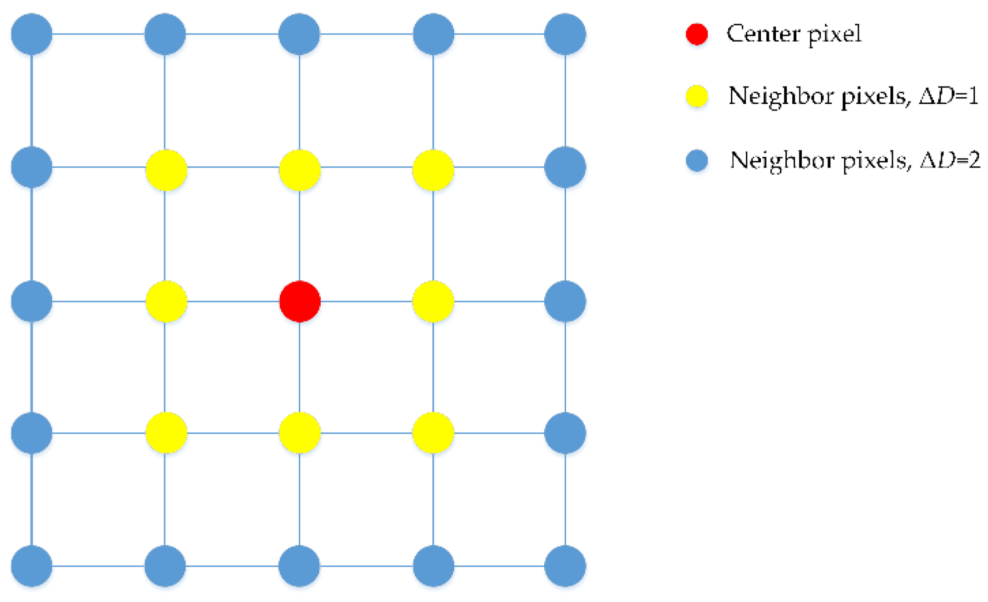
The multichannel imagery combined with the R, G, and B bands was divided into three grayscale images. We first assigned an appropriate neighborhood range ΔD according to the spatial resolution of the imagery set; ΔD determined which neighbor pixels within the range should be taken into account, as shown in Figure 7. For each pixel Pr,i,j(x, y), where r means R band, i means the pixel in the ith row of the image, and j pixel in the jth column, the absolute difference in gray values with its neighbor pixels Pk was assigned to Sr,k, same operations were executed for Pg,i,j(x, y) and Pb,i,j(x, y) to obtain Sg,k and Sb,k. Sk = Sr,k + Sg,k + Sb,k was used to determine whether there was gray consistency between Pk and Pi,j(x, y). Only all neighbor pixels within ΔD satisfied gray consistency; with Pi,j(x, y), we ensured the stability of Pi,j(x, y) belonging to a specific object. Sk, which evaluates pixel stability, was inversely proportional to the possibility of a pixel belonging to certain objects. In the system, a threshold value ST was set to judge the stability of a pixel. If Sk were less than ST, the corresponding pixel was labeled with flag = 1 for its stability. In the other case, the pixel was labeled with flag = 0. Edge constraints were utilized by judging whether Pi,j(x, y) and its neighbors were of pixels on Gabor features. Once the judgement was true, Pi,j(x, y) was ascribed to unstable types and labeled with flag = 0. When all pixels in the image were processed, we assigned gray values of 0 and 1 to Pi,j(x, y) according to its label to obtain the binary image. Details of the segmenting scheme are shown as Algorithm 1:
| Algorithm 1 Objects Segmentation |
| Input: Preprocessed color image and Gabor feature map. Output: Segmented objects map 1 divide color image to R, G, and B grayscale maps 2 foreach Pi, j(x, y) in three maps do 3 if all Pk within range ΔD meet Sk = Sr,k.+ Sg,k + Sb,k < ST then 4 its flagi, j = 1; 5 else 6 flagi, j = 0; 7 end 8 foreach Pi, j(x, y) in Gabor feature map do 9 if gray value of P’i, j(x, y) is greater than 0 then 10 its flagi, j = 0; 11 end |
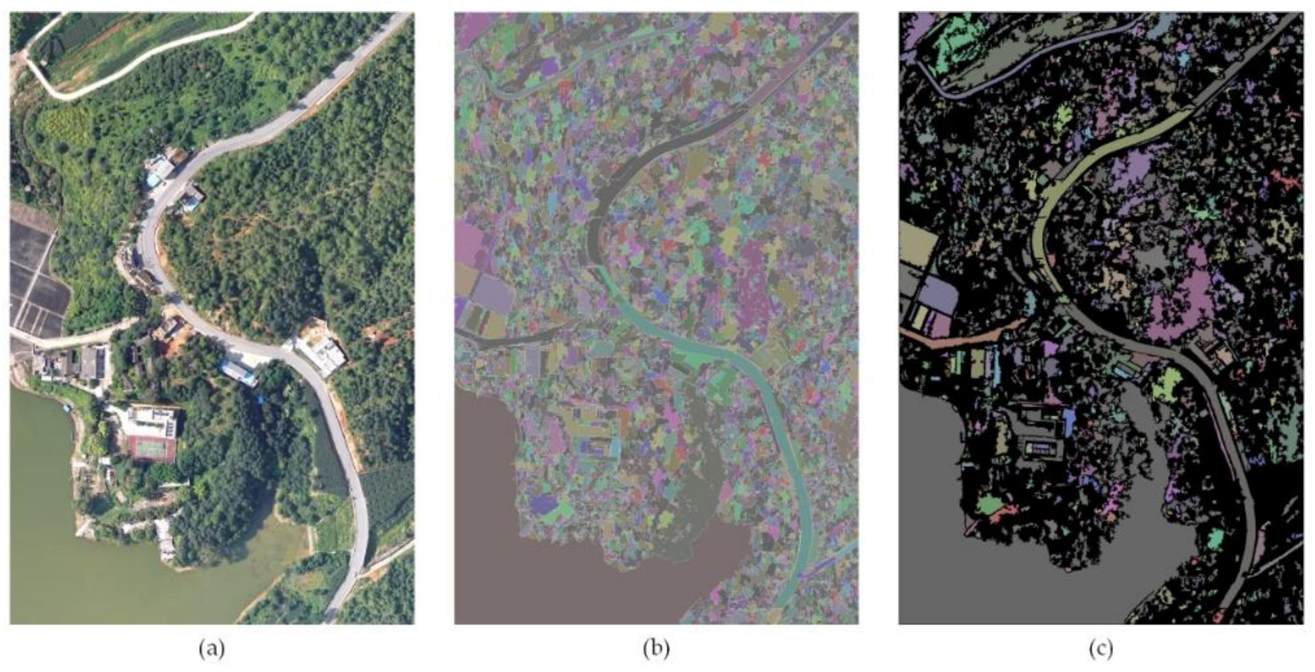
To prove the validity of the proposed segmentation method, we compared the result of this method with the result of the method of Gaetano et al. [22] using the watershed algorithm, and Figure 8 shows the results. As we can see, the proposed method can eliminate unstable pixels on the margins between different objects, which helps to decrease the error classification of uncertain pixels but retains high extraction correctness. The proposed method also shows superior performance in segmentation efficiency and reduces the data size input for road-object tracking.
Sometimes, the method based on three-band gray consistency in neighboring pixels is not enough if there are some nonroad objects such as buildings or an open-pit quarry, which have dissimilar spectral characteristics to road objects. The Gabor filter is sensitive to variations of texture information and can enhance the contrast between road and nonroad pixels [30]. Once there is extreme gray consistency between road objects and backgrounds, it can be solved by using connected Gabor features such as the edge constraints previously mentioned. The detailed operations of applying edge constraints to assist the segmentation process to acquire stable road objects in this system were that, for pixels locating on Gabor features, the gray values were set relatively large so that S would be larger than ST. The results show that all feature pixels and their neighbors were excluded from potential road objects. Despite the guaranteed stability of extracted pixels, the accuracy of road edges decreases. In case of that, a region-growing algorithm was adopted not only to improve accuracy but also to amplify shape-feature discrepancies between road and nonroad objects.
Based on segmented stable objects, a region-growing algorithm with edge constraints was designed to expand road features, and, to some degree, to highlight the nonroad characteristics of other objects. Before the region-growing process, excessively small and large regions obviously not belonging to the road part were eliminated from the area threshold. After that, objects were first labeled by a seed-filling algorithm with different values one to one, for which every pixel in one object was assigned a corresponding value. Then, for each labeled object, an initial pixel on the edge was compared with its four connected pixels successively. Only if the gray values of the initial pixel and its neighbors met certain similarity in the R, G, and B bands, respectively, was the connected pixel incorporated by the object. Once the connected pixel satisfied gray consistency with the initial pixel, it became the next initial pixel to be examined to grow or not. Gabor features played a role as edge constraints in limiting region growing, and pixels locating on them were not allowed to be incorporated. This avoided connection between road objects and backgrounds with gray consistency, since Gabor features went through a connection analysis in which the false connecting problem was largely solved.
2.4. Road-Object Tracking by Shape Features
After the segmentation and region-growing process, segmented objects with stable pixels were evaluated by some fundamental shape features.
2.4.1. Area S
The area (number of pixels) of the road objects cannot be too small or too large. Based on this property, an upper limit threshold Su and a lower limit threshold Sl were set to eliminate nontarget objects. The definition of Su and Sl depends on the spatial resolution of the images. It was common for a few target objects with pixel numbers out of [Sl, Su] to be excluded. However, the loss seemed inevitable because of the great difficulty of these parts to be recognized and correlated.
2.4.2. Shortest Inner Diameter D
The value of the shortest inner diameter D was determined by choosing the shortest diameter calculated from the eight different orientations passing a “center point”. Center points are defined as the points in an object at least three pixels away from the edge. Suppose the center point is a pixel at the edge of the object, as shown in Figure 9. When computing the inner diameter with direction along the direction θ1, the shortest inner diameter could be wrongly assigned 1 pixel width. Since objects segmented in this study were dealt with by the hole-filling algorithm, no hole appeared inside the objects. Obviously, the shortest inner diameter of road region is road width.
2.4.3. Complex Rate C
Complex rate C describes the complexity of a shape and is defined in Equation (7):
where P is the perimeter of the object. For example, C equals 12.6 for a circle, while C equals 16 for a square. The more complex the shape, the larger the value that C equals.
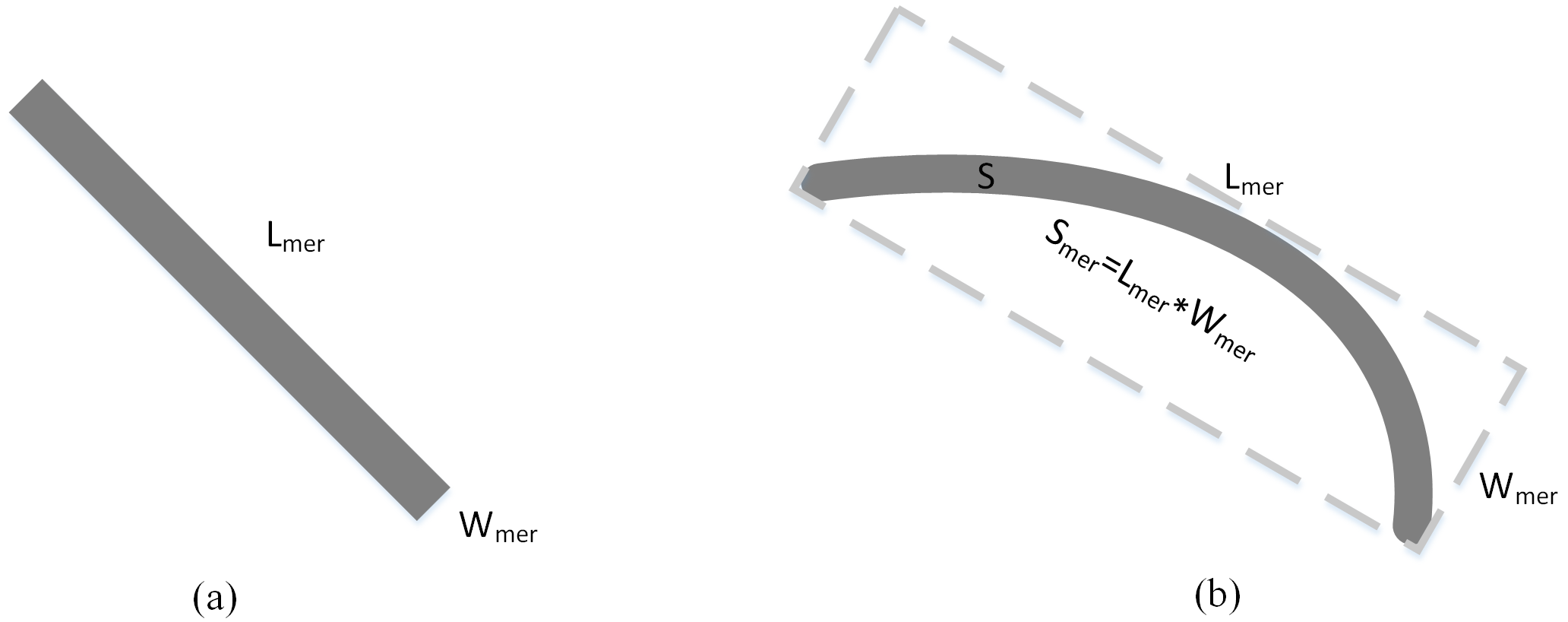
2.4.4. Length–Width Ratio of Bounding Rectangle R
This is defined in Equation (8):
where LMER is the length of the bounding rectangle and WMER is the width. A straight-road object normally has a relatively large R.
2.4.5. Fullness Ratio F
This is defined in Equation (9):
where S is the area of the object and SMER is the area of the minimum bounding rectangle of the object.
F is useless for straight-road-object detection because most nonroad objects possess a similar F to the road. Nevertheless, curved-road objects with a relatively large F can be easily distinguished from these objects, and Figure 10a,b shows, respectively, the straight- and curved-road-object models.
In pursuing efficient shape-feature analysis, the system calculated and analyzed shape features one by one, from the easiest to the more advanced. Reductive objects eliminated by evaluating more easily calculated shape features avoided advanced calculation processes. Firstly, the upper and lower limits of the area were set to eliminate quite a few excessively large and small segmented parts, which saved processing expenditure for subsequent region-shape analysis. Next, the complex rate C of each region was evaluated to eliminate nonroad objects by comparing them with the threshold value CT set by the system. As for the shortest inner diameter D, since it was approximately equal to the road width, objects with large D were rejected. Straight and curved roads can be quite different in the length–width ratio of the bounding rectangle and fullness ratio. Generally, R is greater than 3 for straight roads but remains uncertain for curved roads. Further, F should be a small value for straight roads but relatively large for curved roads. Thus, the system considered two circumstances in Section 3 to track straight and curved roads, respectively. After S, C and D were used for nonroad region elimination, R > 3.0 became the criterion for straight-road region extraction, while F < 0.33 was used for curved-road region extraction. Finally, the straight- and curved-road region extraction results were merged to obtain the complete road. The details of the road objects tracking scheme are shown as Algorithm 2:
| Algorithm 2 Road-Object Tracking |
| Input: Segmented objects map Output: Road objects map 1 label each object by seed filling algorithm 2 foreach labeled object do 3 if && && then 4 remain the object 5 else 6 reject the object 7 end 8 foreach remanent object do 9 if R > 3 || F < 0.33 then 10 remain the object 11 end |
3. Results
3.1. Datasets
- Panzhihua Road dataset: The dataset consists of over 100 images covering a part of rural region of Panzhihua City, China. The size of all images is 5001 × 5001 pixels with a spatial resolution of 0.1 m per pixel. These are aerial images collected from a crossing research project. In this work Figure 11a and Figure 13a were cropped images from this dataset.
- Dingbian Road dataset: The dataset consists of about 200 images acquired from aerial photography, covering a part of rural region of Dingbian County, China. The size of all images is 2163 × 1532 pixels with spatial resolution of 0.4 m per pixel. The dataset was collected from a crossing research project. In this work, Figure 13b,c were cropped images from this dataset.
- VPLab Data: This dataset was collected by the QuickBird satellite and was downloaded from VPLab [40]. The dataset consists of images from urban, suburban, and rural regions. The size of all images is 512 × 512 pixels with a spatial resolution of 0.6 m per pixel. In this work, Figure 12a,e was from this dataset.
3.2. Experiment and Parameter Setting
The studied imagery of this part was of a rural area of Panzhihua City in China, with a spatial dimension of 2500 × 2500 pixels and a spatial resolution 0.1 m per pixel. The original color image with the R, G, and B bands is shown in Figure 11a.
The grayscale image was first preprocessed by bilateral filtering to reduce noise while protecting object edges. Two main parameters for bilateral filtering were the range parameter σr and the spatial parameter σd. In this study, they were set at 20 and 10, respectively. The results after applying the Laplacian operator can be seen in Figure 11b.
In this experiment, Gabor wavelets were obtained by choosing 3 scales and 16 orientations (M = 3, N = 16). Filter spacing k here was set to 1.4 and fmax was set to 0.46 based on the suggestion that fmax should be lower than 0.5 [33]. p = 0.5 was proven to have sufficient shiftability by Joni-Kristian Kamarainen [34]. According to Reference [35], γ = 0.8 and η = 2.7 can be calculated. To calculate only the real part of the Gabor filter, Equation (2) was translated into Equation (3) by unifying the exponents in the Gaussian part, and the unification σ and κ can be worked out when λ, θ, and φ are determined. We set phase offset φ = 0, so only eight orientations in [0, π) were taken into account. Equation (4) defines the three frequencies f1 = 0.46, f2 = 0.33 and f3 = 0.24, while Equation (5) defines the eight orientations. To calculate the response map using the real part of the Gabor filter, the relative parameters in Equation (3) were obtained by unification of the Gaussian part, which is shown in Table 1.
The Gabor transform is a special case of a short-time Fourier transform (STFT) using a specific frequency to describe local information, and the Gaussian part can be regarded as a window function. The size of the window should be neither too wide nor narrow. A wide window function, namely, a Gaussian function with large σ, can contain more information of different frequencies in a local region, which is beneficial for extracting edge features that represent different frequencies. However, the weights of each frequency may have mutual interference since Gabor wavelets are not orthogonal-wavelet bases, which can easily cause inaccurate weighting of the specific frequency we sought to analyze. In a too-narrow window, meanwhile, local information can be mainly described by bits of frequencies, and these frequencies with large weights may not represent the edge of interest, such as the mixture part of the road region and backgrounds. Based on the above, we made a compromise and chose the appropriate scale for edge-feature analysis. Experiments proved that f1 = 0.33 performs the best in highlighting potential target edges, and in the following work, we only considered f1.
The response-intensity threshold and area threshold for extracting features of interest were set to 30 and 25, respectively, while the window width was set to double the road width. The eight obtained response maps and their corresponding eight orientations were merged into one map (Figure 11c), from which we can see that a mass of disturbed Gabor features has been eliminated. In the features-connection process, the included angle, minimum distance measure, and average vertical distance were set to 0.17 rad (), 50, and 5, respectively. The results after connection analysis are shown in Figure 11d, from which we can see that the target objects and disturbed backgrounds are largely differentiated by the connected Gabor features.
The connected Gabor features then served as edge constraints in the segmenting process. To further guarantee the accuracy of the segmentation result, the system adopted a method based on three-band gray consistency in the neighboring pixels. Sk = Sr,k + Sg,k + Sb,k, previously presented in Section 2, determined the stability of a pixel belonging to a specific object. In this experiment, ΔD was assigned 3, while ST was assigned 10; the segmented binary image is shown in Figure 11e. From the result, it can be seen that the segmentation based on three-band gray consistency in neighboring pixels using Gabor features as edge constraints does provide a stable and accurate segmenting result.
The purpose of applying region-growing is to expand road regions and highlight the nonroad characteristics of other objects. Before region-growing, the upper limit area threshold Su = 50,000 and lower limit area threshold Sl = 1000 were set to eliminate disturbed regions, and then holes in each were filled. The way to judge if an outside pixel incorporated by the object meets homogeneity is the way to judge the stability of a pixel in the segmentation process. Δx and Δy were both assigned with 1, namely, 8 × 3 pixels contributing to the determinant value. The threshold was assigned to 16 × 3, and the region-growing result is shown in Figure 11f.
In the work of road tracking by fundamental shape features, objects with a small area were first eliminated by the upper limit threshold Su and the lower limit threshold Sl in the previous paragraph. The remainder of the considered shape features is shown in Table 2, the final merged road-tracking result is shown in Figure 11g, and the skeleton is shown in Figure 11h.
3.3. Comparison and Discussion
To evaluate the performance of the proposed method, we compared the extracted result with road-vector data from manual acquisition. The completeness, correctness, and redundancy of the result based on our experiment are defined in Equation (10):
where TP, FN, and FP denote true positive, false negative, and false positive, respectively. Specifically, completeness is the ratio of the length of correctly extracted roads to the length of road-vector data from manual acquisition. Correctness represents the ratio of correctly extracted roads to the length of all extracted roads. Quality corresponds to the ratio of the length of correctly extracted roads to the length of total roads from the extracted result and manual acquisition.
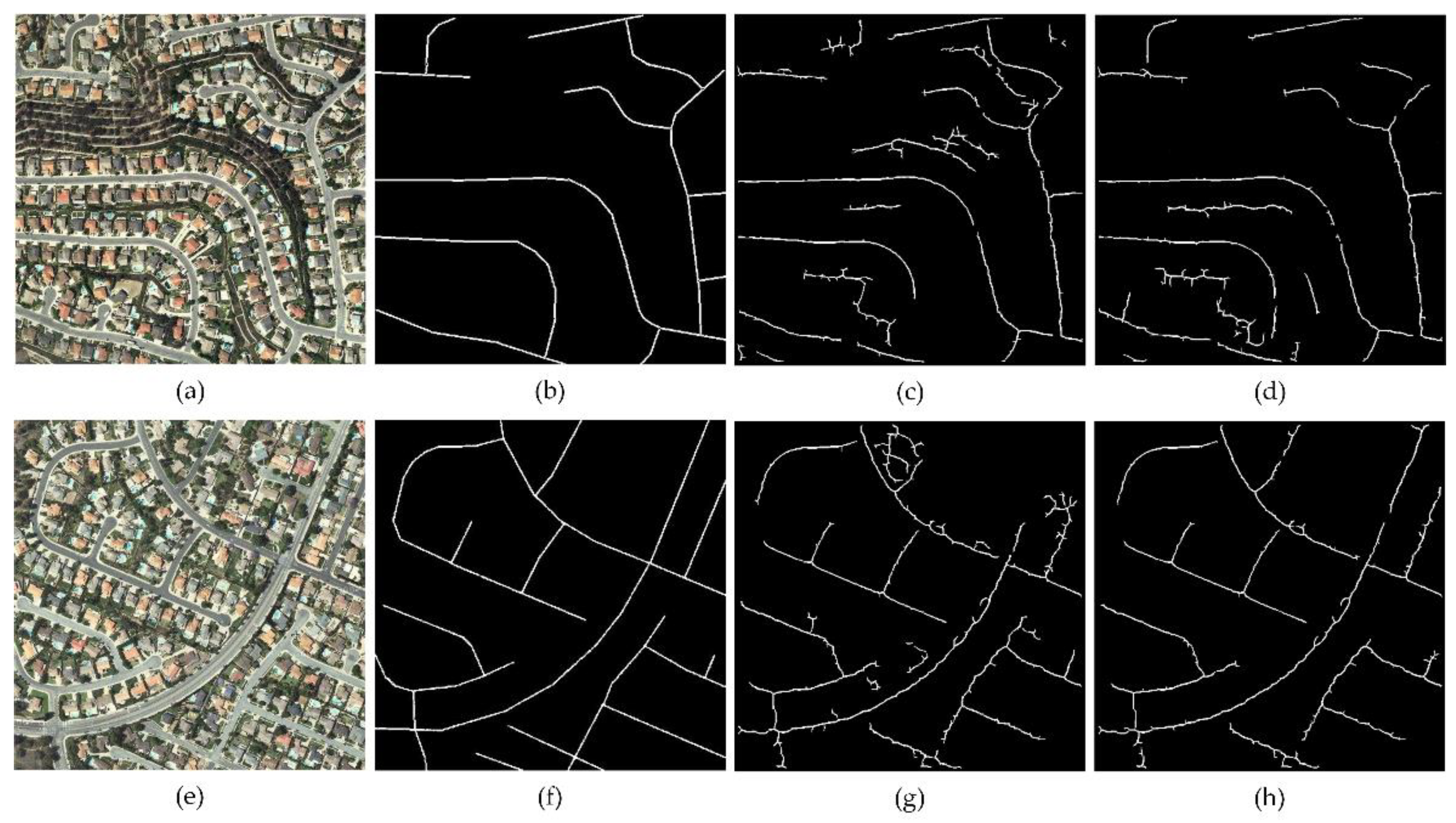
We implemented the method proposed by Lei et al. [26] to prove the superiority of this method in an urban area. The test satellite images were downloaded from VPLab [40]. Figure 12a,e shows the two original images in the urban area. Figure 12b,f shows road-vector data from manual acquisition. The result obtained by the algorithm of Lei et al. is shown in Figure 12c,g, and the result by the proposed method is shown in Figure 12d,h. Table 3 shows the performance of the two methods.
As is shown in Table 3, the two methods both performed well in terms of completeness. Methods based on region analysis are effective in dealing with scenes where the road surface has spectral consistency, like Images I and II. However, the method of Lei et al. showed relatively poor performance for correctness and quality, and the causative faults suggest similar spectral representation of the targets and backgrounds and an incomplete road-tracking mean. The proposed method applies edge constraints to obtain a more stable segmentation result and uses additional, well-behaved shape features to track road objects. The final results indicate the validity.
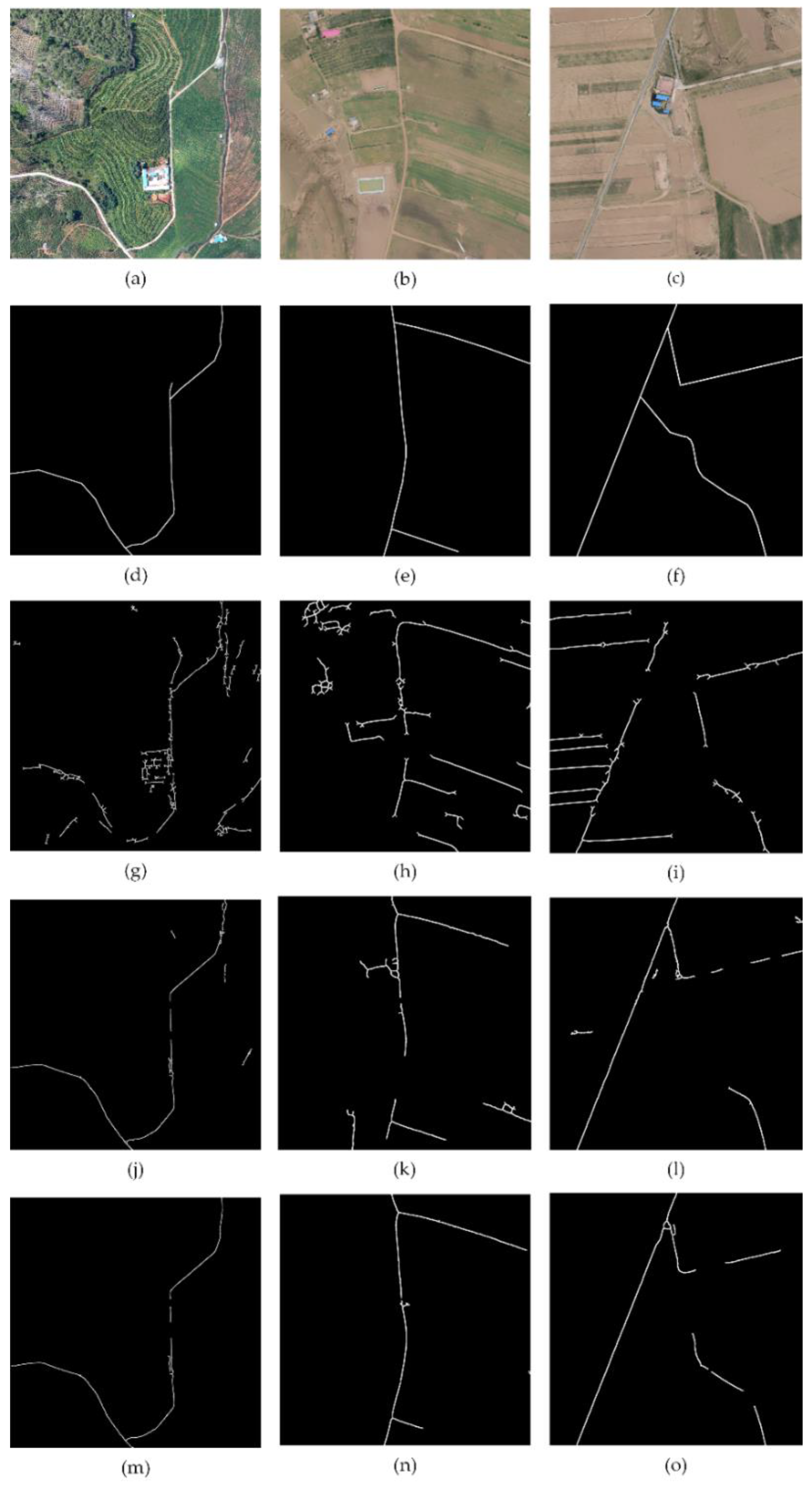
To further prove the superiority of the method, we chose three test images in consideration of the problems discussed in Section 2, such as shadows or shelters of trees and buildings, similar spectral representation of target objects to the backgrounds, and disturbances or shelters on the road surface. Figure 13a is an original aerial image of a rural part of Panzhihua City, China, with a spatial dimension of 2500 × 2500 pixels and a spatial resolution 0.1 m per pixel, while Figure 13b,c shows the original aerial images of rural parts of Dingbian County, China, with a spatial dimension of 1500 × 1500 pixels and a spatial resolution 0.4 m per pixel. We compared the proposed method with the methods of Zang et al. [19] and Lei et al. [26], and Table 4 shows the performance.
We can see that the method of Zang et al. performed well in terms of completeness in Images I and III, which proves the validity of combining canny edge and edge mask constructed by ADSM. However, in Image II, where the road edge is not so conspicuous, the Zang et al. method was not quite complete on account of its weakness in detecting weak edges. The method of Lei et al. performed well when the road surface had spectral consistency, such as the scenes in Images I and II, but lost completeness when the road surface was sheltered. The proposed algorithm returned better results. This can be ascribed to the properties of Gabor filters being sensitive to variations of texture information, allowing them to detect relatively weak edges, and the connection analysis for detected Gabor features also complements the completeness of edge information. The information was used as edge constraints for spectral segmentation.
In terms of correctness and quality, the method of Zang et al. performed quite poorly on account of, on the one hand, its inability to distinguish interferential edges that possess roadlike spatial characteristics from road regions, and, on the other hand, the superfluous information in VHR imagery. The method of Lei et al. showed better correctness and quality in VHR imagery because more pixels on the road surface were available for spectral analysis. However, this method relies too much on spectral information, resulting in false positives and negatives when targets and backgrounds possess similar spectral representations. The proposed method, however, could exploit the superiority of both the spectral and edge characteristics and could separate some roadside artifacts or shadows of trees and buildings from road regions to obtain more stable segmentation results. The final results proved its validity.
In terms of extraction efficiency, Table 5 lists the processing time for the three algorithms. Normally, for an image size of 5001 × 5001, the method of Zang et al. requires 2–10 min to process, the method of Lei et al. takes less than 1 min, and the proposed method takes about 50–80 s. Compared to the Lei et al. method, in which the extra time is mainly consumed by edge-feature analysis, the proposed method has proven to be efficient in accurate road-object extraction when processing VHR remote-sensing images.
4. Conclusions
It is common to find nontarget objects mixed up with road regions due to the great complexity of VHR images. In this paper, a method to efficiently extract accurate road regions from VHR remote-sensing imagery was proposed. To exploit both spatial and spectral information, the method used connected Gabor features as edge constraints for subsequent object segmenting and the region-growing process. Edge constraints with favorable completeness proved to be valid in helping to separate road objects from numerous disturbances. The segmenting results demonstrate the superiority of this method to quickly acquire stable segmented objects while abandoning superfluous pixels with confused uncertainty under the principle of putting quality before quantity. In such VHR images, there are sufficient pixels with great stability for road-object tracking, in which road-object extraction by shape features performs well at keeping false negatives while eliminating false positives. Despite the outstanding performance of this method, further studies are needed to realize higher extraction efficiency with high extraction accuracy. The limitations of the method can be ascribed to the following:
• Lacking rigorous determination of thresholds in Gabor detection and region segmentation.
For various complex scenes, there are discrepancies in the responses of road edges to Gabor filters that cause difficulties for the automatic decision of the response threshold. Despite, in most cases, an approximately precise threshold ST in region segmentation being enough to obtain the desired segmentation result, this sometimes causes severe loss of road information when ST is relatively too small, and undesirable error extraction when ST is too large.
• Nonautomatic determination of optimum scales range.
In this study, the optimum scale range was determined subjectively by experimentally checking Gabor feature-detection results. A systematic method to automatically determine optimum scale ranges that could highlight objects of interest is needed. The determination of the scale can be affected by the resolution of the imagery set and the type of road.
• Unsatisfactory performance in connecting winding Gabor features.
Our method for Gabor features connection is line-segment based. For curved-road parts that are missing much edge information, it is difficult to complement the edge by simply using the connection stratagem of this article. Further studies for recognizing and fitting curved roads are necessary.
Author Contributions
L.C. developed the methodology and the system. Ideas, considerations and discussion of the work were supervised by Q.Z. X.X. provided technique support and contributed to the paper writing. H.H. contributed to the experimental study and gave some novel ideas. And H.Z. contributed to the revision of the paper.
Funding
This research was funded by National Natural Science Foundation of China under Grant Nos. 41631174 and No. 41701466.
References
- Fortier, A.; Ziou, D.; Armenakis, C.; Wang, S. Survey of Work on Road Extraction in Aerial and Satellite Images; Technical Report; Center for Topographic Information Geomatics: Ontario, ON, Canada, 1999. [Google Scholar]
- Memon, I.; Chen, L.; Majid, A.; Lv, M.; Hussain, I.; Chen, G. Travel recommendation using geo-tagged photos in social media for tourist. Wirel. Pers. Commun. 2015, 80, 1347–1362. [Google Scholar] [CrossRef]
- Shifa, A.; Afgan, M.S.; Asghar, M.N.; Fleury, M.; Memon, I.; Abdullah, S.; Rasheed, N. Joint crypto-stego scheme for enhanced image protection with nearest-centroid clustering. IEEE Access 2018, 6, 16189–16206. [Google Scholar] [CrossRef]
- Memon, I.; Chen, L.; Arain, Q.A.; Memon, H.; Chen, G. Pseudonym changing strategy with multiple mix zones for trajectory privacy protection in road networks. Int. J. Commun. Syst. 2018, 31, e3437. [Google Scholar] [CrossRef]
- Gao, L.; Shi, W.; Miao, Z.; Lv, Z. Method based on edge constraint and fast marching for road centerline extraction from very high-resolution remote sensing images. Remote Sens. 2018, 10, 900. [Google Scholar] [CrossRef]
- Demir, I.; Koperski, K.; Lindenbaum, D.; Pang, G.; Huang, J.; Basu, S.; Hughes, F.; Tuia, D.; Raskar, R. Deepglobe 2018: A challenge to parse the earth through satellite images. arXiv, 2018; arXiv:1805.06561. [Google Scholar]
- Shi, W.; Miao, Z.; Debayle, J. An integrated method for urban main-road centerline extraction from optical remotely sensed imagery. IEEE Trans. Geosci. Remote Sens. 2014, 52, 3359–3372. [Google Scholar] [CrossRef]
- Poullis, C.; You, S. Delineation and geometric modeling of road networks. ISPRS J. Photogramm. Remote Sens. 2010, 65, 165–181. [Google Scholar] [CrossRef]
- Wei, Y.; Wang, Z.; Xu, M. Road structure refined cnn for road extraction in aerial image. IEEE Geosci. Remote Sens. Lett. 2017, 14, 709–713. [Google Scholar] [CrossRef]
- Buslaev, A.; Seferbekov, S.S.; Iglovikov, V.I.; Shvets, A.A. Fully convolutional network for automatic road extraction from satellite imagery. arXiv, 2018; arXiv:1806.05182. [Google Scholar]
- Alshehhi, R.; Marpu, P.R.; Woon, W.L.; Dalla Mura, M. Simultaneous extraction of roads and buildings in remote sensing imagery with convolutional neural networks. ISPRS J. Photogramm. Remote Sens. 2017, 130, 139–149. [Google Scholar] [CrossRef]
- Canny, J. A computational approach to edge detection. IEEE Trans. Pattern Anal. Mach. Intell. 1986, 679–698. [Google Scholar] [CrossRef]
- Von Gioi, R.G.; Jakubowicz, J.; Morel, J.-M.; Randall, G. Lsd: A fast line segment detector with a false detection control. IEEE Trans. Pattern Anal. Mach. Intell. 2010, 32, 722–732. [Google Scholar] [CrossRef] [PubMed]
- Zang, Y.; Wang, C.; Yu, Y.; Luo, L.; Yang, K.; Li, J. Joint enhancing filtering for road network extraction. IEEE Trans. Geosci. Remote Sens. 2017, 55, 1511–1525. [Google Scholar] [CrossRef]
- Kaur, S.; Baghla, S. Automatic road detection of satellite images using improved edge detection. Int. J. Comput. Technol. 2013, 10, 1546–1552. [Google Scholar] [CrossRef]
- Liu, W.; Zhang, Z.; Chen, X.; Li, S.; Zhou, Y. Dictionary learning-based hough transform for road detection in multispectral image. IEEE Geosci. Remote Sens. Lett. 2017, 14, 2330–2334. [Google Scholar] [CrossRef]
- Shao, Y.; Guo, B.; Hu, X.; Di, L. Application of a fast linear feature detector to road extraction from remotely sensed imagery. IEEE J. Sel. Top. Appl. Earth Obs. Remote Sens. 2011, 4, 626–631. [Google Scholar] [CrossRef]
- Lisini, G.; Tison, C.; Cherifi, D.; Tupin, F.; Gamba, P. Improving Road Network Extraction in High-Resolution sar Images by Data Fusion. Presented at CEOS SAR Workshop, Ulm, Germany, 27–28 May 2004. [Google Scholar]
- Zang, Y.; Wang, C.; Cao, L.; Yu, Y.; Li, J. Road network extraction via aperiodic directional structure measurement. IEEE Trans. Geosci. Remote Sens. 2016, 54, 3322–3335. [Google Scholar] [CrossRef]
- Yuan, J.; Tang, S.; Wang, F.; Zhang, H. A robust road segmentation method based on graph cut with learnable neighboring link weights. In Proceedings of the 17th International IEEE Conference on Intelligent Transportation Systems (ITSC), Qingdao, China, 8–11 October 2014; pp. 1644–1649. [Google Scholar]
- Akram, K.M.; Elahi, M.M.L.; Amin, M.A. Multiple level set region based single line road extraction. In Proceedings of the 2013 International Conference on Machine Learning and Cybernetics, Tianjin, China, 14–17 July 2013; pp. 1201–1206. [Google Scholar]
- Gaetano, R.; Masi, G.; Poggi, G.; Verdoliva, L.; Scarpa, G. Marker-controlled watershed-based segmentation of multiresolution remote sensing images. IEEE Trans. Geosci. Remote Sens. 2015, 53, 2987–3004. [Google Scholar] [CrossRef]
- Song, M.; Civco, D. Road extraction using svm and image segmentation. Photogramm. Eng. Remote Sens. 2004, 70, 1365–1371. [Google Scholar] [CrossRef]
- Maboudi, M.; Amini, J.; Hahn, M.; Saati, M. Object-based road extraction from satellite images using ant colony optimization. Int. J. Remote Sens. 2017, 38, 179–198. [Google Scholar] [CrossRef]
- Shi, W.; Miao, Z.; Wang, Q.; Zhang, H. Spectral-spatial classification and shape features for urban road centerline extraction. IEEE Geosci. Remote Sens. Lett. 2014, 11, 788–792. [Google Scholar]
- Xiaoqi, L.; Weixing, W.; Jun, L. A method of road extraction from high-resolution remote sensing images based on shape features. Acta Geod. Cartogr. Sin. 2016, 38, 457–465. [Google Scholar]
- Kumar, M.; Singh, R.; Raju, P.; Krishnamurthy, Y. Road network extraction from high resolution multispectral satellite imagery based on object oriented techniques. ISPRS Ann. Photogramm. Remote Sens. Spat. Inf. Sci. 2014, 2, 107. [Google Scholar] [CrossRef]
- Memon, M.H.; Li, J.-P.; Memon, I.; Arain, Q.A. Geo matching regions: Multiple regions of interests using content based image retrieval based on relative locations. Multimed. Tools Appl. 2017, 76, 15377–15411. [Google Scholar] [CrossRef]
- Memon, M.H.; Li, J.-P.; Memon, I.; Shaikh, R.A.; Mangi, F.A. Efficient object identification and multiple regions of interest using cbir based on relative locations and matching regions. In Proceedings of the 2015 12th International Computer Conference on Wavelet Active Media Technology and Information Processing (ICCWAMTIP), Chengdu, China, 18–20 December 2015; pp. 247–250. [Google Scholar]
- Alshehhi, R.; Marpu, P.R. Hierarchical graph-based segmentation for extracting road networks from high-resolution satellite images. ISPRS J. Photogramm. Remote Sens. 2017, 126, 245–260. [Google Scholar] [CrossRef]
- Zhao, W.; Luo, L.; Guo, Z.; Yue, J.; Yu, X.; Liu, H.; Wei, J. Road extraction in remote sensing images based on spectral and edge analysis. Guang Pu Xue Yu Guang Pu Fen Xi= Guang Pu 2015, 35, 2814–2819. [Google Scholar] [PubMed]
- Daugman, J.G. Uncertainty relation for resolution in space, spatial frequency, and orientation optimized by two-dimensional visual cortical filters. JOSA A 1985, 2, 1160–1169. [Google Scholar] [CrossRef]
- Kamarainen, J.-K.; Kyrki, V.; Kalviainen, H. Invariance properties of gabor filter-based features-overview and applications. IEEE Trans. Image Process. 2006, 15, 1088–1099. [Google Scholar] [CrossRef] [PubMed]
- Kamarainen, J.-K. Gabor features in image analysis. In Proceedings of the 2012 3rd International Conference on Image Processing Theory, Tools and Applications (IPTA), Istanbul, Turkey, 15–18 October 2012; pp. 13–14. [Google Scholar]
- Ilonen, J.; Kamarainen, J.-K.; Kalviainen, H. Fast extraction of multi-resolution gabor features. In Proceedings of the 14th International Conference on Image Analysis and Processing (ICIAP 2007), Modena, Italy, 10–14 September 2007; pp. 481–486. [Google Scholar]
- Sghaier, M.O.; Lepage, R. Road extraction from very high resolution remote sensing optical images based on texture analysis and beamlet transform. IEEE J. Sel. Top. Appl. Earth Obs. Remote Sens. 2016, 9, 1946–1958. [Google Scholar] [CrossRef]
- Shaikh, R.A.; Deep, S.; Li, J.-P.; Kumar, K.; Khan, A.; Memon, I. Contemporary integration of content based image retrieval. In Proceedings of the 2014 11th International Computer Conference on Wavelet Actiev Media Technology and Information Processing(ICCWAMTIP), Chengdu, China, 19–21 December 2014; pp. 301–304. [Google Scholar]
- Memon, M.H.; Khan, A.; Li, J.-P.; Shaikh, R.A.; Memon, I.; Deep, S. Content based image retrieval based on geo-location driven image tagging on the social web. In Proceedings of the 2014 11th International Computer Conference on Wavelet Actiev Media Technology and Information Processing(ICCWAMTIP), Chengdu, China, 19–21 December 2014; pp. 280–283. [Google Scholar]
- Liu, J.; Qin, Q.; Li, J.; Li, Y. Rural road extraction from high-resolution remote sensing images based on geometric feature inference. ISPRS Int. J. Geo Inf. 2017, 6, 314. [Google Scholar] [CrossRef]
- VPLab Data. Available online: http://www.cse.iitm.ac.in/~vplab/satellite.html (accessed on 16 April 2017).
Figure 1.
Flowchart of the proposed method.
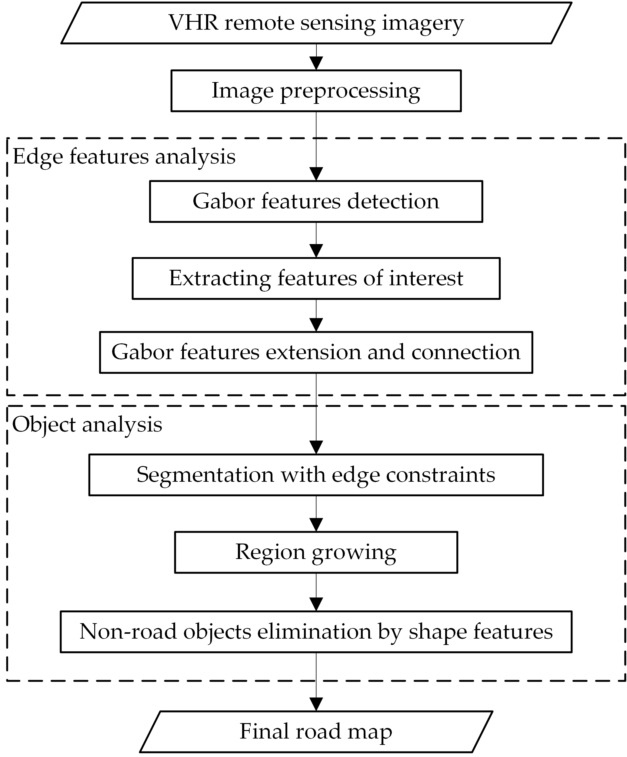
Figure 2.
(a–h) .
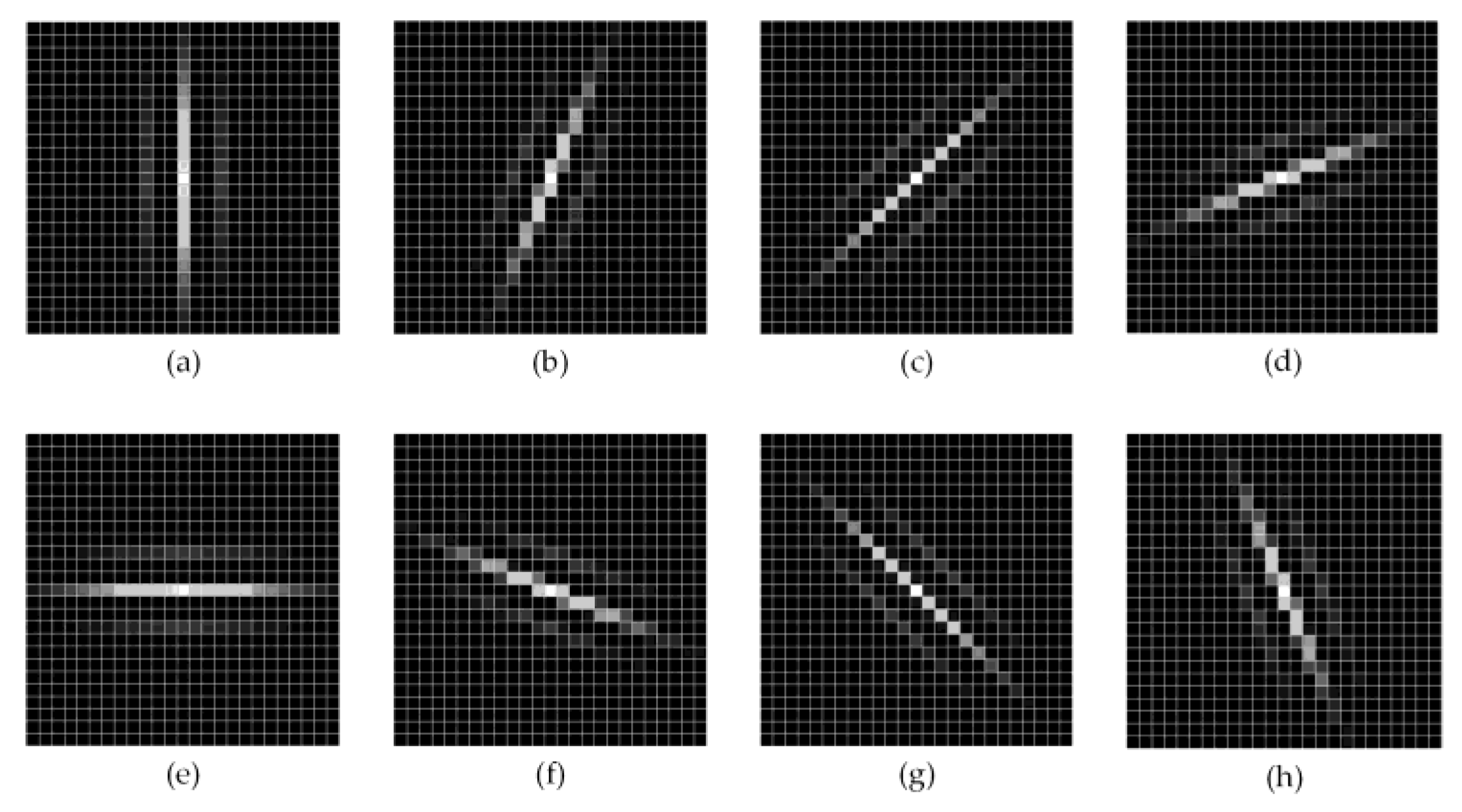
Figure 3.
Extraction of Gabor features of interest. (a) Original map with many disturbances; (b) map of merged Gabor features; (c) merged map of Gabor features of interest in each orientation.
Figure 3.
Extraction of Gabor features of interest. (a) Original map with many disturbances; (b) map of merged Gabor features; (c) merged map of Gabor features of interest in each orientation.
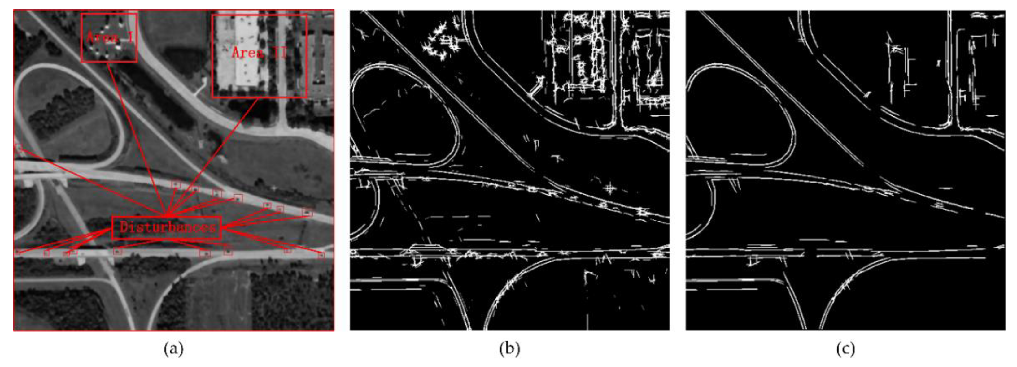
Figure 4.
Edge-detection comparison. (a,d) Original image where edge information is not so conspicuous; (b,e) result by canny algorithm, lower- and upper-threshold parameters were set to 50 and 100, respectively; (c,f) erged map by eight orientation filter results (, , , ).
Figure 4.
Edge-detection comparison. (a,d) Original image where edge information is not so conspicuous; (b,e) result by canny algorithm, lower- and upper-threshold parameters were set to 50 and 100, respectively; (c,f) erged map by eight orientation filter results (, , , ).

Figure 5.
Sketch map for line segment pair connection.
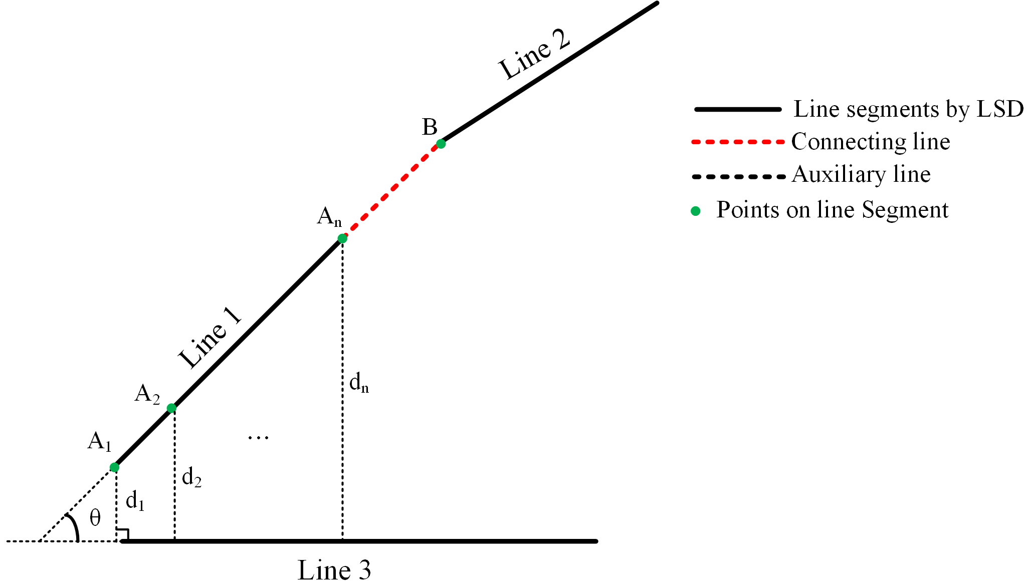
Figure 6.
Edge constraints. (a) Original map where target road mixes with houses; (b) Gabor features by line-segment detection (LSD) analysis; (c) connection analysis; (d) segmentation with edge constraints.
Figure 6.
Edge constraints. (a) Original map where target road mixes with houses; (b) Gabor features by line-segment detection (LSD) analysis; (c) connection analysis; (d) segmentation with edge constraints.
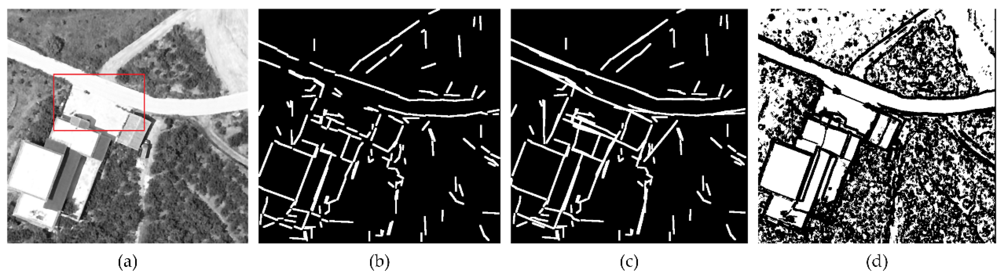
Figure 7.
Neighbor pixels within ΔD.

Figure 8.
(a) Original map; (b) segmentation results of the method by Gaetano et al. [22]; (c) segmentation results of our proposed method.
Figure 8.
(a) Original map; (b) segmentation results of the method by Gaetano et al. [22]; (c) segmentation results of our proposed method.

Figure 9.
Center point at the edge of the object.

Figure 10.
(a) Straight-road-object model; (b) curved-road-object model.

Figure 11.
(a) Original image; (b) preprocessed grayscale map; (c) merged Gabor features in best scale; (d) connected Gabor features of interest; (e) object segmentation with edge constraints; (f) region-growing result; (g) road-object tracking by shape features; (h) skeleton extraction.
Figure 11.
(a) Original image; (b) preprocessed grayscale map; (c) merged Gabor features in best scale; (d) connected Gabor features of interest; (e) object segmentation with edge constraints; (f) region-growing result; (g) road-object tracking by shape features; (h) skeleton extraction.

Figure 12.
Comparison of the method of Lei et al. [26] and the proposed method in an urban area; (a,e) original image; (b,f) road-vector data from manual acquisition; (c,g) results of the method of Lei et al.; (d,h) results of proposed method.
Figure 12.
Comparison of the method of Lei et al. [26] and the proposed method in an urban area; (a,e) original image; (b,f) road-vector data from manual acquisition; (c,g) results of the method of Lei et al.; (d,h) results of proposed method.

Figure 13.
Comparison of the method of Zang et al. [19], Lei et al. [26], and the proposed method in a rural area. (a–c) Original image. (d–f) Road-vector data from manual acquisition. (g–i) Results of the method of Zang et al. (j–l) Results of the method of Lei et al. (m–o) Results of proposed method.


Table 1.
Parameter setting for Gabor wavelets.
| λ | σ | θ | φ | κ |
|---|---|---|---|---|
| λ1 = 2.2 | σ1 = 1.2 | θn = nπ/8, n = 0, 1, 2, …, 7 | φ = 0 | κ = 0.3 |
| λ2 = 3.0 | σ2 = 1.7 | |||
| λ3 = 4.2 | σ3 = 2.4 |
Table 2.
Shape-feature threshold setting for road tracking.
| Road Shape | Area S | Shortest Inner Diameter D | Complex Rate C | Length–Width Ratio of Bounding Rectangle R | Fullness Ratio F |
|---|---|---|---|---|---|
| Straight Line | 1000–50,000 | 30–50 | 100 | 3.5 | - |
| Curve Line | 1000–50,000 | 30–50 | 100 | - | 0.33 |
Table 3.
Performance of the two road-extraction methods.
| Method | Image I | Image II | ||||
|---|---|---|---|---|---|---|
| Completeness | Correctness | Quality | Completeness | Correctness | Quality | |
| Lei et al. [26] | 0.9 | 0.71 | 0.66 | 0.89 | 0.86 | 0.77 |
| -proposed | 0.92 | 0.79 | 0.74 | 0.94 | 0.96 | 0.91 |
Table 4.
Performance of the three road-extraction methods.
| Evaluation | Zang et al. [19] | Lei et al. [26] | Proposed |
|---|---|---|---|
| Image I | |||
| Completeness | 0.89 | 0.97 | 0.97 |
| Correctness | 0.47 | 0.86 | 0.97 |
| Quality | 0.44 | 0.84 | 0.95 |
| Image II | |||
| Completeness | 0.75 | 0.82 | 0.89 |
| Correctness | 0.43 | 0.69 | 0.97 |
| Quality | 0.38 | 0.6 | 0.87 |
| Image III | |||
| Completeness | 0.8 | 0.7 | 0.77 |
| Correctness | 0.47 | 0.92 | 0.96 |
| Quality | 0.42 | 0.66 | 0.75 |
Table 5.
Time consumption of the three methods.
| Method | Implementation Environment | Running Time for Image I | Running Time for Image II | Running Time for Image III |
|---|---|---|---|---|
| Zang et al. [19] | 2.6 GHz Intel Core i7-6700HQ CPU | 271 s | 335 s | 339 s |
| Lei et al. | 2.6 GHz Intel Core i7-6700HQ CPU | 38 s | 47 s | 56 s |
| Proposed | 2.6 GHz Intel Core i7-6700HQ CPU | 49 s | 62 s | 71 s |
© 2018 by the authors. Licensee MDPI, Basel, Switzerland. This article is an open access article distributed under the terms and conditions of the Creative Commons Attribution (CC BY) license (http://creativecommons.org/licenses/by/4.0/).
Share and Cite
MDPI and ACS Style
Chen, L.; Zhu, Q.; Xie, X.; Hu, H.; Zeng, H. Road Extraction from VHR Remote-Sensing Imagery via Object Segmentation Constrained by Gabor Features. ISPRS Int. J. Geo-Inf. 2018, 7, 362. https://doi.org/10.3390/ijgi7090362
AMA Style
Chen L, Zhu Q, Xie X, Hu H, Zeng H. Road Extraction from VHR Remote-Sensing Imagery via Object Segmentation Constrained by Gabor Features. ISPRS International Journal of Geo-Information. 2018; 7(9):362. https://doi.org/10.3390/ijgi7090362
Chicago/Turabian StyleChen, Li, Qing Zhu, Xiao Xie, Han Hu, and Haowei Zeng. 2018. "Road Extraction from VHR Remote-Sensing Imagery via Object Segmentation Constrained by Gabor Features" ISPRS International Journal of Geo-Information 7, no. 9: 362. https://doi.org/10.3390/ijgi7090362
Note that from the first issue of 2016, this journal uses article numbers instead of page numbers. See further details here.