Exploring Railway Network Dynamics in China from 2008 to 2017


1
School of Architecture and Urban Planning, Huazhong University of Science and Technology, Wuhan 430074, China
2
Hubei Engineering and Technology Research Center of Urbanization, Wuhan 430074, China
3
School of Geography and Tourism, Shaanxi Normal University, Xi’an 710119, China
4
Geomatics Technology and Application key Laboratory of Qinghai Province, Xining 810001, China
5
National & Local Joint Engineering Research Center of Geo-spatial Information Technology, Fuzhou University, Fuzhou 350002, China
6
Key Laboratory of Spatial Data Mining & Information Sharing of MOE, Fuzhou 350002, China
*
Author to whom correspondence should be addressed.
ISPRS Int. J. Geo-Inf. 2018, 7(8), 320; https://doi.org/10.3390/ijgi7080320
Submission received: 10 July 2018
/
Revised: 3 August 2018
/
Accepted: 7 August 2018
/
Published: 8 August 2018
Abstract
:China’s high speed rail (HSR) network has been rapidly constructed and developed during the past 10 years. However, few studies have reported the spatiotemporal changes of railway network structures and how those structures have been affected by the operation of high speed rail systems in different periods. This paper analyzes the evolving network characteristics of China’s railway network during each of the four main stages of HSR development over a 10-year period. These four stages include Stage 1, when no HSR was in place prior to August 2008; Stage 2, when several HSR lines were put into operation between August 2008, and July 2011; Stage 3, when the network skeleton of most main HSR lines was put into place. This covered the period until January 2013. Finally, Stage 4 covers the deep intensification of several new HSR lines and the rapid development of intercity-HSR railway lines between January 2013, and July 2017. This paper presents a detailed analysis of the timetable-based statistical properties of China’s railway network, as well as the spatiotemporal patterns of the more than 2700 stations that have been affected by the opening of HSR lines and the corresponding policy changes. Generally, we find that the distribution of both degrees and strengths are characterized by scale-free patterns. In addition, the decreasing average path length and increasing network clustering coefficient indicate that the small world characteristic is more significant in the evolution of China’s railway network. Correlations between different network indices are explored, in order to further investigate the dynamics of China’s railway system. Overall, our study offers a new approach for assessing the growth and evolution of a real railway network based on train timetables. Our study can also be referenced by policymakers looking to adjust HSR operations and plan future HSR routes.
1. Introduction
Railway networks play an indispensable and essential role in public transportation systems all around the world, due to their high efficiency and convenience [1,2]. For instance, the total mileage of China’s rail lines is approximately 670 thousand kilometers, which ranks second in the world [3]. Moreover, according to the 2017 China Statistical Yearbook, the passenger volume of railway transport during that year exceeded 2.8 billion, which is 3.7 times the combined total of passengers who travelled by water and civil aviation transport [4]. As one of the most populous countries in the world, the past decade has witnessed the increasing pace of China’s high-speed rail (HSR) network construction and rapid development.
Many studies have focused on the effects of high speed rail systems in many countries. These studies have examined such issues as improving urban accessibility [5,6,7], and extending the accessibility gap between major cities and small and medium-sized cities [8,9], polarization traffic [10,11], improving the environmental quality [12,13], strengthening economic relationships between cities [5,13,14], changing the characteristics of urban spatial patterns, and many other effects [15,16]. In addition, Cao et al. quantified the average travel time, travel cost and other indicators of major cities along China’s high speed rail network [5]. This study found that cities with higher population and which are more economically developed benefit more from HSR. Shaw et al. established a railway transfer model and analyzed the changes in time accessibility of all cities served by China’s railway system, under the influences of HSR [6]. They found that the impact of HSR differs from region to region (in terms of in-vehicle time and out-of-vehicle time) [6]. However, existing studies lack any detailed analysis of the evolving characteristics of railway networks under the influence of HSR.
Understanding traffic network structures and their complexity is an important issue in the fields of traffic, geography and computing science [17,18,19]. Fortunately, the development of network science has provided a new special perspective for understanding the complexity of networks in both physical and virtual space [20,21]. A large number of empirical studies have been conducted using complex network theory for railway networks [22,23], aviation networks [24,25] and maritime networks [26,27] from a global to a national level. In addition, complex network theory has been applied to subway networks [28] and human mobility networks [29,30] at a city level, and social and other networks in virtual space [31,32]. The railway networks in Asia, Europe and North America are well developed and are often used for research (especially in China, India and other populous countries). For example, Sen discovered that the India railway network (IRN) has small world characteristics [22]. In addition, Ghosh et al. found that the distribution of nodes in the India railway network follows exponential law [33]. The study further extracted the important stations in IRN based on connectivity and traffic flow. Li and Cai found that the decay of node degree and strength distribution follows the power law in China’s static railway network [23]. This is different from the exponential law of India’s railway network. However, the railway networks used in the abovementioned studies are mostly static. Few studies have reported on the spatiotemporal changes of railway network structures affected by the operation of HSR in different periods. Moreover, the network data used in some studies are not complete. For example, only express train routes were used to analyze the IRN structure [33]. In addition, Lin et al. only used airline data from a statistical yearbook. This method would create the representativeness problem of spatial sampling and also ignore the role of small and medium cities in the whole network [24]. This article analyzes all the cities served by China’s railway system, and our analysis results also involve small and medium-sized cities.
The past ten years have witnessed the rapid construction and development of China’s high-speed rail network. The dynamic complexity and spatial expansion of China’s railway network is unprecedented. According to the “National medium and long-term railway network plan” released by the State Council of the People’s Republic of China in 2004, the first HSR line (the Beijing-Tianjin intercity HSR) was opened on 1 August 2008. The operational length of China’s HSR had reached 9300 km by the end of 2012 [4]. In addition, in the process of rapid construction, the operational policies were constantly being adjusted and changed. This affected, areas such as speed reduction, ticket price reduction, rearrangement of train timetables, etc. Together, this all led to the unique and special mechanism and topological structure of China’s railway network. However, there has been very little investigation into how the implementation and regulation of these policies and mechanisms has impacted on China’s HSR and the evolving timetable-based network characteristics. In the contexts described above, exploring the evolving network characteristics of China’s railway system is of the utmost interest and importance to researchers and policy-makers.
Therefore, this paper divides the development of China’s railway system over the past 10 years into four main stages. We investigate the evolution of China’s railway network, composed of more than 2700 stations, from a complex network perspective. The weight matrixes between each city are derived from the Chinese railway timetables for each of the four stages. The contributions of this study are two-fold. Firstly, different from the perspective of geographic space, this paper analyzes the evolution of China’s railway network under the impacts of HSR over the past 10 years, based on the complex network perspective. We further extract the hub-and-spoke structure of China’s railway network through the correlation analysis between network indices, and we put forward suggestions for constructing railway networks and selecting railway hubs. Secondly, different from passenger volume data in the statistical yearbook, the train timetable is very important to train operations [34]. This article uses train timetable data during the four different stages as a means to analyze the evolution of China’s railway network. Not only is the data easy to obtain, but policy effects can also be merged into the analysis. This is of great importance to the optimization of the national train timetable, as well as the response of operational policies.
The remaining parts of this study are organized as follows: Section 2 gives a brief introduction to the development of China’s railway system during the past decade. Section 3 introduces the acquisition of train timetable dataset, and the modeling of railway network in this paper. Section 4 discusses the results. Section 5 summarizes the findings and discusses future research directions.
2. Development of China’s Railway System from 2008–2017
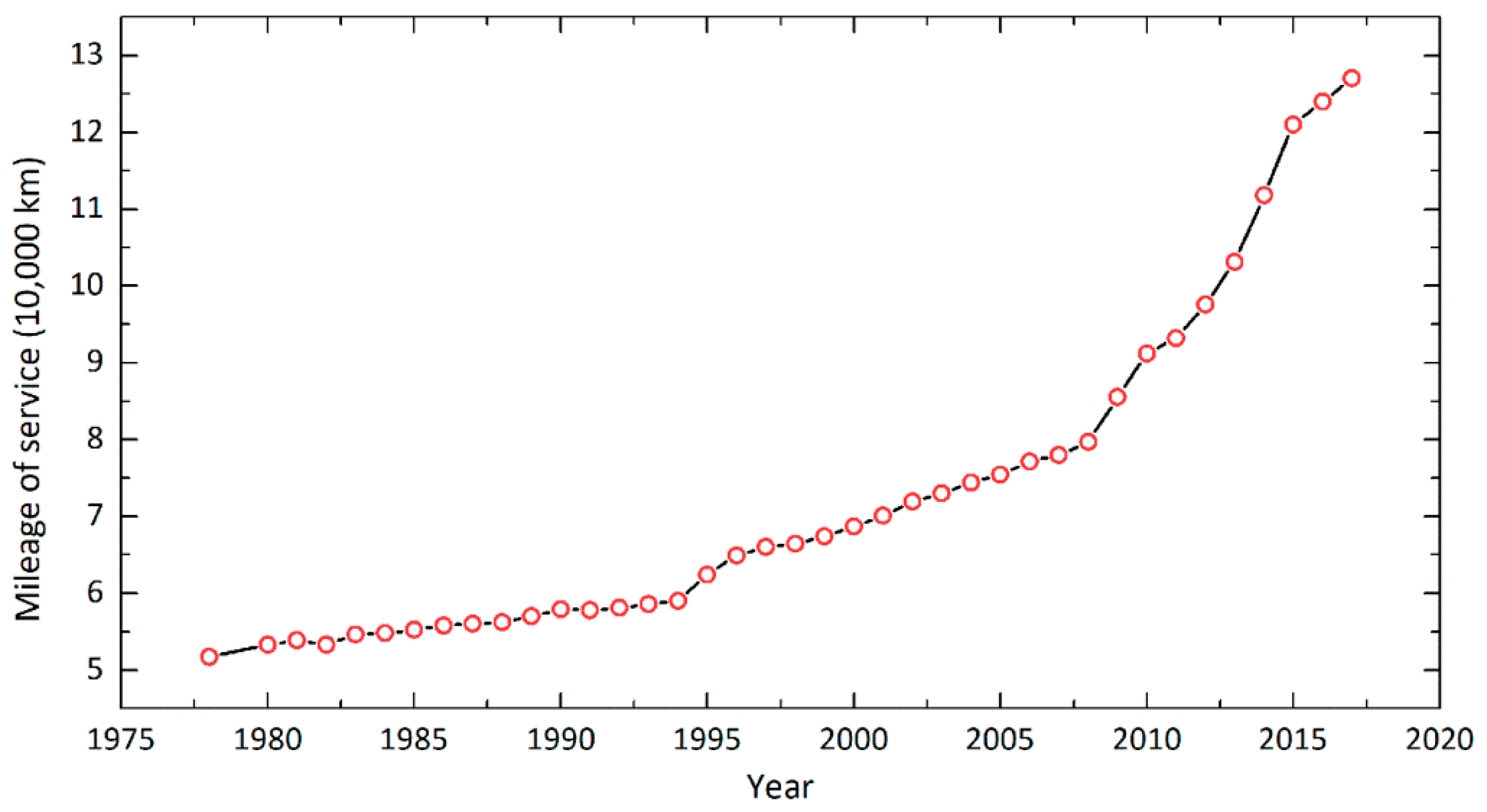
It has been more than 120 years since the first railway line was built in China in 1876. After 1978, China’s railway system entered a stage of scientific development. Wang et al. provided a detailed introduction to the development of Chinese railways before 2000 [1]. In 2004, the State Council of the People’s Republic of China released the “National medium and long-term railway network plan”. This document was intended to guide the development and construction of China’s railway system, and especially the HSR network. This plan was initially implemented in 2008. According to this plan, China will construct at least eight, main horizontal and vertical HSR lines with a total length of over 12,000 km. These lines will provide a HSR passenger route network during the coming decades. Sixteen high-speed rail lines (eight horizontal and eight vertical) interweave vertically and horizontally, forming a huge traffic network that will cover more than 80% of China’s large cities and 90% of the population. The mileage covered by China’s railway network in each year is shown below in Figure 1 [4].
On 1 August 2008, China’s first inter-city HSR (Beijing-Tianjin) train, with world-leading technology and an operating speed of 350 km/h, was opened. In July 2011, the speed reduction policy of China’s HSR was introduced. This policy reduced the speed in areas where 350 km/h had been permitted to 300 km/h; 250 km/h were reduced to 200 km/h, and the national train timetable was rearranged. By the end of 2012, more than 13,000 km of dedicated passenger lines with speeds of 250–350 km/h were completed and put into operation in China. The skeleton of China’s HSR network of “four vertical and four horizontal lines” was basically formed, launching the Chinese railway system into the era of high-speed railways. In January 2013, the Ministry of Railway announced a policy of ticket fare reductions, lowering by 2% the basic train fares. Then, several provincial capital cities increased the rapid development of intercity-HSR (e.g., Guangzhou, Wuhan, Changsha, Chengdu, Zhengzhou). By the end of 2017, the national railway operating mileage had reached 127,000 km. Of that total, the HSR network’s operating length had reached 25,000 km, serving more than 500 cities, which ranks China first in the world.
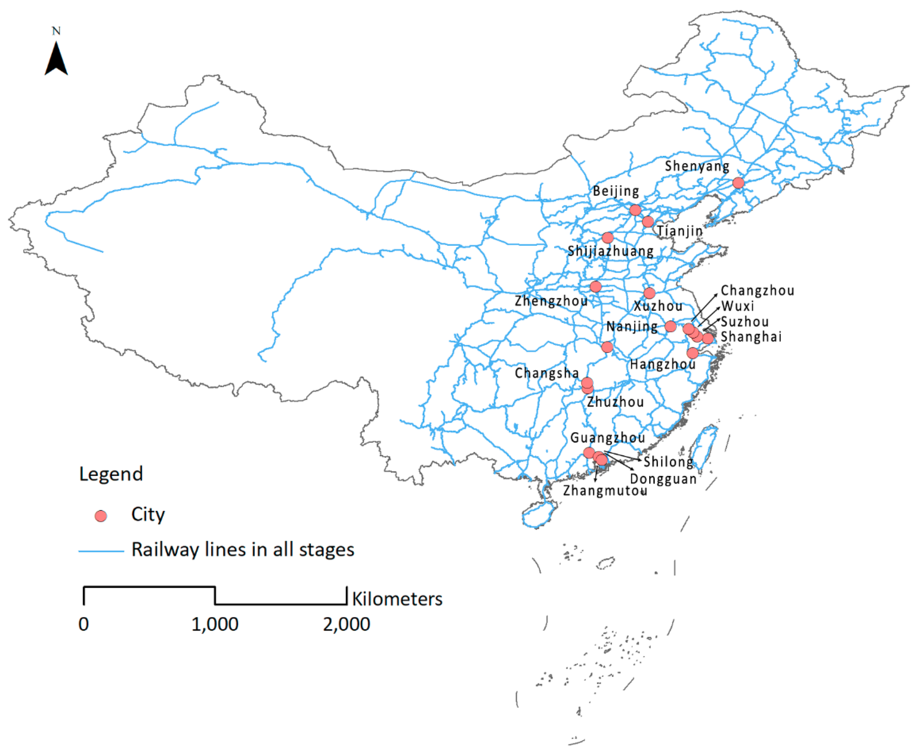
Based on the above information, combined with the increasing mileage of railway lines, as well as the adjustment of China’s operational policies, we have divided the development of China’s railway network into four main stages covering the past 10 years: Stage 1, prior to August 2008, when there was a traditional rail service; Stage 2, between 2008 and 2011, when several HSR lines were put into use; Stage 3, between 2011 and 2013, when there was steady growth in the number of HSR lines, and Stage 4, (after 2013), which has experience the rapid growth of HSR and intercity-HSR lines, as shown in Table 1. The spatial distributions of rail lines during different stages are shown in Figure 2.
3. Data
The data used in this paper are the train operation timetable data covering all four of the above named stages. The train timetable is a form of information that gives the arrival, departure and stop times of each train route at each railway station. Table 2 shows the types and characteristics of passenger trains in China at present (excluding temporary train lines).
In this study, we base our assumptions regarding the building of China’s train line network on the train line timetables released by the Ministry of Railways of the Peoples’ Republic of China. The timetables of all rail lines during the four rail service stages detailed above were captured individually by parsing the online information of an official website (www.12306.cn). The details on this website were released by the Ministry of Railways of the Peoples’ Republic of China. Table 3 gives an example of the timetable of rail line G107. The timetable includes the necessary information including the stations, arrival times, departure times, duration of stop times, distance from the origin station, the lowest ticket fare and so on. The train timetables of each stage are saved in ArcGIS Geodatabase.
At the same time, the latitude and longitude coordinates of all stations and cities have been acquired from Google Maps. Trains in Taiwan, Hong Kong, and Macao are not included in this study.
4. Methodology
In this section, we discuss the methodology used in this study to build a railroad network database, and to compute timetable-based network indices.
4.1. Building a Railroad Network Database
The railroad network (G) is comprised of train stations (V), railroad segments (E) and train routes (R). Each railroad segment is a linkage between two adjacent stations in one train route. There are at least two stations and at least one railroad segment on each train route. When a train route has more than two train stations, that train route is comprised of several railroad segments.
Since there may be more than two stations in one train route, it is imperative to pay extra attention to the generalization method of networks and adjacent matrixes. Thus, in order to derive the timetable-based weight matrix, this paper introduces the P-Spatial graph to process each train route. At present, there are two main models that can be used to transfer the traffic routes into the weighted network, namely the L-space graph and the P-space graph [22,35,36]. In an L-space graph, only two adjacent nodes are considered to be directly connected on a multi-station line. However, in a P-space graph, all nodes connected by the same line are considered to be connected [22], and this graph was used earlier for IRN analysis. Since this study is based on train timetables from a complex network framework, the P-space graph focuses on accessibility and is more appropriate for the transfer analysis used to calculate shortest path length. Thus, a P-space graph is more suitable to the complex network analysis of China’s railway network. Therefore, this paper uses a P-space graph to construct a railway network.
In a weighted HSR network, a node is a named city, and a weight is one segment of the train route. Firstly, the weights between i and j in a network are initialized as Aij = 0. For every train route in the train timetable obtained by the crawler, the specific rule to obtain the weight matrix is as follows:
(1) If two cities i and j can be accessed without any transfer, it is considered that the two nodes are connected to each other, and the corresponding weight aij between i and j is set to plus 1.
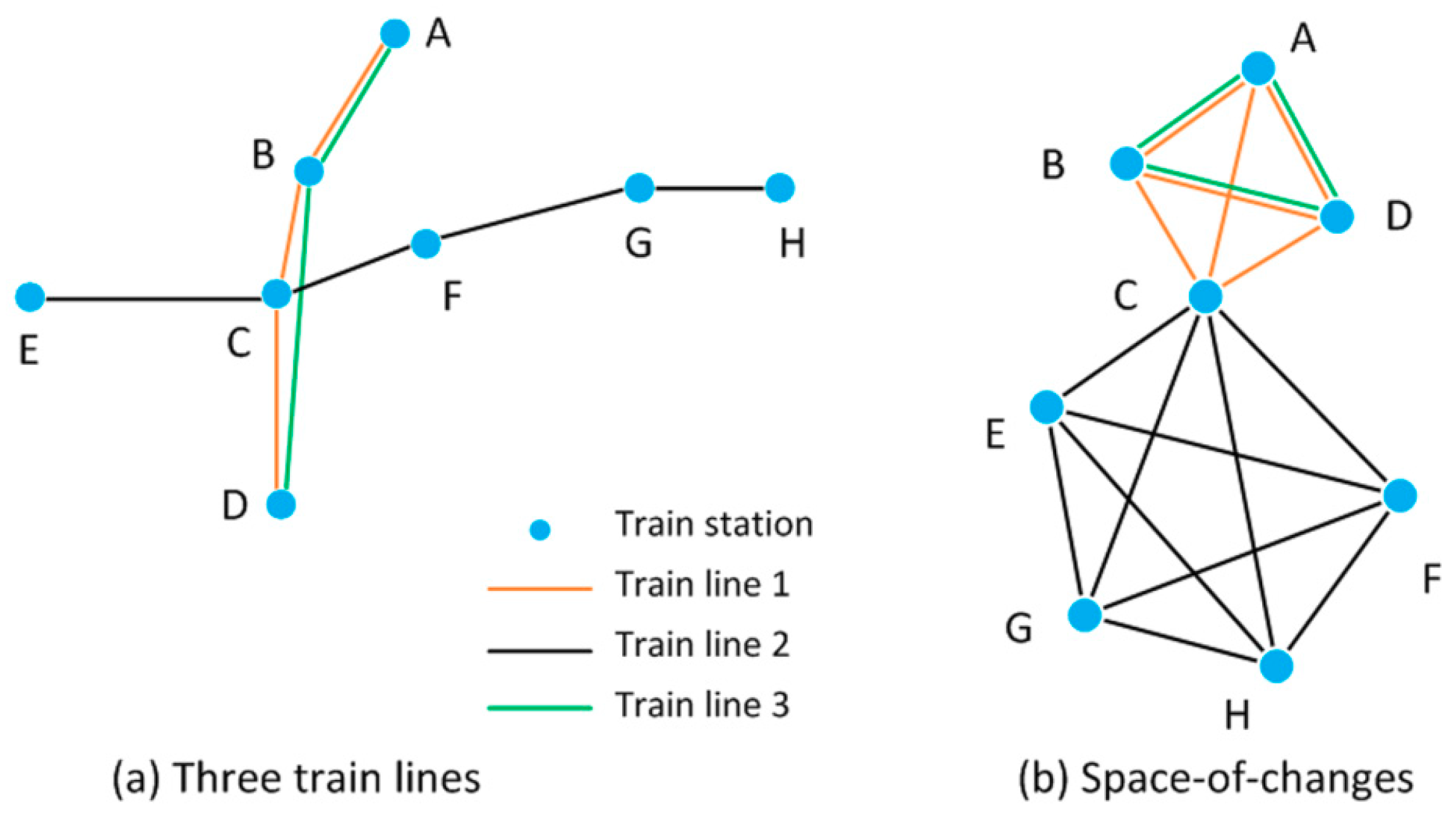
(2) For each directed pair of cities on the same train route, there is no need to make any transfer, as shown in Figure 3b. For instance, Train Line 3 passes through three cities of A-B-D. This line can be converted into three links: A-B, B-D and A-D. Under such rules, the weight matrix of a HSR network based on train timetables is A = {aij}
However, some cities had a different number of train stations at different points during the four stages covered by this study. Of the 2458 cities, 188 had no less than two train stations. For instance, Shanghai City has Shanghai Station, Shanghai South Station, Shanghai West Station, and Shanghai Hongqiao Station. There were 2700 train stations in this national railroad network during the period covered by this study. All stations in one city are treated as one node (that is, the city where they are located) [6]. The locations (latitude and longitude) of all train stations and cities were matched using Google Map geocoding API.
4.2. Network Indices
To explore the dynamics of China’s railway network, this paper applied the commonly used complex network indices [22,24,37,38,39].
4.2.1. Degree
Degree is measured by the number of edges connected by a node, which also describes the connectivity of that node. The average degree of all nodes is called the average degree of the network.
The degree–degree correlation is used to analyze the correlation between node degree and the average degree of each node’s neighbors. This is done to examine the connection preference among nodes. If nodes with large degrees first connect to other nodes with large degrees, the network is considered to be positive. Conversely, if nodes with large degrees first connect to other nodes with smaller degrees, the network is considered to be negative.
4.2.2. Weight and Strength
In a weighted network, the strength Si of node i is defined as the sum of the weights of all the edges of node i.
4.2.3. Graph Density
Network density (de) is used to describe the density of the interconnections between nodes in a network. This is defined as the ratio of the actual number of edges to the upper limit of the number of edges in the network. This indicator is often used to measure the density and evolution trends of networks in traffic analysis. The network density is calculated as follows:
Here, E is the actual number of edges, and N is the total number of nodes in the network. The network density varies from 0 to 1. When the network is fully connected, d(G) is 1. When there is no connection in the network, d(G) is 0. However, networks with a density of 1 basically do not exist. The maximum density that can be found in any real network is 0.5 [40].
4.2.4. Clustering Coefficient
A clustering coefficient is used to measure the degree of clustering of network nodes. Generally, the clustering coefficient of a node refers to the ratio of the actual number of edges of neighbors to the maximum number of possible edges between them.
A degree-clustering coefficient correlation is used to investigate the relationship between average clustering coefficients and the degrees of node. This is generally used to analyze the agglomeration and hierarchy of network structure.
4.2.5. Shortest Path Length
The average path length is also known as the characteristic path length. The distance between the two nodes i and j in the network is defined as the least number of edges that connects the two nodes. The average path length of the network is defined as the average distance between any pair of nodes.
4.2.6. Small World Network
Small world property is an important characteristic in complex network theory, which indicates that any two nodes in a network can be accessed by a few number of links. In general, a small world network is characterized by a high clustering coefficient and a small shortest path length [41,42,43]. It is demonstrated that all scale-free networks are believed to display small-world properties [22].
5. Results and Discussion
5.1. General Changes of Railway Network
A P-space graph was built for each of the four stages, based on train timetables. Therefore, the number of train lines directly affects the weight matrix of the directed weighted network. Firstly, the distribution of the different types of trains was analyzed. All the train lines obtained via web crawler were divided into seven types, as shown in Table 4. From Stage 1 to Stage 2 (after the opening of the high speed rail service), the number of the last four types of trains did not change obviously. Also, the number of D trains was reduced by approximately 76 trains. From Stage 2 to Stage 3, the number of high speed rail lines increased by 104. The number of D trains increased by about 113 during the same period. The number of express trains increased by about 88, while the number of general trains decreased by 96. During Stage 4, the number of high-speed rail trains and intercity high-speed rail trains increased by 1382 and 920, respectively. The number of D trains and express trains increased by 675 and 447, respectively.
After turning the timetables of the different stages into a P-space graph, the node degree, weights, network diameter, average path length, graph density and clustering coefficient of China’s railway network during each stage were calculated, as shown in Table 5.
In general, a small world network has a similar average shortest path and a larger clustering coefficient when compared with the random network of the same size [44]. In this paper, average shortest path and clustering coefficient of the random network with the same size are about 7.85 and 0.003, respectively. For China’s railway network, the average shortest paths all exceeded 9.5 during the previous three stages. Specifically, this network indicator during Stage 1 and Stage 2 was much closer to 10, but was only 8.03 in Stage 4. In addition, the network diameter in Stage 1 was 54, but this figure decreased to only 34 in Stage 4, which was also the largest topological distance between cities within this network. These node pairs mostly originated in the northeast and moved southwest. However after the opening of the HSR services, especially in Stage 4, cities in the northeast and southwest could be connected by fewer train lines, due to the new long-distance HSR lines. The number of stations in the northeast (including Liaoning, Jilin and Heilongjiang provinces) now exceeds 660. That figure accounts for approximately 24.50% of all of China’s railway stations. The destinations of trains starting from these three provinces are mostly Beijing and Tianjin, which are two of the most important terminal hubs connecting northeastern China. As a result, these three provinces have a large number of stations, but most of them only connect to the provincial capitals. This led to more transfers during the previous three stages if passengers needed to connect to long-distance stations in the southwest.
In addition, the clustering coefficient is another important measurement of small-world properties. Generally, a high clustering coefficient would indicate an efficient network in terms of travel mobility. In Stage 1, the average clustering coefficient was only 0.31. In fact, the clustering coefficients during all three of the previous stages were all below 0.35 (which was very close to the value of the US and a little higher than that of the worldwide railway network). During Stage 4, however, the clustering coefficient has increased to 0.40, which is 30% higher than in Stage 1 and much better than that of random network. The increase of clustering coefficient of China’s railway network indicates that a city’s neighbors are also likely to connect to each other. To find the clustering coefficient of each separate city, in Stage 1, cities with a clustering coefficient of below 0.1 accounted for 39.11% of all cities. In Stage 4, this ratio has declined to approximately 28.45%, and these are mainly very large or very small cities in China. For very large cities (such as provincial capital cities), the number of neighboring cities is large, and they are far from fully connected with each other. For very small cities, the number of neighboring cities is very small, and they are not connected with each other. In addition, 13.50% of cities in all stages had clustering coefficients equal to 1. It is also worth pointing out that the connections of these cities are all less than 6.
In general, we can see from Table 5 that, from Stage 1 to Stage 4, the average clustering coefficient increased from 0.31 to 0.40. The average shortest path length decreased from 9.96 to 8.03. The increase in the average clustering coefficient and the decrease in the average shortest path show that the small world characteristics of China’s railway network are more and more obvious. These characteristics are also found in the transport networks of the US, India and many European countries [41,45,46].
5.2. Degree and Degree Distribution
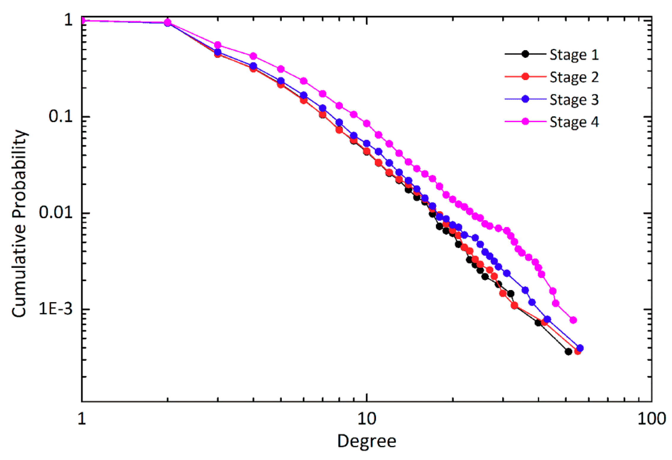
Figure 4 shows the cumulative probability distribution of node degree in each stage. In a logarithmic coordinate system, we can see that the node degree of China’s railway network during each stage obeyed the rule of power law distribution. This indicates that China’s railway network is an evolutionary, scale-free network. A few cities play a leading role in the railway network, while the development of other small and medium-sized cities is still restricted. Beijing, Shenyang, Wuhan, and Harbin are the most connected cities. Each of these cities’ degrees has exceeded 30 during all stages. However, the node degree is falling faster. In Stage 1, the highest degree was 51 (Beijing), while the tenth highest degree was only 22 (Xi’an). In Stage 4, the highest degree thus far is 53 (still Beijing), while the tenth highest degree is only 34 (now Nanjing). However, the average degree of each stage is well below these levels. The average degree of China’s railway network has been 3.43–4.22 at each stage. The ratio of cities below this average ranges from 66.78% to 68.82%. This indicates that the railway network shows strong heterogeneity in topology.
In addition, Figure 4 shows the cumulative probability of node degree distribution. Most nodes have a low degree; only a few nodes have a high degree. This indicates the distribution of node degree in each stage shows power law distribution (). The fitting results are shown in Table 6. The fitting accuracies measured by goodness of fit [47] are all close to 1. This finding further underlines the scaling free characteristics of China’s railway network. National hubs, such as Beijing, Wuhan, Zhengzhou, have very high degrees and play a leading role. However, the decrease of the power exponent indicates that the differences between node distributions have enlarged. Some regional stations not only play an important role in the national railway network, but also in connection with cities within other regions, such as Jinan.
As can be seen from Figure 4, the tail end of the blue line in Stage 4 is much higher than in the previous three stages. This indicates that operational policy changes (e.g., speed reductions, ticket fare reductions, and rearrangement of train timetables) have had little influence on the overall railway network degree distribution. In fact, these changes mainly affect those cities with large degrees. However, in Stage 4, the vigorous development of HSR and intercity HSR has had a significant impact on the overall railway network.
Domestic trains all use bidirectional train-routes. This means that, if there is a train running from Beijing to Shanghai, there will also be a train running from Shanghai to Beijing. In addition, their stop stations are all the same. Therefore, the in-degree, out-degree and degree of distribution will show identical distribution patterns. Thus, this study does not separately analyze in-degree and out-degree.
Table 7 shows the degree of the top 10 cities during all four stages. In total, 13 cities appear in the top 10 cities during the four stages. Beijing, Shenyang, and Wuhan have always had the highest degree during all four stages. Of the 13 cities, 12 are capital or municipal cities, located in the middle and eastern parts of China, as shown in Figure 5. This finding indicates that the regional hierarchy of the railway network is obvious. The greater the node degree, the more likely that node will be associated with more nodes, and the stronger the railway service capability will be.
5.3. Weight and Strength
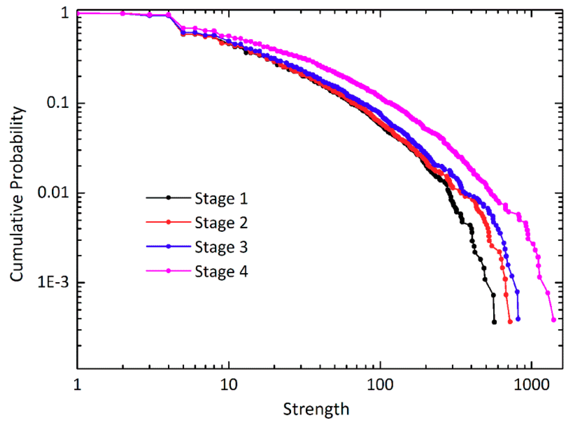
In most previous studies, passenger flow is used for determining the weight matrix. However, passenger flow data in small cities is difficult to obtain. Therefore, the effects of small cities in network analyses are frequently ignored. In this study, train lines in the national timetable are used for calculating the weight matrix. Thus, all cities served by the railway network can be taken into consideration in our network analysis. Figure 6 and Figure 7 show the distribution of weights and strengths in log-log coordinates.
In addition, the distribution curves of weight and strength during Stages 1–3 are very close to each other. However, in Stage 4, the curve is very different and most parts are above the curves of previous three stages. However, large cities are not dominant enough, and this leads to the scaling distribution being not rigorous. Significant changes and rearrangements of timetables have been introduced since the opening of HSR. The number of general and express trains has not increased, but the number of fast and direct express trains has increased by approximately 450 and 180, respectively. Most of the additional trains connect to cities without HSR services. Thus, the strength of these cities has increased as well. However, the number of HSR trains has dramatically increased, as shown in Table 4. New HSR lines have contributed to the dramatic increase in the strength of cities with HSR services. Thus, the strength of cities with HSR services has increased significantly. For example, the strength of Guiyang was 160 in Stage 3, when Guiyang was without a HSR service. However, the strength increased to 416 in Stage 4, after the introduction of a HSR service. The strength of Wuhan was 406 in Stage 1 (without HSR service), but increased to 1110 in Stage 4 (with HSR service).
Table 8 shows the strength of the top 10 cities during all four stages. As shown in Figure 8, the top 10 cities in terms of node strength are mainly distributed along the Beijing-Shanghai and Beijing-Wuhan-Guangzhou lines. The Beijing-Shanghai line is the main corridor connecting the north and east of China, while the Beijing-Wuhan-Guangzhou line is the most important corridor connecting the north and south of China. These two main corridors were also covered by HSR in previous stages. The frequency of HSR train routes on these two lines is also very high, which further reveals the “corridor effect” brought about by HSR. Of the 19 cities shown in Figure 8, 11 are provincial capital cities or municipalities, and six cities are close to two major hub cities, namely Shanghai and Guangzhou.
5.4. Degree–Degree Correlation
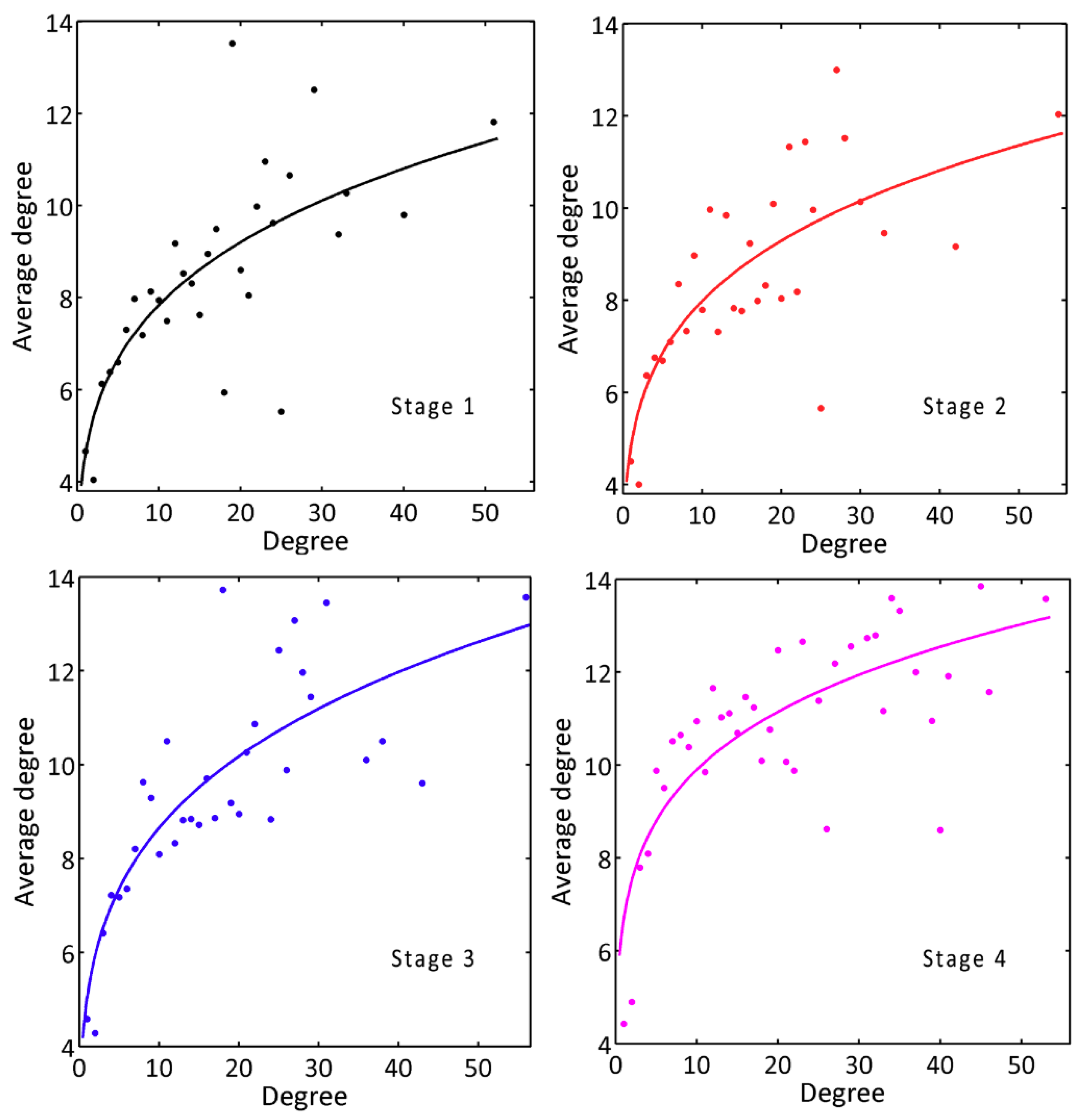
The degree–degree correlation indicates different connection preferences between nodes. Figure 9 shows the correlation between nodes degree and average degree of their neighbors. The average degree is much lower than the degree of that node. The Pearson correlation coefficient of each stage is 0.68, 0.67, 0.72 and 0.63, respectively. This indicates that a strong positive correlation exists between the degree and average degree of the neighbors. That is to say, the higher the degree of a node, the higher the average degree of their nearest neighbors. This pattern is totally different from the correlation result found in aviation networks and the Indian railway network [22,24]. However, the average degree fluctuates widely when node degree values are distributed between 10 and 30. Some cities are connected to those nodes with a higher degree to increase their connectivity. For example, the degree of Xiaogan city was only 5 in stage 1, but Xiaogan indirectly connected with Wuhan, whose degree is 33, thus improving Xiaogan’s connectivity. In the same way, some cities are connected to a lower degree of nodes to increase their connectivity, due to geographical constraints or urban functional requirements.
Moreover, the correlation can be roughly fitted with power law (). The fitting results are shown in Table 9. This pattern is very different from the results of previous aviation network research [24]. In an aviation network, the higher the degree of the nodes, the lower the average value of their neighbors [24]. The reason for this is that nodes with very small degree values are directly connected to cities with high degree values, in order to increase their accessibility in the network. However, unlike an aviation network, a railway network is more restricted by geographic constraints, and the cities with higher connectivity need to transfer through other cities. In China’s railway network, Beijing has the highest degree value, at more than 50 in all stages. The average degree value of Beijing’s neighboring nodes is also at a high level, with all above 11.
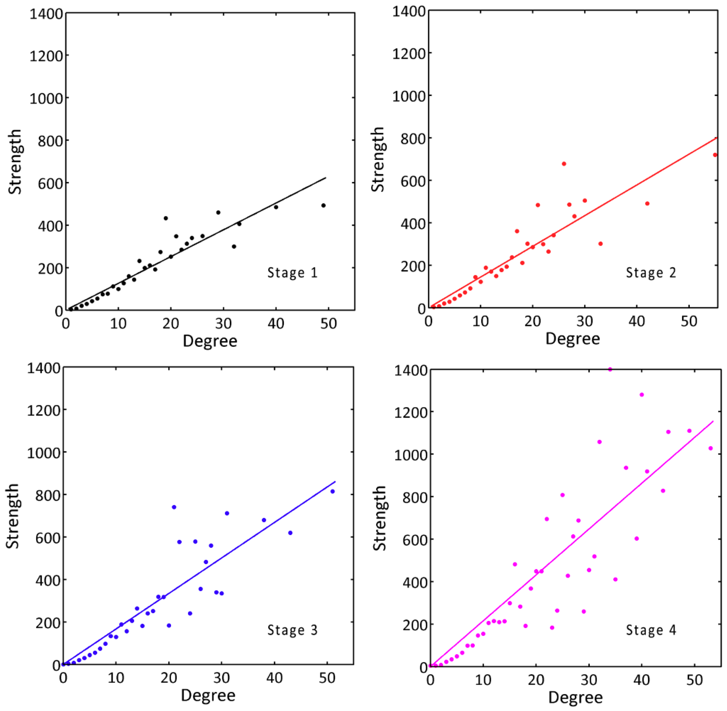
5.5. Degree-Strength Correlation
Figure 10 shows the correlation between node degree and average strength. The Pearson correlation coefficients of Stages 1–4 are 0.93, 0.90, 0.89 and 0.87, respectively. This indicates that a strong positive correlation exists between the strength and degree values of the nodes. The strength of nodes in HSR networks depends on the degree values of the nodes. As such, in the regression analysis, the constant variable is set as 0. Table 10 shows the fitting results of degree-strength correlation at all stages. The fitting accuracy of each stage is greater than 0.75. The slope of the fitting line increases from 12.60 in Stage 1, to 21.61 in Stage 4. This indicates that the introduction of HSR into a railway network can enhance the connections between nodes. This can be easily verified by the increase in the number of trains. For example, the strength of Wuhan was 406 in Stage 1. However, Wuhan’s strength has increased to over 1100 in Stage 4.
There is a positive linear correlation between degree and average strength. Therefore, in the next part, we simply verify the correlation between degree and clustering coefficient.
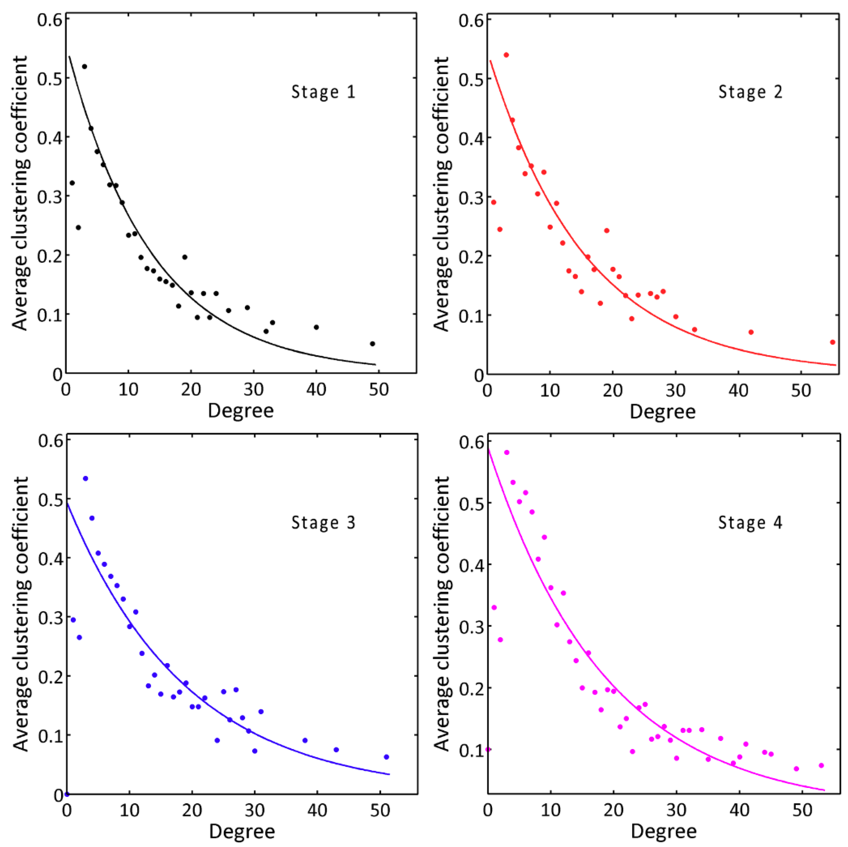
5.6. Degree-Clustering Coefficient Correlation
Figure 11 shows the correlation between node degree and average clustering coefficient with the same node degree. In general, there is no independence between the two indicators. The Pearson correlation coefficients of Stages 1–4 are −0.83, −0.80, −0.70, and −0.77, respectively. The higher the node degree is, the lower the clustering coefficient, which thus presents a negative correlation. This is consistent with existing conclusions presented in studies of aviation networks and the Indian railway network [22,24]. Neighbors of nodes with low degree levels are more easily clustered. However, nodes with higher degree or strength values are often built to be national hubs. These cities’ neighbors do not need to be directly connected, as can easily be connected through the transition between the high-degree cities. Thus, the clustering coefficient of these cities is lower (e.g., Beijing, Wuhan, Zhengzhou and Nanjing).
In addition, the correlation between node degree and the average clustering coefficient in each stage can be fitted using the decayed exponential law (). As shown in Table 11, the goodness of fit in each stage is more than 0.83. In view of the fitting coefficients, a is increasing, while power exponent b is decreasing from Stage 1 to Stage 4. This indicates that, with the development of China’s railway network, the decrease of the clustering coefficient slowed down only slightly. In Stage 4, the power exponent b is currently only −0.053. This is due to the fact that HSR can directly and effectively connect terminal cities with just a few stops, and regional nodes are more networked.
Generally speaking, the degree values of nodes with large clustering coefficients are small. In addition, some of these nodes are directly connected to national hubs, such as Beijing, Shanghai and Guangzhou, or regional hubs, like Nanjing, Xi’an and Chengdu. In a real railway network, there is no requirement for every node to be directly connected. They must simply be connected through nodes with higher centrality. The neighbors of low degree nodes are more inclined to be clustered than the neighbors of high degree nodes. The decrease of power law coefficient also indicates that the hierarchical network structure of China’s railway is more obvious.
6. Conclusions
This study first reviews the growth of China’s railway network over the past decade. Because of the introduction of high speed railway (HSR), China’s railway system has made rapid progress in terms of the increase in network mileage. The evolving characteristics of China’s railway network under the impact of HSR are studied here from a complex network perspective, including the topology indices of the network and the correlations between those indices. We found that, during the evolution of China’s railway network, the shortest path length reduced from 9.96 in Stage 1, to 8.03 in Stage 4. Also, the clustering coefficient increased from 0.31 in Stage 1, to 0.40 in Stage 4. The increase of clustering coefficient and decrease of shortest path length indicate that the small world characteristics of China’s railway network are more obvious. In addition, the distribution of node degree in each stage presents power law distribution. In the evolution of China’s railway network, the cities with higher degree values have been more stable. They have formed the skeleton and presented a hierarchical network structure over time, due to the leading roles played by the national-level hubs. However, the decrease of the fitting exponents indicates that the uneven distribution of degrees in China’s railway network is gradually enlarging. This is conducive to the formation of regional hub city sites, and these regional hub stations are conducive to the connection between urban nodes with lower degree values. This mechanism could illuminate policy makers to better construct regional HSR system to improve the connectivity of the whole railway network.
Moreover, this study reveals the hierarchical structure characteristics of China’s railway network through a correlation analysis between network indices. Our results indicate that a high correlation exists between degree and average degree, degree and strength, and degree and clustering coefficient. Nodes with higher degree values have higher strength. Also, the average degree of the nearest neighbors is higher, but the clustering coefficient shows a strong negative correlation with degree values. This could be characterized by exponential decay. In addition, the absolute value of exponential coefficients increased from 0.053 in Stage 1, to 0.074 in Stage 4. This indicates that adjacent nodes tend to be networked to a greater degree, and the hierarchical network structure of China’s railway is more obvious.
This research is of great significance in terms of gaining a better understanding of the evolution of China’s railway network and how that network has been affected by operational policies, construction plans and operating mechanisms. Thus, our work can be referenced by railway companies and the relevant departments when planning the future of HSR and optimizing China’s rail network. For instance, the analysis of changes of policy decisions in different stages can be useful for policy makers to gain insights of potential impacts on network efficiency due to proposed changes of operating speed, or timetables of railroad operations.
Finally, this research is an exploratory study, however, we do note several limitations, such as:
(1) Few transport network studies have paid attention to the spatial autocorrelation [22,23,24], however, the evolution of transport network may be spatially related. Thus, spatial autocorrelation should be taken into consideration in transport network analysis.
(2) The dataset acquired from the website lacks the detailed information of passenger flows. The passenger flow data may be more appropriate and objective for weighting the connectivity between each city pair in transport network analysis.
(3) The evolution of railway network are highly sensitive to political, economic, demographic and geographical factors. Thus, more socio-economic factors could be considered when modeling the development of railway systems.
Author Contributions
The research was mainly conceived and designed by Y.H. and S.L. S.L., X.Y. and Z.Z. performed the experiments and wrote the manuscript. Y.H. and S.L. reviewed the manuscript and provided comments.
Funding
This research was jointly supported by National Natural Science Foundation of China (Grants 51478199 and 51538004), and China Postdoctoral Science Foundation (Nos. 2018M632860, 2017M623112), and the Foundation of Geomatics Technology and Application key Laboratory of Qinghai Province (No. QHDX-2018-08).
Acknowledgments
The authors would like to thank the valuable comments from anonymous reviewers.
Conflicts of Interest
The authors declare no conflict of interest.
References
- Wang, J.; Jin, F.; Mo, H.; Wang, F. Spatiotemporal evolution of China’s railway network in the 20th century: An accessibility approach. Transp. Res. Part A Policy Pract. 2009, 43, 765–778. [Google Scholar] [CrossRef]
- Wandelt, S.; Wang, Z.; Sun, X. Worldwide railway skeleton network: Extraction methodology and preliminary analysis. IEEE Trans. Intell. Transp. Syst. 2017, 18, 2206–2216. [Google Scholar] [CrossRef]
- National Bureau of Statistics of China. International Statistical Yearbook 2016. Available online: http://data.s tats.gov.cn/files/lastestpub/gjnj/2016/indexch.htm (accessed on 3 May 2018).
- National Bureau of Statistics of China. China Statistical Yearbook 2017. Available online: http://www.stats.gov.c n/tjsj/ndsj/2017/indexch.htm (accessed on 3 May 2018).
- Cao, J.; Liu, X.C.; Wang, Y.; Li, Q. Accessibility impacts of China’s high-speed rail network. J. Transp. Geogr. 2013, 28, 12–21. [Google Scholar] [CrossRef]
- Shaw, S.-L.; Fang, Z.; Lu, S.; Tao, R. Impacts of high speed rail on railroad network accessibility in China. J. Transp. Geogr. 2014, 40, 112–122. [Google Scholar] [CrossRef]
- Wu, W.; Liang, Y.; Wu, D. Evaluating the Impact of China’s Rail Network Expansions on Local Accessibility: A Market Potential Approach. Sustainability 2016, 8, 512. [Google Scholar] [CrossRef]
- Sánchez-Mateos, H.S.M.; Givoni, M. The accessibility impact of a new High-Speed Rail line in the UK—A preliminary analysis of winners and losers. J. Transp. Geogr. 2012, 25, 105–114. [Google Scholar] [CrossRef]
- Shi, J.; Zhou, N. How cities influenced by high speed rail development: A case study in China. J. Transp. Technol. 2013, 3, 7–16. [Google Scholar] [CrossRef]
- Jiao, J.; Wang, J.; Jin, F.; Dunford, M. Impacts on accessibility of China’s present and future HSR network. J. Transp. Geogr. 2014, 40, 123–132. [Google Scholar] [CrossRef]
- Kim, H.; Sultana, S. The impacts of high-speed rail extensions on accessibility and spatial equity changes in South Korea from 2004 to 2018. J. Transp. Geogr. 2015, 45, 48–61. [Google Scholar] [CrossRef]
- Chester, M.V.; Ryerson, M.S. Grand challenges for high-speed rail environmental assessment in the United States. Transp. Res. Part A 2014, 61, 15–26. [Google Scholar] [CrossRef]
- Chen, Z.; Xue, J.; Rose, A.Z.; Haynes, K.E. The impact of high-speed rail investment on economic and environmental change in China: A dynamic CGE analysis. Transp. Res. Part A Policy Pract. 2016, 92, 232–245. [Google Scholar] [CrossRef]
- Cheng, Y.S.; Loo, B.P.Y.; Vickerman, R. High-speed rail networks, economic integration and regional specialisation in China and Europe. Travel Behav. Soc. 2015, 2, 1–14. [Google Scholar] [CrossRef] [Green Version]
- Yang, Y.; Liu, Y. Urban spatial structure influenced by the introduction of high-speed railway terminal. In Proceedings of the International Conference on Remote Sensing, Environment and Transportation Engineering, Nanjing, China, 24–26 June 2011; IEEE: Piscataway, NJ, USA, 2011; pp. 5621–5624. [Google Scholar]
- Shen, Y.; Silva, J.D.; Martínez, L.M. Assessing High-Speed Rail’s impacts on land cover change in large urban areas based on spatial mixed logit methods: A case study of Madrid Atocha railway station from 1990 to 2006. J. Transp. Geogr. 2014, 41, 184–196. [Google Scholar] [CrossRef]
- Guimerà, R.; Mossa, S.; Turtschi, A.; Amaral, L.N. The worldwide air transportation network: Anomalous centrality, community structure, and cities’ global roles. Proc. Natl. Acad. Sci. USA 2005, 102, 7794–7799. [Google Scholar] [CrossRef] [PubMed]
- Gallos, L.K.; Song, C.; Havlin, S.; Makse, H.A. Scaling theory of transport in complex biological networks. Proc. Natl. Acad. Sci. USA 2007, 104, 7746–7751. [Google Scholar] [CrossRef] [PubMed] [Green Version]
- Ľuboš, B.; Rui, C. Controlling congestion on complex networks: Fairness, efficiency and network structure. Sci. Rep. 2017, 7, 9152. [Google Scholar]
- Newman, M.E. Modularity and community structure in networks. Proc. Natl. Acad. Sci. USA 2006, 103, 8577–8582. [Google Scholar] [CrossRef] [PubMed] [Green Version]
- Newman, M.E. Networks: An Introduction; Oxford University Press, Inc.: Oxford, UK, 2010. [Google Scholar]
- Sen, P.; Dasgupta, S.; Chatterjee, A.; Sreeram, P.A.; Mukherjee, G.; Manna, S.S. Small-world properties of the Indian railway network. Phys. Rev. E Stat. Nonlinear Soft Matter Phys. 2003, 67, 036106. [Google Scholar] [CrossRef] [PubMed] [Green Version]
- Li, W.; Cai, X. Empirical analysis of a scale-free railway network in China. Phys. A Stat. Mech. Appl. 2007, 382, 693–703. [Google Scholar] [CrossRef]
- Lin, J. Network analysis of China’s aviation system, statistical and spatial structure. J. Transp. Geogr. 2012, 22, 109–117. [Google Scholar] [CrossRef]
- Verma, T.; Araújo, N.A.M.; Herrmann, H.J. Revealing the structure of the world airline network. Sci. Rep. 2014, 4, 5638. [Google Scholar] [CrossRef] [PubMed]
- Kaluza, P.; Kölzsch, A.; Gastner, M.T.; Blasius, B. The complex network of global cargo ship movements. J. R. Soc. Interface 2010, 7, 1093. [Google Scholar] [CrossRef] [PubMed]
- Zaidi, F. Maritime constellations: A complex network approach to shipping and ports. Marit. Policy Manag. 2012, 39, 151–168. [Google Scholar]
- Zhang, J.; Wang, S.; Wang, X. Comparison analysis on vulnerability of metro networks based on complex network. Phys. A Stat. Mech. Appl. 2018, 496, 72–78. [Google Scholar] [CrossRef]
- Brockmann, D.; Hufnagel, L.; Geisel, T. The scaling laws of human travel. Nature 2006, 439, 462–465. [Google Scholar] [CrossRef] [PubMed] [Green Version]
- Liang, X.; Zhao, J.; Li, D.; Ke, X. Unraveling the origin of exponential law in intra-urban human mobility. Sci. Rep. 2013, 3, 65. [Google Scholar] [CrossRef] [PubMed]
- Dodds, P.S.; Muhamad, R.; Watts, D.J. An experimental study of search in global social networks. Science 2003, 301, 827–829. [Google Scholar] [CrossRef] [PubMed]
- Szell, M.; Lambiotte, R.; Thurner, S. Multirelational organization of large-scale social networks in an online world. Proc. Natl. Acad. Sci. USA 2010, 107, 13636–13641. [Google Scholar] [CrossRef] [PubMed] [Green Version]
- Ghosh, S.; Banerjee, A.; Sharma, N.; Agarwal, S.; Ganguly, N.; Bhattacharya, S.; Mukherjee, A. Statistical analysis of the Indian Railway Network: A complex network approach. Acta Phys. Pol. B Proc. Suppl. 2011, 4, 123–138. [Google Scholar] [CrossRef]
- Sun, Y.; Cao, C.; Wu, C. Multi-objective optimization of train routing problem combined with train scheduling on a high-speed railway network. Transp. Res. Part C 2014, 44, 1–20. [Google Scholar] [CrossRef]
- Sienkiewicz, J.; Hołyst, J.A. Statistical analysis of 22 public transport networks in Poland. Phys. Rev. E Stat. Nonlinear Soft Matter Phys. 2005, 72, 046127. [Google Scholar] [CrossRef] [PubMed]
- Kurant, M.; Thiran, P. Extraction and analysis of traffic and topologies of transportation networks. Phys. Rev. E Stat. Nonlinear Soft Matter Phys. 2006, 74, 036114. [Google Scholar] [CrossRef] [PubMed]
- Hossain, M.M.; Alam, S. A complex network approach towards modeling and analysis of the Australian Airport Network. J. Air Transp. Manag. 2017, 60, 1–9. [Google Scholar] [CrossRef]
- Dai, L.; Derudder, B.; Liu, X. The evolving structure of the Southeast Asian air transport network through the lens of complex networks, 1979–2012. J. Transp. Geogr. 2018, 68, 67–77. [Google Scholar] [CrossRef] [Green Version]
- Xu, W.; Zhou, J.; Qiu, G. China’s high-speed rail network construction and planning over time: A network analysis. J. Transp. Geogr. 2018, 70, 40–54. [Google Scholar] [CrossRef]
- Mayhew, B.H.; Levinger, R.L. Size and the Density of Interaction in Human Aggregates. Am. J. Sociol. 1976, 82, 86–110. [Google Scholar] [CrossRef]
- Du, W.B.; Zhou, X.L.; Lordan, O.; Wang, Z.; Zhao, C.; Zhu, Y.B. Analysis of the Chinese Airline Network as multi-layer networks. Transp. Res. Part E 2016, 89, 108–116. [Google Scholar] [CrossRef]
- Chopra, S.; Dillon, T.; Bilec, M.; Khanna, V. A network-based framework for assessing infrastructure resilience: A case study of the London metro system. J. R. Soc. Interface 2016, 13, 20160113. [Google Scholar] [CrossRef] [PubMed]
- Chatterjee, A.; Manohar, M.; Ramadurai, G. Statistical Analysis of Bus Networks in India. PLoS ONE 2016, 11, e0168478. [Google Scholar] [CrossRef] [PubMed]
- Wang, J.; Mo, H.; Wang, F.; Jin, F. Exploring the network structure and nodal centrality of China’s air transport network: A complex network approach. J. Transp. Geogr. 2011, 19, 712–721. [Google Scholar] [CrossRef]
- Bagler, G. Analysis of the airport network of India as a complex weighted network. Phys. A Stat. Mech. Appl. 2008, 387, 2972–2980. [Google Scholar] [CrossRef] [Green Version]
- Wandelt, S.; Sun, X.; Zhang, J. Evolution of domestic airport networks: A review and comparative analysis. Transportmetrica B 2017, 13, 1–17. [Google Scholar] [CrossRef]
- Leung, Y.; Mei, C.L.; Zhang, W.X. Statistical tests for spatial nonstationarity based on the geographically weighted regression model. Environ. Plan. A 2000, 32, 9–32. [Google Scholar] [CrossRef]
Figure 1.
Mileage of China’s railway service.

Figure 2.
Spatial distribution of rail lines during different stages.

Figure 3.
P-space graph of railway lines.

Figure 4.
Cumulative probability of degree distribution in different stages.

Figure 5.
Spatial distribution of the degree of top 10 cities.
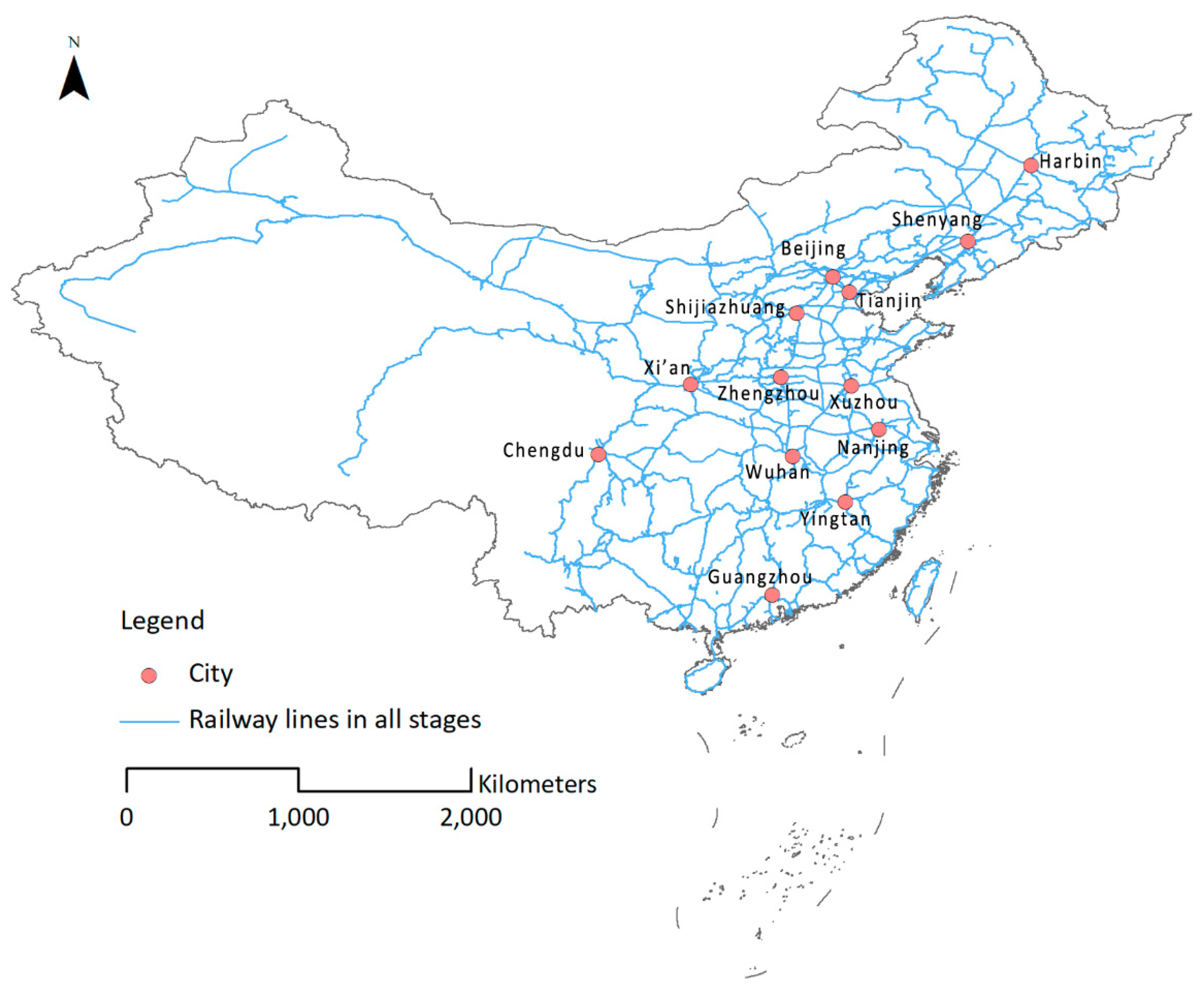
Figure 6.
Cumulative probability of weight distribution.
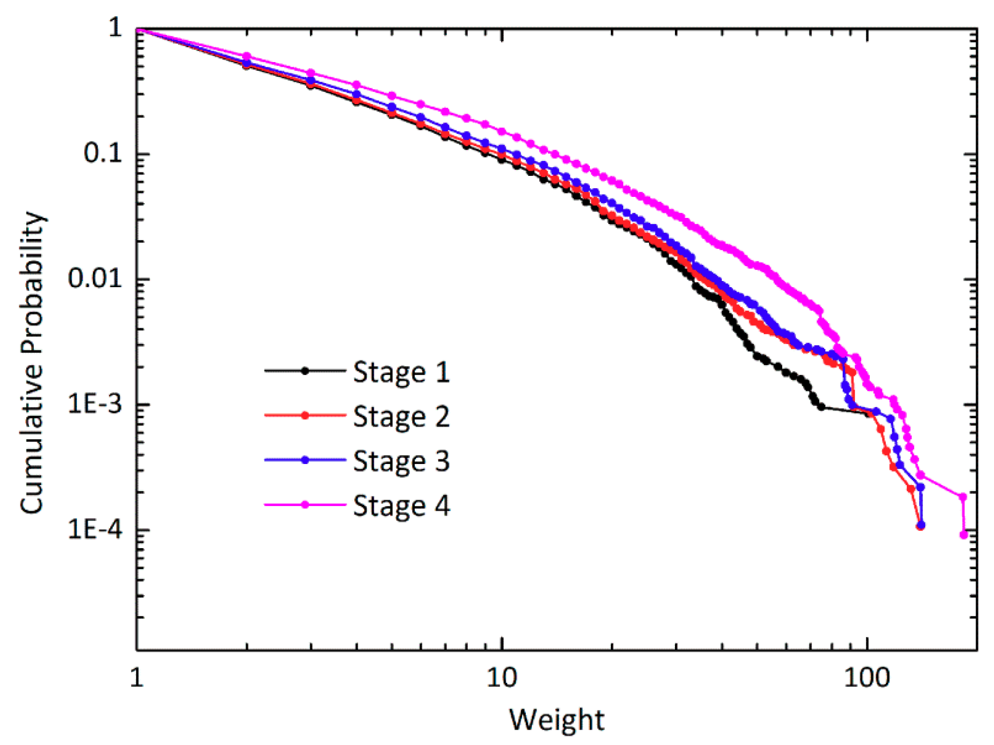
Figure 7.
Cumulative probability of strength distribution.

Figure 8.
Spatial distribution of the weights of top 10 cities.

Figure 9.
Degree–degree correlation.

Figure 10.
Degree-strength correlation.

Figure 11.
Degree-clustering coefficient correlation.


Table 1.
Four stages of China’s railway development from 2008–2017.
| Stage | Time Period | HSR Lines |
|---|---|---|
| 1 | Before August 2008 | Conventional railway network, no HSR service |
| 2 | Between August 2008 and July 2011 | Preliminary construction |
| 3 | Between July 2011 and January 2013 | Network skeleton: Several new HSR lines were built |
| 4 | Between January 2013 and July 2017 | Deep intensification |
Table 2.
Seven types of passenger train service.
| Train Service Type | G | D | C | Z | T | K | P |
|---|---|---|---|---|---|---|---|
| Description | HSR Train | HSR Train | Intercity-HSR | Direct Exp. Train | Express Train | Fast Train | General Train |
| Max speed (km/h) | [300, 350] | [250, 300] | [200, 250] | 160 | 140 | 120 | 100 |
Table 3.
Timetable of train route G107 in the Stage 2.
| Station | Arrival Time | Departure Time | Stop Time (min.) | Distance from the Origin Station (km) | Ticket Fare (yuan) |
|---|---|---|---|---|---|
| 1. Beijing South | - | 08:15 | - | - | - |
| 2. Dezhou East | 09:28 | 09:30 | 2 | 314 | 145 |
| 3. Jinan West | 09:54 | 09:56 | 2 | 424 | 185 |
| 4. Tai’an | 10:13 | 10:14 | 1 | 486 | 214 |
| 5. Qufu East | 10:34 | 10:35 | 1 | 577 | 244 |
| 6. Nanjing South | 12:20 | 12:27 | 7 | 1023 | 444 |
| 7. Danyang North | 12:52 | 12:53 | 1 | 1120 | 479 |
| 8. Shanghai Hongqiao | 13:40 | - | - | 1318 | 553 |
Table 4.
Seven types of passenger train service.
| Train Service Type | G | D | C | Z | T | K | P | |
|---|---|---|---|---|---|---|---|---|
| Amount | Stage 1 | 0 | 1002 | 0 | 54 | 253 | 1121 | 843 |
| Stage 2 | 459 | 926 | 162 | 52 | 260 | 1136 | 830 | |
| Stage 3 | 663 | 1039 | 167 | 52 | 275 | 1224 | 734 | |
| Stage 4 | 2045 | 1714 | 1087 | 237 | 226 | 1671 | 508 | |
Table 5.
The whole railway network index in four stages.
| Index | Stage 1 | Stage 2 | Stage 3 | Stage 4 |
|---|---|---|---|---|
| Average Degree (k) | 3.43 | 3.45 | 3.59 | 4.22 |
| Average Strength (S) | 13.16 | 14.16 | 16.00 | 24.13 |
| Graph Diameter (d) | 54 | 53 | 50 | 34 |
| Average Shortest Path (l) | 9.96 | 9.97 | 9.50 | 8.03 |
| Graph Density | 0.001 | 0.001 | 0.001 | 0.002 |
| Average Clustering Coefficient (C) | 0.31 | 0.32 | 0.34 | 0.40 |
Table 6.
Power law distribution of degree.
| Power Law | Stage 1 | Stage 2 | Stage 3 | Stage 4 |
|---|---|---|---|---|
| a | 3.27 | 3.29 | 3.01 | 2.71 |
| b | −1.77 | −1.78 | −1.67 | −1.45 |
| R2 | 0.99 | 0.99 | 0.99 | 0.99 |
Table 7.
Degree for the top 10 cities in four stages.
| Top 10 | Stage 1 | Stage 2 | Stage 3 | Stage 4 | ||||
|---|---|---|---|---|---|---|---|---|
| Degree | City | Degree | City | Degree | City | Degree | City | |
| 1st | 51 | Beijing | 55 | Beijing | 56 | Beijing | 53 | Beijing |
| 2nd | 40 | Shenyang | 42 | Shenyang | 43 | Shenyang | 51 | Wuhan |
| 3rd | 33 | Wuhan | 33 | Harbin | 38 | Wuhan | 46 | Shenyang |
| 4th | 32 | Harbin | 30 | Wuhan | 36 | Harbin | 45 | Zhengzhou |
| 5th | 29 | Zhengzhou | 28 | Nanjing | 31 | Nanjing | 41 | Guangzhou |
| 6th | 26 | Xuzhou | 28 | Xuzhou | 31 | Zhengzhou | 41 | Tianjin |
| 7th | 25 | Chengdu | 27 | Zhengzhou | 28 | Shijiazhuang | 39 | Xi’an |
| 8th | 23 | Shijiazhuang | 25 | Chengdu | 27 | Xi’an | 39 | Chengdu |
| 9th | 22 | Yingtan | 23 | Xi’an | 26 | Yingtan | 37 | Xuzhou |
| 10th | 22 | Xi’an | 23 | Yingtan | 26 | Xuzhou | 34 | Nanjing |
Table 8.
Strength for the top 10 cities in four stages.
| Top 10 | Stage 1 | Stage 2 | Stage 3 | Stage 4 | ||||
|---|---|---|---|---|---|---|---|---|
| Strength | City | Strength | City | Strength | City | Strength | City | |
| 1st | 568 | Dongguan | 720 | Beijing | 816 | Beijing | 1400 | Nanjing |
| 2nd | 558 | Guangzhou | 678 | Nanjing | 804 | Nanjing | 1280 | Guangzhou |
| 3rd | 492 | Beijing | 668 | Shanghai | 740 | Guangzhou | 1128 | Hangzhou |
| 4th | 486 | Shenyang | 642 | Guangzhou | 698 | Shanghai | 1110 | Wuhan |
| 5th | 460 | Zhengzhou | 632 | Suzhou | 680 | Wuhan | 1104 | Zhengzhou |
| 6th | 422 | Hangzhou | 612 | Wuxi | 668 | Suzhou | 1058 | Changsha |
| 7th | 418 | Shijiazhuang | 548 | Changzhou | 656 | Wuxi | 1028 | Beijing |
| 8th | 406 | Wuhan | 526 | Zhuzhou | 620 | Shenyang | 948 | Shanghai |
| 9th | 404 | Shilong | 524 | Dongguan | 620 | Zhengzhou | 946 | Suzhou |
| 10th | 404 | Zhangmutou | 522 | Changsha | 602 | Tianjin | 936 | Xuzhou |
Table 9.
Correlation results of degree–degree correlation.
| Power Law | Stage 1 | Stage 2 | Stage 3 | Stage 4 |
|---|---|---|---|---|
| a | 4.60 | 4.82 | 5.04 | 6.68 |
| b | 0.23 | 0.22 | 0.23 | 0.17 |
| R2 | 0.54 | 0.56 | 0.67 | 0.58 |
Table 10.
Correlation results of degree-degree.
| Linear | Stage 1 | Stage 2 | Stage 3 | Stage 4 |
|---|---|---|---|---|
| a | 12.60 | 14.45 | 16.71 | 21.61 |
| R2 | 0.86 | 0.80 | 0.79 | 0.75 |
Table 11.
Correlation results of degree-clustering coefficient.
| Exponential Law | Stage 1 | Stage 2 | Stage 3 | Stage 4 |
|---|---|---|---|---|
| a | 0.56 | 0.55 | 0.49 | 0.59 |
| b | −0.074 | −0.064 | −0.052 | −0.053 |
| R2 | 0.93 | 0.89 | 0.83 | 0.85 |
© 2018 by the authors. Licensee MDPI, Basel, Switzerland. This article is an open access article distributed under the terms and conditions of the Creative Commons Attribution (CC BY) license (http://creativecommons.org/licenses/by/4.0/).
Share and Cite
MDPI and ACS Style
Huang, Y.; Lu, S.; Yang, X.; Zhao, Z. Exploring Railway Network Dynamics in China from 2008 to 2017. ISPRS Int. J. Geo-Inf. 2018, 7, 320. https://doi.org/10.3390/ijgi7080320
AMA Style
Huang Y, Lu S, Yang X, Zhao Z. Exploring Railway Network Dynamics in China from 2008 to 2017. ISPRS International Journal of Geo-Information. 2018; 7(8):320. https://doi.org/10.3390/ijgi7080320
Chicago/Turabian StyleHuang, Yaping, Shiwei Lu, Xiping Yang, and Zhiyuan Zhao. 2018. "Exploring Railway Network Dynamics in China from 2008 to 2017" ISPRS International Journal of Geo-Information 7, no. 8: 320. https://doi.org/10.3390/ijgi7080320
Note that from the first issue of 2016, this journal uses article numbers instead of page numbers. See further details here.