Multidimensional Arrays for Analysing Geoscientific Data


1
Institute for Geoinformatics, University of Muenster, 48149 Muenster, Germany
2
Department of Physical Geography, Faculty of Geoscience, Utrecht University, 3584 CB Utrecht, The Netherlands
*
Author to whom correspondence should be addressed.
†
Current address: Vening Meinesz Building A, Princetonlaan 8A, 3584 CB Utrecht, The Netherlands.
ISPRS Int. J. Geo-Inf. 2018, 7(8), 313; https://doi.org/10.3390/ijgi7080313
Submission received: 27 June 2018
/
Revised: 20 July 2018
/
Accepted: 30 July 2018
/
Published: 3 August 2018
Abstract
:Geographic data is growing in size and variety, which calls for big data management tools and analysis methods. To efficiently integrate information from high dimensional data, this paper explicitly proposes array-based modeling. A large portion of Earth observations and model simulations are naturally arrays once digitalized. This paper discusses the challenges in using arrays such as the discretization of continuous spatiotemporal phenomena, irregular dimensions, regridding, high-dimensional data analysis, and large-scale data management. We define categories and applications of typical array operations, compare their implementation in open-source software, and demonstrate dimension reduction and array regridding in study cases using Landsat and MODIS imagery. It turns out that arrays are a convenient data structure for representing and analysing many spatiotemporal phenomena. Although the array model simplifies data organization, array properties like the meaning of grid cell values are rarely being made explicit in practice.
1. Introduction
An array is a storage form for a sequence of objects of similar type. In principle, data tables, collections of records of identical type, are one-dimensional arrays when the records form a sequence. Time series data, such as daily mean temperatures for a measurement site, form a natural one-dimensional array with the time stamp unambiguously ordering the observations, but more typically arrays will have rows and columns, creating two-dimensional arrays, or be higher dimensional.
For geoscientific data, arrays typically arise when we try to represent a phenomenon that varies continuously over space and time, or a field variable [1,2], by regularly discretising space and time. Data on such phenomena can be the result of observation or computation. Examples of observed arrays are remote sensing imagery or digital photography: image pixels represent reflectance of a certain colour averaged over a spatial region and a short time period, the exposure time. The observed area depends on the image sensor density, the focal distance of the lens, and the distance to the observed object. As an example of a computed array, weather or climate models typically solve partial differential equations by dividing the Earth into areas, which could be arrays with regular longitude and latitude (e.g., a 0.1× 0.1 grid). Two-dimensional arrays can partition a two-dimensional surface in square cells with constant size, but representing a spherical (or ellipsoidal) surface, such as the Earth’s surface, by a two-dimensional array leads to grid cells that are no longer squares or have constant area [3]. Elevation, or depth, is often discretised in irregular steps.
In addition to challenges that arise from irregularities in grid cell sizes, or irregularly chosen grid distances [4], typical questions to geoscientific array data relate to what the array grid cell value exactly refers to: does it represent the point value at the location of the grid cell centre, does it represent a constant value throughout the whole grid cell (i.e., at all point locations within the grid), does it represent an aggregation of the variable over the grid region, or something else [2]? In spatial statistics, the physical area (or volume, or duration) an observation or predictions is associated with is called support of the data [5]. The different possibilities may not matter much when combining arrays with identical properties, but do play a role when comparing them to other arrays, converting (regridding) one to the cells of another, or combining them with other, non-array data such as features (points, lines, polygons) in a GIS [6].
Natural phenomena are commonly high dimensional and are represented into arrays when digitalized. The high dimensionality of data makes them challenging to be analyzed and processed. Dimension reduction methods are array methods aiming at finding a suitable representation of high dimensional data to extract useful information. A classical orthogonal covariance/correlation-based transformation method is PCA (Principle Component Analysis), which has various extensions. For example, ICA (Independent Component Analysis, [7]) is a higher order entrophy-based transformation that further minimizes variable independence. MNF (Maximum Noise Fraction, [8]) is specifically designed to remove noise from spatiotemporal data and apply to space-time ordered matrices.
To efficiently access and analyze array data, array storage have been extensively discussed [9], and a variety of array algebra and software systems have been developed [10,11,12]. A comprehensive survey of array query languages, chunking strategies, and array database systems untill 2013 could be found in [13]. Ref. [14] attempted to create a general benchmark (known as SS-DB) to quantitatively evaluate performances of array database systems, and [15] further formalised the representation of SS-DB. Our study distinguishes from surveying array data processing techniques [13] and establishing benchmarks [15] and focuses on challenges from geoscientific arrays. We review array abstraction of space-time phenomena, geographic data analysis methods on arrays and several array data analytic and management systems in terms of their features in supporting geographical analysis and the array operations that are implemented.
A variety of mathematical methods, algebra and software of arrays have been developed; however, the progresses and challenges of using arrays to model geosicentific data have not been thoroughly reviewed and discussed before. Our objective is to review the generic information storage model of multidimensional arrays in the context of representing and analyzing geoscientific data. In addition, we provide two small study cases applying regridding and dimension reduction, to make their link with the array model more concrete, and to illustrate how array methods are implemented in array model and to point out the different outcomes resulting from different software implementations for identical methods.
The manuscript is structured as follows: We give an overview of arrays (Section 2) and manipulation operations (Section 3). We compare different open source software implementations suitable more and less dedicated to geoscientific data, and show that for similar operations the syntax and function names used varies strongly (Section 4). We then focus on commonly recurring challenges: regridding and dimension reduction (Section 5). We provide two small study cases applying regridding and dimension reduction. The regridding study case shows how different array regridding methods and implementations in different software affect results. The dimension reduction study case shows how array operations and software are used to provide a clean and scalable data analysis process (Section 6). In discussion (Section 7), we further discuss array abstraction of continuous spatiotemporal phenomenon, the current challenges of sparse array, array software and regridding in handling geoscientific data, multidimensional statistical methods such as joint spatiotemporal analysis and dimension reduction on arrays, and finish with a conclusion.
2. What Are Multidimensional Arrays?
Arrays are fundamental data structures in computer science that store collections of equally typed variables. Array elements can be accessed by indexes that are directly translated to memory addresses. In contrast to linked lists, arrays support random access in constant time. Array indexes are usually integers though many programming languages implement associative arrays with arbitrary index data type. Arrays can be indexed by multiple dimensions that map to a one-dimensional array in order to fit linear computer memory.
Besides their use in programming languages, arrays can be extended to a flexible data structure for data-oriented sciences [16]. A multidimensional array then can be seen as a function that maps the Cartesian product of multiple discrete, totally ordered, and finite dimensions to a multidimensional attribute space. Let D denote an n-dimensional index or dimension space and V refer to an m-dimensional attribute or value space. An array A is then defined as , where , , and individual dimensions are finite and totally ordered. Implementations of the array model typically represent dimension values as integers. Due to the finiteness property, however, there always exists an invertible dimension transformation function that relates the array index integer number to the original dimension value.
Individual array dimensions may or may not have a natural physical interpretation such as space, time, or wavelength. Examples for rather artificial dimensions are station identifiers or record numbers that can be ordered as numbers or names with regard to their letters but do not have a natural order in the physical world.
For the remainder of this paper, we make the following definitions. A cell or pixel is a coordinate/point in the index/dimension space whereas a cell value denotes attribute values at that particular cell . We denote the number of elements of the i-th dimension as and the total number of cells as . The array schema defines dimensions and attribute types. If a dimension has a natural physical interpretation, cells have a well-defined size with regard to the dimension.
2.1. Types of Arrays
The above definition of multidimensional arrays is most generic. In the following, we distinguish between sparse vs. dense arrays and regular vs. irregular dimensions. An array is said to be sparse if the index space is a strict subset of the Cartesian product of individual dimensions. In practice, sparsity assumes that whereas arrays with only a few empty cells may be considered as dense and letting empty cells point to a dedicated undefined value that is added to the attribute space. Implementations for sparse arrays may reduce memory consumption and computation times in array-based analysis (see Section 4 or common sparse linear algebra routines).
A dimension is denoted regular if all pairs of successive elements (cells) have the same distance in that dimension. Let the j-th element of the (ordered) dimension . Then a dimension is regular if
where is then referred to as the cell size or sampling interval of dimension i. This distinction only applies to dimensions with meaningful distance measures. The advantage of regular dimensions is that the transformation of true dimension values to integer indexes can be computed directly from cell size and an offset value by an affine transformation, which does not require searching in the dimension space.
Other important types of arrays are vectors and matrices. Both have a single numeric attribute and artificial regular dimensions. Since most analyses of multidimensional data at some point involve linear algebra operations on matrices, dimensionality must be converted to rows and columns by the modeller. In Section 3.4, we describe specific array operations for that purpose.
2.2. Array Abstraction of Space and Time
Most array representations of Earth data use two-dimensional arrays, in which case they are also known as raster or gridded data in GIS (geographic information systems). Raster data map two array dimensions either to with a known datum, or to with a known projected coordinate reference system. Array dimensions may be aligned with or with , in which case e.g., the mapping of row index of an array to the latitude or northing does not depend on the column (longitude, easting).
A regular grid map or spatiotemporal cube is described by resolution and extent. The resolution of a grid map is the density of grid cells. For the spatial dimensions, the grid cell size, defined in units of the dimensions, is a more common measure to communicate when expressing resolution information of geographic grids quantitatively. In contrast, for computer media (print or screen) the number of dots per inch (dpi) and pixels per inch (ppi) are common spatial resolution measures. The temporal resolution can be described by the sampling interval or its inverse, the sampling frequency. The extent refers to the area covered and the time period covered by a time series. e.g., a one-degree grid with 180 rows and 360 columns have the global extent.
Time, in its simplest form, is considered to be evolving linearly and mapped on a single array dimension. Various Time standards have been established to facilitate measuring and describing time. For example, to avoid gaps and overlapping episodes, UTC (coordinate universal time) or Julian day number may be preferred as time reference over local time zones subject to daylight saving time changes. To study cyclic patterns, time is often mapped on more than one dimension (e.g., time of day, day of week, week of year, year). When studying human behaviour patterns (e.g., traffic density) or physical processes influenced by them (e.g., particular matter concentration in air), having local time may be the most convenient, and calls for dealing with daylight saving time shifts in some other way when mapping (sub)hourly time values to an array dimension.
Furthermore, spatial and temporal array dimensions may often be irregular. For example, the spatial resolution of meteorological simulations or soil datasets varies strongly in the vertical dimension and time defined as months or days is irregular by convention. Sometimes, dimensions can be regularised by increasing sparsity of an array. As an example, representing a time series of Landsat imagery from two tiles A and B in neighbouring swaths as a single array will lead to irregular temporal observations: though the satellite has a regular revisit time of 16 days, observations from different swaths are taken at different days, e.g., at and respectively. The merged time series is clearly irregular but defining the temporal resolution as being one day regularises the array at the potential costs of increased sparsity.
2.3. What Array Cell Values Refer to
The array model with spatial and temporal dimension resembles the definition of spatiotemporal fields, defined as where S and T are continuously indexed space and time and Q denotes a quality domain such as measurements, predictions, or simulations [1,2]. Discrete arrays are a natural approximation of field variables where the space is regularly sampled and therefore fit spatiotemporal data very naturally.
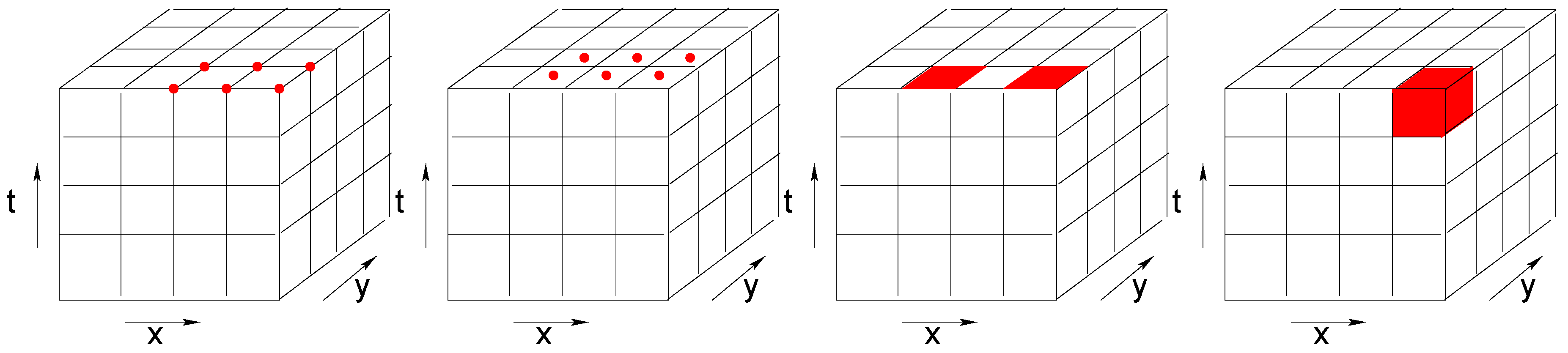
Depending on the studied phenomena and on the generation of the data, array cells may have different interpretations. As illustrated in Figure 1, they may represent point values, areal values that are constant within a cell (e.g., land use), or aggregations such as counts or averages (e.g., average intensity of reflected light). The same challenge applies to the time dimension. A time interval can reflect a temporal snapshot, an aggregation over a time period, or a constant value over a time period.
Taking the different levels of imagery products from optical remote sensing as an example, the energy of the Earth’s surface is recorded by forwarding the field of view of a imaging mechanism along the satellite’s orbit [17]. The swath recorded is divided into pixels. At all the levels the grid cell refers to the radiation that is gathered in each wavelength aggregated over each pixel. Each time interval of the level 0 data represents a time snapshot. At higher product levels, a regular timestamp is assigned to each imagery to correct the swath overlapping and to composite the best quality imagery. The time interval of high level products thus represents aggregation (by selection or averaging) over a time period.
Grid cells that represent a constant areal value are often seen when the variable is categorical, such as gridded land-cover land-use classification maps. Similarly, values of survey data may remain stable over a period of time.
3. Array Operations
Since arrays are functions, operations to modify array data can be formulated in the context of array algebras. Schmidt [18] presents a simple algebra and defines a few basic operations following relational algebra [19]. Array algebras are primarily used in designing database query languages [16,20,21]. These languages are then used in practice by data analysts. We reviewed algebra definitions [16,20,21,22] and software systems (Section 4) and present a categorisation of array operations based on whether they change dimensionality and whether the amount of data reduces, increases, or stays the same. We thereby concentrate on unary operations, i.e., operations that take a single input and produce a single output array. These operations are often needed in preprocessing data for analyzes. For instance, two-dimensional matrices must be constructed from higher dimensional data in many cases or the spatial or temporal resolution of the data must be homogenised to be compatible with other data. We categorised array operations into five types of operations (Figure 2), namely select, scale, reduce, rearrange and compute operations. Figure 2 shows the alterations of array shapes before and after applying these operations.
3.1. Select Operations
Select operations filter array cells by predicates. They involve both select and project operations from relational algebra [19] and work on attribute as well as on dimensions values. Typical applications include range queries on space and/or time, filtering cells whose attribute values meet certain conditions, and slicing arrays e.g., to extract a temporal snapshot of remote sensing image time series. Select operations may or may not decrease the number of dimensions and attributes of an array.
3.2. Scale Operations
Scale operations do not reduce the number of dimensions but the number of cells along one or more dimensions. Typical examples include spatial or temporal upscaling, such as computing daily mean values of hourly time series or downscaling climate model output. Any operation that involves resampling reduces the amount of information and thus can be categorised as a scale operation. Reprojecting spatial data is one example that introduces errors by resampling. Scale operations are generally meaningful only along dimensions with physical interpretation. In contrast, it is unclear how upscaling observations over the dimensions “sensor index” or “record id” can be reasonably interpreted. Scale operations are an important building block to homogenise datasets with different spatial and/or temporal resolution. Specific scale operations must address the support of array cells. Depending on whether cells represent point observations, aggregations, or constant values, applicable interpolation methods vary (e.g., point vs. block Kriging). Besides downscaling and upscaling, scale operations may introduce empty cells and thus might increase sparsity of arrays.
3.3. Reduce Operations
By applying an aggregation function along one or more dimensions, reduce operations decrease the number of dimensions and the total number of cells . They can be seen as an ultimate scaling where dimensions are completely dropped. The application of reduce operations yields meaningful results even for artificial dimensions. Specific aggregation functions could be simple statistics, such as the mean or the standard deviation as well as frequency distributions or even fits of theoretical models. Dimension reduction is an important task to extract relevant information and to make the data comprehensible and presentable.
3.4. Rearrange Operations
Rearrange operations change the dimensionality of an array without removing or aggregating any cells. They do not reduce the complexity inside datasets but offer an important degree of flexibility how to represent the data. The simplest rearrangement operation dimension flattening converts dimensions to attributes and adds a single artificial dimension like “record no.”, or “observation id”. This is equivalent to building a table or relation from multidimensional data. Flattening can be applied to subsets of array dimensions as well which is often applied to represent space in a single dimension (see Section 6.2 for an example). Similarly, n-dimensional arrays can be trivially embedded as slices in -dimensional arrays and attribute flattening reduces the number of attributes to one but adds an artificial dimension “attribute no.” Another important operation is reordering or permuting array dimensions or attributes.
A more general rearrange operation is the conversion from attributes to dimensions or vice versa. The former is always applicable but creates very sparse arrays in the general case while a subset of attributes can be converted to dimensions only if all attributes of V functionally depend on S. In analogy with the relational model, S must be a superkey of V whereas the conversion leads to cell conflicts and the rearrangement may involve a reduction otherwise.
The following array definitions illustrate typical examples how spatiotemporal data might be represented as arrays with different dimensionality. A, B, and C represent in situ sensor observation measurements, remote sensing imagery, and trajectories respectively. Subscript indexes present different possible schemas that can be flexibly rearranged by the mentioned operations.
3.5. Compute Operations
Simple compute operations derive new attributes based on existing attributes and dimensions. They do not change dimensionality but computations may include attribute values of other cells (e.g., neighbours in moving window operations).
4. Implementations
The implementation of array can be found in different data acquisition and analysing stages: array-based file formats and libraries (e.g., netcdf), programming languages for data analysis (e.g., R), data warehouses (e.g., OLAP, SOLAP), and databases for storage, access, and analysis (e.g., SciDB).
Programming languages, such as FORTRAN, C/C++, IDL, Matlab, Python, and R, support array data structure. We list array operations of three high-level data analytics and graphic systems, R, Matlab/Octave, Python, and array database management systems, Rasdaman and SciDB in Table 1. The table lists selected implemented array operations according to the categories described in Section 3. The amount of available compute operations strongly differs between data management systems and high-level analysis systems. The most generic multidimensional array model is implemented by SciDB and Rasdaman. They both support arbitrary amounts of dimensions and attributes. Refs. [23,24] extended SciDB and combine it with gdal to facilitate accessing and processing spatiotemporal data. For a similar goal, an extension of Rasdaman, Petascope [25], has been developed to handle spatial and temporal reference of arrays. ArrayUDF [10] is an UDF (User Defined Function) mechanism that optimizes operating UDFs on neighbouring cells of an array. With ArrayUDF, the shape of neighbourhoods to be processed can be flexibly defined instead of specifying a rectangular shape as is required for SciDB and Rasdaman, and each of the neighbouring cells are processed individually, indicating different algorithms can be applied to different neighbouring cells [10]. The Hadoop [26] distributed processing framework has been extended or optimized for array data querying and processing. For example, SciHadoop [27] is developed to avoid data conversion between array-based and Hadoop data models (HDFS) by allowing logical queries over array-based data models. Ref. [28] proposed a spatiotemporal indexing structure for grid partitian to link the logical (e.g., space, time) to physical location information(e.g., node, file). Base R, GNU Octave, and Python consider only a single attribute, multiple attributes can be represented as an additional dimension. In R, packages have been developed to facilitate manipulation of different types of spatiotemporal arrays. For example, the spacetime package [29] allows the spatiotemporal data to be indexed by space and time. Similarly, the raster package [30] is used to directly manipulate geographic data with the raster format. The packages are limited to 3 to 5 dimensions respectively but in terms of geographical analysis, they clearly proved the richest set of functionality.
5. Methods on Arrays
5.1. Regridding and Change of Support
A common operation on array data is regridding: deriving values for grid cells that are not aligned perfectly with the original grid cells. Regridding is particularly needed when data from different sources are integrated [31,32,33,34,35] or models acting at different grid configurations are combined, as in the CSDMS [4] or OpenMI [36] frameworks.
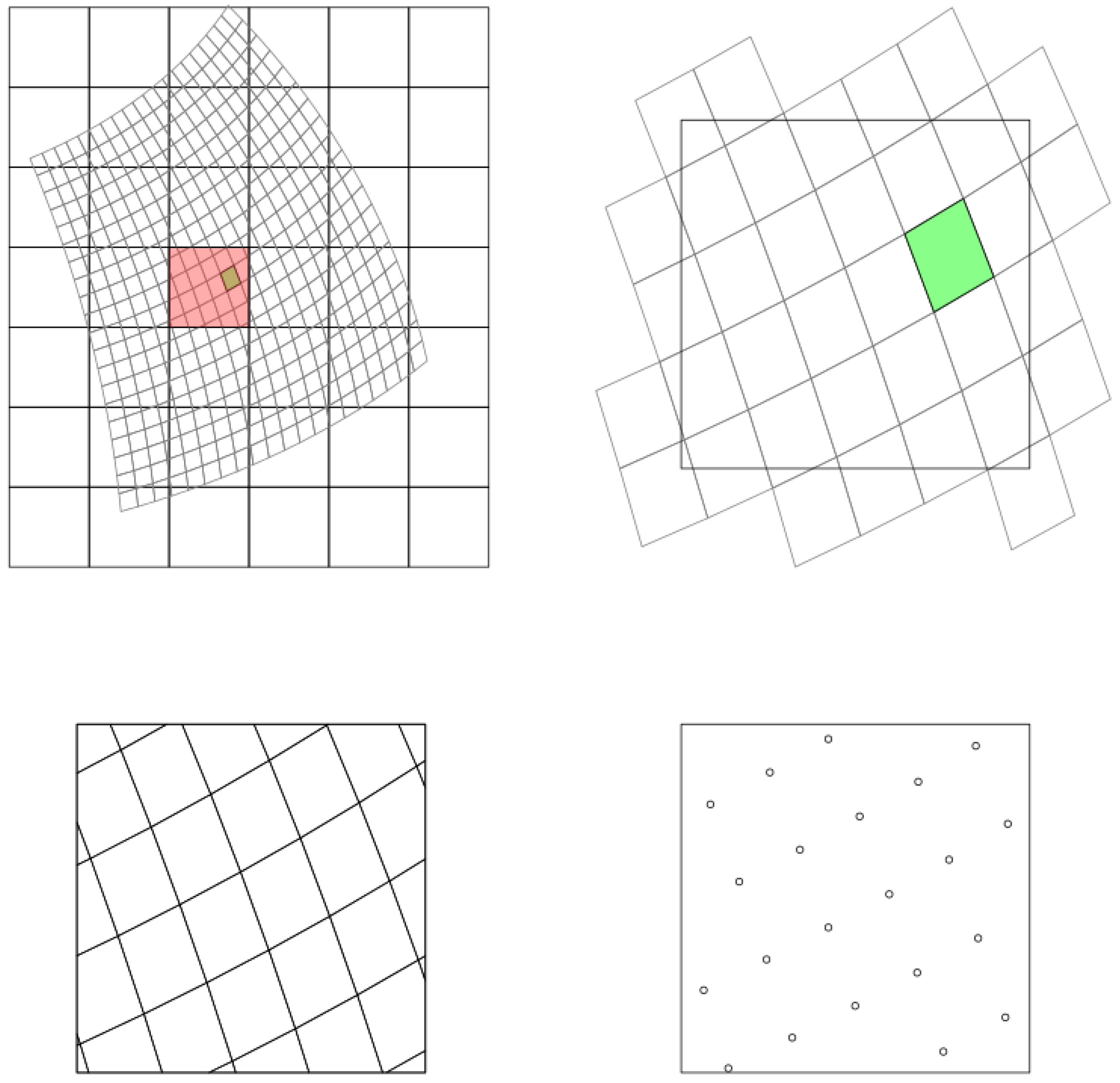
A utility that carries out regridding is gdalwarp, which is available as a binary executable and an API call in the GDAL library. This utility has 12 methods for obtaining new grid cell values. Several of these interpolate (nearest neighbour, bilinear, cubic, cubic spline, Lanczos windowed sinc [37]), others aggregate points covered by the new cell (Figure 3, lower right) using as aggregation function the average, mode, max, min, median, first quartile, or third quartile. None of the methods provides the aggregation of intersecting grid cell sections, such as depicted in the lower-left of Figure 3.
Which regridding method is most appropriate primarily depends on the measurement scale [38] of the regridded variable: if it is on a nominal scale (such as land use type), only nearest neighbour and mode are meaningful. If the origin grid cells are considered as points, and are much larger than the destination grid cells (Figure 3: regrid from the black to the grey cells) then interpolation methods make sense. If the origin grid cells are much smaller and aggregate values over the target cells (black cell in Figure 3) are needed, then aggregation methods make more sense. In any case, geostatistical methods for regridding are preferred because they adopt and parametrise an explicit model for the spatial variation of the variable being regridded [39,40]; they also allow for addressing grid points or cells outside the target grid cell for optimal spatial prediction, and cope with change of support, the dependence of variability of cell aggregated values on the aggregation area [41].
Regridding in the time dimension involves the same procedures as in space, and needs aggregation or disaggregation, possibly using smoothing methods. The temporal information may be associated with time instances, constants over time intervals, or aggregates over time intervals. For both spatial and temporal regridding, information gets lost: from the regridded information alone, typically the original information cannot be recovered.
5.2. Dimension Reduction
High dimensional data often contains redundant information, which mixes with the signals and is burdensome to computation and data storage. Such redundancy can be reduced with aggregation and feature extraction methods to turn the complex process to lower orders, so that useful information can be extracted or displayed. Aggregation and feature extraction are typical array functions that respectively reduce the dimensionality and cardinality of an array. Feature extraction methods linearly transform dependent variables to independent variables.
We briefly review a group of spatiotemporal feature extraction methods that are based on PCA (Principal Component Analysis). PCA is a classic orthogonal feature extraction method that is computed with singular vector decomposition (SVD) of the data matrix or an eigen decomposition of the covariance matrix. The ordering of columns and rows of a matrix for PCA is not pertinent; however, depending on the applications, the matrix can be ordered for a meaningful analysis. In remote sensing image processing, classification, atmospheric and meteorologic studies, PCA has been extended to concern space and time. For instances, the spatial dimension of a matrix is ordered in the MNF (Maximum Noise Fraction, [8]) to utilise the spatial correlation for noise estimation before applying PCA on a noise-to-signal ratio to isolate noise. EOFs (Empirical Orthogonal Functions), the discrete form of PCA, has been applied to ordered spatial or temporal dimensions to analyze the pattern or fluctuation in space or time. The temporal dimension is ordered in the Complex Hilbert EOF analysis to study the evolving of the spatial pattern along time, i.e., wave propagation. Similar to the complex Hilbert EOF, the POP (Principal Oscillation Pattern) analysis models the cyclical patterns of spatial time series by applying singular value decomposition to the estimated parameters of an auto-regressive model. Moreover, multiple response variables can be analyzed with multivariate EOF and CCA (Canonical Correlation Analysis). For example, the MAD (Multivariate Alteration Detection, [42]) uses CCA to minimise correlation between two paired images to model change. The time dimension is ordered when the time lagged versions of multivariate EOF and CCA are used to study the EOF or canonical correlation patterns between fields at two time stamps. In Section 6.2, we describe a study case that applies PCA to extract information from a multi-spectral spatiotemporal data. The array operations that were used in the study case and the corresponding functions in R and SciDB are shown.
6. Study Cases of Regridding and Dimension Reduction
6.1. Study Case: Regridding
This study case is developed to show the role of array regridding in integrating satellite images from different resolution and projections, and compare the results of same regridding functions implemented in different software. As is reviewed in Section 5.1, various regridding methods are implemented and in different software. Does the same regridding method implemented in different software obtain the same results, and do different regridding methods make a significant difference?
Satellites are designed with different spatial and temporal resolutions depending on their missions. A high spatial or temporal resolution is achieved with a compensation of the other. For example, satellites operating at low altitudes are capable of capturing details on Earth surface, but low revisiting frequency and global coverage as the swath widths of these sensors are narrow. Consequently, integrating satellite imagery products has become important to obtain more spatiotemporal information. Regridding is required to bring satellite imagery grids of different sources to the same grid.
We compare different software implementations of regridding methods and different regridding methods with a study case that reproject and align the grid of Landsat 8 (16-day, 30 m resolution, UTM projection) to the grid of MODIS 09Q1 product (8-day, 250 m resolution, Sinusoidal projection) of same location and time. The red bands of both products are used and are cropped to San-Diego city.
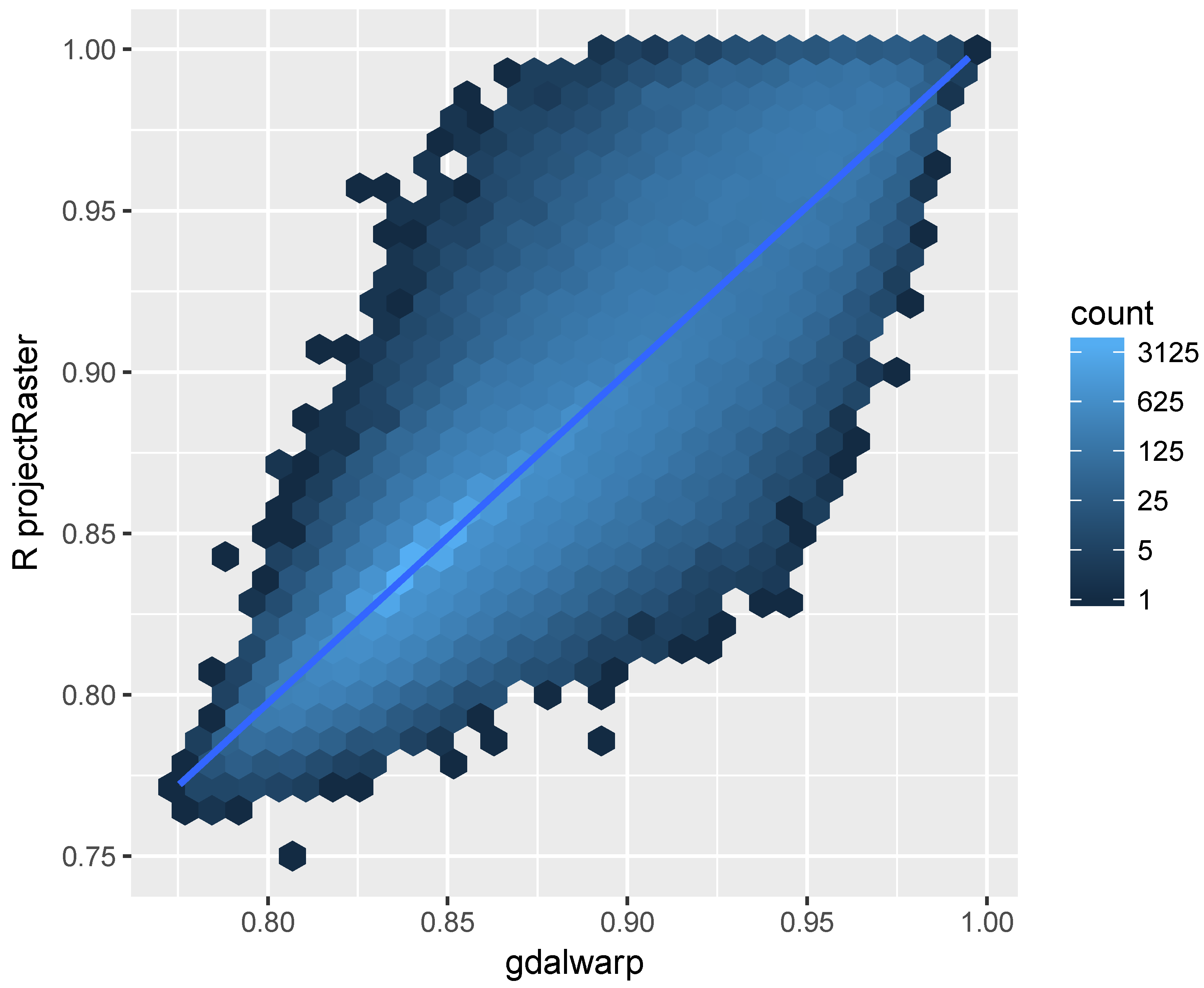
We compared the results of converting the landsat UTM grid to MODIS sinusoidal grid using the gdalwarp and projectRaster of the R raster package. For both methods, the bilinear interpretation is used for the resampling process. After reprojecting, the resample function of the R raster package is used to aggregate the Landsat 8 grid cells and register them to the MODIS grid. We regrid the near-infrared band reflectance of the Landsat 8 grid and filtered out pixels that are beyond the valid reflectance range (valid range: 0–1).
The result is shown in Figure 4, which indicates similar results obtained for the majority pixels using projectRaster and gdalwarp. However, the disparity between the two implementations are not trivial and it is higher for pixels with high reflectance. Same as gdalwap, the projectRaster converts between coordinates using the PROJ.4 library [43]. Therefore, the different reprojection results showed in Figure 4 may be due to the differences in implementations of the bilinear resampling in gdalwarp and projectRaster, the later uses an doBilinear function implemented in the raster package for the bilinear interpolation. The bilinear resampling in gdal is implemented in an GWKBilinearResample function.
The projectRaster includes two methods: bilinear and nearest neighbour. We compared these two methods to project and align the landsat 8 near infrared band to the MODIS grid. Figure 5 indicates the differences obtained using these two methods. The result of using bilinear and nearest neighbour methods are more consist comparing to the regridding results using two different software as is shown in Figure 4.
We compared the CPU times for code execution of the gdalwarp bilinear resampling, the projectRaster bilinear resampling, and the projectRaster nearest neighbour resampling. The CPU times for execution is measured using the “user time” returned from the R function proc.time. We repetitively ran the resampling process for each method 30 times and the shortest times for projectRaster bilinear, projectRaster nearest neighbour, and gdalwarp bilinear resampling are respectively: 0.19 s, 0.25 s, and 0.05 s, indicating the gdalwarp bilinear is computed faster than the projectRaster bilinear, and the projectRaster nearest neighbour takes longer to compute than the projectRaster bilinear method.
6.2. Study Case: Dimension Reduction
To show how PCA introduced in Section 5.2 can be applied to extract information from different array rearrangement of multidimensional data, and to show how array data structure, operations and software contribute to a clean and scalable multidimensional data analyzing process, we develop a study case that explores spatiotemporal change information from Earth observations. The study case applies PCA to Landsat (TM and ETM+) image time series. The study area is a subset (23.3 ha) of a pine plantation field located in Lautoka, Fiji (17.34 S, 177.27 E, 9570 ha), where detailed forest inventory data is available [32,44]. The plantations in the study area were logged on 27 May 2010 and were immediately replanted. The Landsat TM and ETM+ scenes (Path 75, Row 72) from 2000 to 2010 (, ) were downloaded and cropped. Pixels containing clouds and cloud shadows were masked using an Fmask (Function of mask) [45] and were considered as missing values. The cropped and preprocessed images that contain more than 50% of missing values are removed. The Dimensionality of the final 4-d array is .
As PCA works on 2-d matrices, different composites of dimensions are rearranged from the 4-d array. The matrices are formed as:
- bands are variables (columns), temporal-spatial points are observations ()
- times are variables, spectral-spatial points are observations ()
- spectral time series are variables, spatial points are observations ()
For each matrix, the variables are scaled (column mean subtracted and divided by column standard deviation).
Principal Component (PC) loadings are the coefficients of original variables forming the PCs variables, and can be seen as the correlations between the original variables and the PC components. Therefore, the patterns of PC loadings of each PC component may reveal i.e., change information from matrices with spatial, spectral and temporal dimensions.
The loadings of the first PC (PC1) and the second PC (PC2) of (Figure 6a) show a distinction, i.e., low correlation, between band 4 (near infrared) and the other bands (bands 1–3, 5, and 7), which may be explained by the different vegetation reflectance exhibited by band 4 and the other bands. The PC loadings of the are shown in Figure 6b. PC1 may indicate the brightness of the area since the correlation between all the spectral partial bands at each time are similarly strong. PC2 shows a contrast between the times before and after 27 May 2010, which is explained by the harvesting event. The PC loadings of (Figure 6c) reveal spectral temporal information. Between each two grey, dashed lines are the PC loadings of the time series of a spectral band. The brown line indicates the time when the deforestation occurred. The PC1 loadings may indicate general brightness, the spatial points of time stamps show positive correlations between most of the spatial points of time stamps of each band. The spatial points of a few time stamps that are negatively correlated with other time stamps are at the time when the deforestation event occurred. PC2 shows that the reflectance at all the time stamps of band 4 are positively correlated (the band 4 of PC2 shows the same pattern as other bands of PC1). For other bands, the PC loadings show the same direction after the deforestation event, the directions are different from most of the PC loadings before the deforestation event.
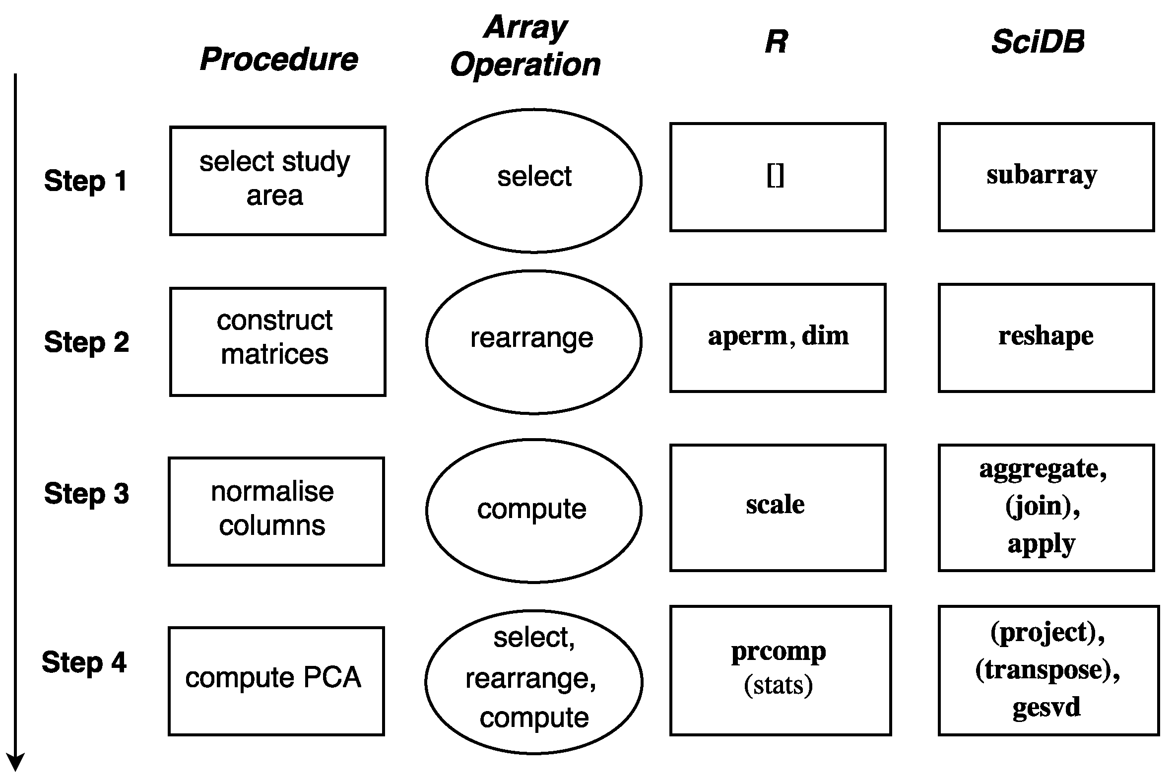
The procedure of the study case, the corresponding array operations, and the functions that are used in R and SciDB in each step are shown in Figure 7. The implementation in SciDB requires additional join and project steps due to the multi-attribute storage feature of SciDB. The scripts are available at https://github.com/ifgi/rearrange.
7. Discussion
This paper emphasizes arrays for representing spatiotemporal phenomena to analyze geoscientific data. Arrays discretise continuous spatiotemporal phenomena, where grid cell values reflect point values, grid cell aggregates, or constant values over grid cells. Constant valued cells are relevant for phenomena that have a categorical measurement scale. As was mentioned in Section 2.3, the arrays of raw optical satellite images aggregate continuous spatial phenomena and sample the time: grid cells reflect an aggregation over a region for a given time stamp. Arrays may aggregate continuous temporal phenomena and sample the locations, such as arrays of monthly average rainfall amounts gathered from rainfall gauge networks. In this case, the array cells convey aggregation over a time interval at a spatial location. Arrays may also sample locations and times, with most in situ sensors being examples. The array cells here indicate a point in space and time: although physical constraints imply that every measurement must have a size and duration, in the context of the extent of the measurements we conceive them as point measurements.
We categorised array operations and list their implementation in several open-source software environments in Table 1. These environments not only offer quite different functionality, they also use very different names for identical operations, which complicates the comparison of analysis scripts developed for different environments. Also, there are strong differences in support for sparse and irregular arrays, as well as to the extent they scale up for analysing massive data. None of the systems considered support to register or query whether grid cell values refer to grid cell aggregates, constants, or point values, even if this is information obvious from the operation used to compute an array.
We illustrated the challenges from multidimensional data analysis in array applications. Array regridding has implications in satellite image registration, array data up-/down-scaling, missing data interpolation, and multi-source data fusion. It is worth noting that a change of support [46] may be caused by the array regridding process.
Arrays naturally store geoscientific data with the order and the neighbourhood information preserved, which may facilitate multidimensional information integration [47]. Analysing spatiotemporal information jointly, rather than first analysing space and then time or vice-versa, may result in more effective use of multidimensional information [5]. Spatiotemporal analysis methods commonly either focus on spatial pattern/feature over time, or the time series structure of each location over space [5]. The separate analyzes in space and time lose joint spatiotemporal information [48] and may lead to an uninterpretable modeling process [5]. Joint spatiotemporal statistical methods [49,50,51] address the spatiotemporal modeling problems by building hierarchical models or jointly accounting for spatiotemporal dependency. In addition, rich data are needed for the complex spatiotemporal modeling process, which often requires multi-source data integration. Developing multidimensional information extracting methods and applying them to solve real-life problems remain a challenge in array modeling.
Dimension reduction methods (such as principle component analysis) apply to a matrix, where the ordering of columns and rows is irrelevant. The dimensions of a matrix can be ordered to extract spatiotemporal information for specific purposes (e.g., POP). A study case is given to illustrate how dimension reduction methods can reveal important information from different rearrangement of multidimensional arrays, and shows how array operations are applied to accomplish this.
The array model facilitates going from high-dimensional data to matrix-based statistical analyzes. At the same time, the array model presents an efficient organization of geoscientific datasets. Array dimensions, such as space and time, define distances between cells which can be used to store nearby observations at nearby locations in computer memory or on hard disks. Array partitioning as implemented in SciDB [11] and Rasdaman [12] also facilitates the data distribution in large distributed computing environments in order to balance computational load and memory consumption. However, the choice of the order of dimensions and the partitioning schema may have a strong impact on computation times and often needs consideration.
Much progress has been made [11,52] to store sparse arrays with minimum memory consumption. Analysing sparse and irregular arrays remains a challenge. For instance, if a sparse array is used to store an irregular spatial array, the cell size of the data can no longer be computed from the sequence of spatial index values (e.g., Northing and Easting, [53]). Irregular dimensions of an array may confine the application of many spatiotemporal statistical methods that were designed for regular data. Regularising the irregular arrays by aggregation or interpolation may come at the cost of accuracy and resolution. In addition, treating a sparse array as dense when applying an algorithm will greatly increase the workloads. Statistical methods that concern irregular or sparse time series [54,55,56] and sparse spatial arrays [50,57] have been developed. These methods often come with added complexity and restrain, making their application less general. Furthermore, the irregularity may lead to improper statistical methods to be used. For example, an empirical orthogonal function (EOF) decomposition of observation locations with irregularly spaced area without considering the relative area leads to misinterpretation of the results [49].
Arrays are a type of DGGs (Discrete Global Grids). Bauer-Marschallinger et al. [3] proposed a regular grid called Equi7 and concluded that projecting with the Equi7 grid causes the least geometric distortion compared to the global and hemispherical grids. Irregular grids polygons and meshes from other DGGs [58,59] may provide a more accurate projection of the spherical data; but will add difficulties in storing and analysing array data.
This study shows arrays to be a convenient data structure to apply multidimensional algorithms and shows the potential of arrays as a uniform data structure to handle big geoscientific data. The increasing use of Earth observations calls for solutions to the array challenges we mention in this paper: the semantics of grid cell values, regridding, information integration and dimension reduction. In many applications, other data types such as meshes, tables, polygons, may more efficiently represent spatiotemporal phenomena.
Author Contributions
Conceptualization: M.L., M.A., E.P. The coauthors have their contributions of writing in different sections. Specifically, M.L. wrote Section 5, Section 6 and Section 7 and the second part of Section 1, part of Section 2 and Section 4. M.A. wrote Section 3 and major parts of Section 2 and Section 4. E.P. wrote the first part of Section 1 and Section 5.1. Experimental conducting: M.L. Paper constructing and editing: M.L.
Funding
This research received no external funding.
Acknowledgments
The Fiji pine plantation reference data that is used in the study case is collected by Johannes Reiche from Wageningen University. We are grateful to him for offering the data.
Conflicts of Interest
The authors declare no conflict of interest.
Abbreviations
The following abbreviations are used in this manuscript:
| DGGs | Discrete Global Grids |
| PCA | Principal Component Analysis |
| EOF | Empirical Orthogonal Functions |
| MNF | Maximum Noise Fraction |
| CCA | Canonical Correlation Analysis |
| Fmask | Function of mask |
| SVD | Singular Vector Decomposition |
| UTC | Coordinate Universal Time |
References
- Galton, A. Fields and objects in space, time, and space-time. Spat. Cogn. Comput. 2004, 4, 39–68. [Google Scholar] [CrossRef]
- Scheider, S.; Gräler, B.; Pebesma, E.; Stasch, C. Modelling spatio-temporal information generation. Int. J. Geogr. Inf. Sci. 2016, 30, 1980–2008. [Google Scholar]
- Bauer-Marschallinger, B.; Sabel, D.; Wagner, W. Optimisation of global grids for high-resolution remote sensing data. Comput. Geosci. 2014, 72, 84–93. [Google Scholar] [CrossRef]
- Peckham, S.D.; Hutton, E.W.; Norris, B. A component-based approach to integrated modeling in the geosciences: The design of CSDMS. Comput. Geosci. 2013, 53, 3–12. [Google Scholar] [CrossRef]
- Schabenberger, O.; Gotway, C.A. Statistical Methods for Spatial Data Analysis; CRC Press: Boca Raton, FL, USA, 2004. [Google Scholar]
- Gotway, C.A.; Young, L.J. Combining incompatible spatial data. J. Am. Stat. Assoc. 2002, 97, 632–648. [Google Scholar] [CrossRef]
- Hyvärinen, A. Survey on independent component analysis. Neural Comput. Surv. 1999, 2, 94–128. [Google Scholar]
- Green, A.A.; Berman, M.; Switzer, P.; Craig, M.D. A transformation for ordering multispectral data in terms of image quality with implications for noise removal. IEEE Trans. Geosci. Remote Sens. 1988, 26, 65–74. [Google Scholar] [CrossRef] [Green Version]
- Furtado, P.; Baumann, P. Storage of multidimensional arrays based on arbitrary tiling. In Proceedings of the 15th International Conference on Data Engineering, Sydney, Australia, 23–26 March 1999; pp. 480–489. [Google Scholar]
- Dong, B.; Wu, K.; Byna, S.; Liu, J.; Zhao, W.; Rusu, F. ArrayUDF: User-Defined Scientific Data Analysis on Arrays. In Proceedings of the 26th International Symposium on High-Performance Parallel and Distributed Computing, Washington, DC, USA, 26–30 June 2017; ACM: New York, NY, USA, 2017; pp. 53–64. [Google Scholar]
- Stonebraker, M.; Brown, P.; Zhang, D.; Becla, J. SciDB: A database management system for applications with complex analytics. Comput. Sci. Eng. 2013, 15, 54–62. [Google Scholar] [CrossRef]
- Baumann, P.; Dehmel, A.; Furtado, P.; Ritsch, R.; Widmann, N. The Multidimensional Database System RasDaMan; ACM SIGMOD Record; ACM: New York, NY, USA, 1998; Volume 27, pp. 575–577. [Google Scholar]
- Rusu, F.; Cheng, Y. A survey on array storage, query languages, and systems. arXiv, 2013; arXiv:1302.0103. [Google Scholar]
- Cudre-Mauroux, P.; Kimura, H.; Lim, K.-T.; Rogers, J.; Madden, S.; tonebraker, M.; Zdonik, S.B.; Brown, P.G. Ss-db: A Standard Science DBMS Benchmark. Available online: www-conf.slac.stanford.edu/xldb10/docs/ssdb_benchmark.pdf (accessed on 2 August 2018).
- Cheng, Y.; Rusu, F. Formal representation of the SS-DB benchmark and experimental evaluation in EXTASCID. Distrib. Parallel Datab. 2015, 33, 277–317. [Google Scholar] [CrossRef]
- Baumann, P. A database array algebra for spatio-temporal data and beyond. In Next Generation Information Technologies and Systems; Springer: Berlin, Germany, 1999; pp. 76–93. [Google Scholar]
- Richards, J.A.; Jia, X. Remote Sensing Digital Image Analysis: An Introduction; Springer-Verlag, Inc.: Secaucus, NJ, USA, 2005. [Google Scholar]
- Schmidt, A. An Array Algebra. arXiv, 2008; arXiv:0812.4986. [Google Scholar]
- Codd, E.F. A relational model of data for large shared data banks. Commun. ACM 1970, 13, 377–387. [Google Scholar] [CrossRef]
- Marathe, A.P.; Salem, K. A Language for Manipulating Arrays. In Proceedings of the 23rd International Conference on Very Large Data Bases VLDB ’97, Athens, Greece, 25–29 August 1997; Morgan Kaufmann Publishers Inc.: San Francisco, CA, USA, 1997; pp. 46–55. [Google Scholar]
- Van Ballegooij, A. RAM: A Multidimensional Array DBMS; EDBT Workshops; Springer: Berlin, Germany, 2004; Volume 3268, pp. 154–165. [Google Scholar]
- Ritter, G. Recent developments in image algebra. Adv. Electron. Electron Phys. 1991, 80, 243–308. [Google Scholar]
- Appel, M.; Lahn, F.; Pebesma, E.; Buytaert, W.; Moulds, S. Scalable Earth-observation Analytics for Geoscientists: Spacetime Extensions to the Array Database SciDB. In Proceedings of the EGU General Assembly 2016, Vienna, Austria, 17–22 April 2016; Volume 18. [Google Scholar]
- Appel, M.; Lahn, F.; Buytaert, W.; Pebesma, E. Open and scalable analytics of large Earth observation datasets: From scenes to multidimensional arrays using SciDB and GDAL. ISPRS J. Photogramm. Remote Sens. 2018, 138, 47–56. [Google Scholar] [CrossRef]
- Aiordăchioaie, A.; Baumann, P. Petascope: An open-source implementation of the OGC WCS Geo service standards suite. In Proceedings of the International Conference on Scientific and Statistical Database Management, Portland, OR, USA, 20–22 July 2011; Springer: Berlin, Germany, 2010; pp. 160–168. [Google Scholar]
- White, T. Hadoop: The Definitive Guide; O’Reilly Media, Inc.: Newton, MA, USA, 2012. [Google Scholar]
- Buck, J.B.; Watkins, N.; LeFevre, J.; Ioannidou, K.; Maltzahn, C.; Polyzotis, N.; Brandt, S. SciHadoop: Array-based query processing in Hadoop. In Proceedings of the 2011 International Conference for High Performance Computing, Networking, Storage and Analysis, Washington, DC, USA, 12–18 November 2011; pp. 1–11. [Google Scholar]
- Li, Z.; Hu, F.; Schnase, J.L.; Duffy, D.Q.; Lee, T.; Bowen, M.K.; Yang, C. A spatiotemporal indexing approach for efficient processing of big array-based climate data with MapReduce. Int. J. Geogr. Inf. Sci. 2017, 31, 17–35. [Google Scholar] [CrossRef]
- Pebesma, E. spacetime: Spatio-temporal data in R. J. Stat. Softw. 2012, 51, 1–30. [Google Scholar] [CrossRef]
- Hijmans, R.J.; van Etten, J. Raster: Geographic Data Analysis and Modeling. R Package Version 2.5-8. Available online: https://CRAN.R-project.org/package=raster (accessed on 2 August 2018).
- Yue, L.; Shen, H.; Yuan, Q.; Zhang, L. Fusion of multi-scale DEMs using a regularized super-resolution method. Int. J. Geogr. Inf. Sci. 2015, 29, 2095–2120. [Google Scholar] [CrossRef]
- Reiche, J.; Verbesselt, J.; Hoekman, D.; Herold, M. Fusing Landsat and SAR time series to detect deforestation in the tropics. Remote Sens. Environ. 2015, 156, 276–293. [Google Scholar] [CrossRef]
- Sedano, F.; Kempeneers, P.; Hurtt, G. A Kalman Filter-Based Method to Generate Continuous Time Series of Medium-Resolution NDVI Images. Remote Sens. 2014, 6, 12381–12408. [Google Scholar] [CrossRef] [Green Version]
- Gevaert, C.M.; García-Haro, F.J. A comparison of STARFM and an unmixing-based algorithm for Landsat and MODIS data fusion. Remote Sens. Environ. 2015, 156, 34–44. [Google Scholar] [CrossRef]
- Schmidt, M.; Lucas, R.; Bunting, P.; Verbesselt, J.; Armston, J. Multi-resolution time series imagery for forest disturbance and regrowth monitoring in Queensland, Australia. Remote Sens. Environ. 2015, 158, 156–168. [Google Scholar] [CrossRef] [Green Version]
- Gregersen, J.; Gijsbers, P.; Westen, S. OpenMI: Open modelling interface. J. Hydroinform. 2007, 9, 175–191. [Google Scholar] [CrossRef]
- Duchon, C.E. Lanczos filtering in one and two dimensions. J. Appl. Meteorol. 1979, 18, 1016–1022. [Google Scholar] [CrossRef]
- Stevens, S.S. On the Theory of Scales and Measurement. Science 1946, 103, 677–680. [Google Scholar] [CrossRef] [PubMed]
- Bierkens, M.; Finke, P.; De Willigen, P. Upscaling and Downscaling Methods for Environmental Research; Kluwer Academic: Dordrecht, The Netherlands, 2000. [Google Scholar]
- Truong, P.N.; Heuvelink, G.B.; Pebesma, E. Bayesian area-to-point kriging using expert knowledge as informative priors. Int. J. Appl. Earth Obs. Geoinf. 2014, 30, 128–138. [Google Scholar] [CrossRef]
- Journel, A.G.; Huijbregts, C.J. Mining Geostatistics; Academic Press: Cambridge, MA, USA, 1978. [Google Scholar]
- Nielsen, A.A.; Conradsen, K.; Simpson, J.J. Multivariate alteration detection (MAD) and MAF postprocessing in multispectral, bitemporal image data: New approaches to change detection studies. Remote Sens. Environ. 1998, 64, 1–19. [Google Scholar] [CrossRef]
- PROJ contributors. PROJ Coordinate Transformation Software Library; Open Source Geospatial Foundation: Chicago, IL, USA, 2018. [Google Scholar]
- Reiche, J.; de Bruin, S.; Hoekman, D.; Verbesselt, J.; Herold, M. A Bayesian approach to combine Landsat and ALOS PALSAR time series for near real-time deforestation detection. Remote Sens. 2015, 7, 4973–4996. [Google Scholar] [CrossRef]
- Zhu, Z.; Woodcock, C.E. Object-based cloud and cloud shadow detection in Landsat imagery. Remote Sens. Environ. 2012, 118, 83–94. [Google Scholar] [CrossRef]
- Cressie, N. Statistics For Spatial Data, Revised Edition; John Wiley & Sons: New York, NY, USA, 1993; p. 928. [Google Scholar]
- Lu, M.; Pebesma, E.; Sanchez, A.; Verbesselt, J. Spatio-temporal change detection from multidimensional arrays: Detecting deforestation from MODIS time series. ISPRS J. Photogramm. Remote Sens. 2016, 117, 227–236. [Google Scholar] [CrossRef]
- Doherty, P.J.; Guo, Q.; Li, W.; Doke, J. Space-time analyses for forecasting future incident occurrence: A case study from Yosemite National Park using the presence and background learning algorithm. Int. J. Geogr. Inf. Sci. 2014, 28, 910–927. [Google Scholar] [CrossRef]
- Cressie, N.; Wikle, C.K. Statistics for Spatio-Temporal Data; John Wiley & Sons: Hoboken, NJ, USA, 2015. [Google Scholar]
- Bolin, D.; Lindström, J.; Eklundh, L.; Lindgren, F. Fast estimation of spatially dependent temporal vegetation trends using Gaussian Markov random fields. Comput. Stat. Data Anal. 2009, 53, 2885–2896. [Google Scholar] [CrossRef] [Green Version]
- Huang, B.; Wu, B.; Barry, M. Geographically and temporally weighted regression for modeling spatio-temporal variation in house prices. Int. J. Geogr. Inf. Sci. 2010, 24, 383–401. [Google Scholar] [CrossRef]
- Bates, D.; Maechler, M. Matrix: Sparse and Dense Matrix Classes and Methods. R Package Version 1.2-7.1. Available online: https://CRAN.R-project.org/package=Matrix (accessed on 2 August 2018).
- Planthaber, G.; Stonebraker, M.; Frew, J. EarthDB: Scalable analysis of MODIS data using SciDB. In Proceedings of the 1st ACM SIGSPATIAL International Workshop on Analytics for Big Geospatial Data, Redondo Beach, CA, USA, 6 November 2012; ACM: New York, NY, USA, 2012; pp. 11–19. [Google Scholar]
- Jones, R.H. Maximum likelihood fitting of ARMA models to time series with missing observations. Technometrics 1980, 22, 389–395. [Google Scholar] [CrossRef]
- Scargle, J.D. Studies in astronomical time series analysis. II-Statistical aspects of spectral analysis of unevenly spaced data. Astrophys. J. 1982, 263, 835–853. [Google Scholar] [CrossRef]
- Broersen, P.M.; Bos, R. Time-series analysis if data are randomly missing. IEEE Trans. Instrum. Meas. 2006, 55, 79–84. [Google Scholar] [CrossRef]
- Furrer, R.; Sain, S.R. spam: A Sparse Matrix R Package with Emphasis on MCMC Methods for Gaussian Markov Random Fields. J. Stat. Softw. 2010, 36, 1–25. [Google Scholar] [CrossRef]
- Sahr, K.; White, D.; Kimerling, A.J. Geodesic discrete global grid systems. Cartogr. Geogr. Inf. Sci. 2003, 30, 121–134. [Google Scholar] [CrossRef]
- Dutton, G.H. A Hierarchical Coordinate System for Geoprocessing and Cartography; Springer: Berlin, Germany, 1999. [Google Scholar]
Figure 1.
Different meaning of cells in spacetime arrays.

Figure 2.
Array operations, from top to bottom: select, scale, reduce, rearrange and compute operations. “A” indicates original arrays, “B” indicates result arrays after certain array operations are applied. The application of “reduce” functions changes array cardinality, the application of “rearrange" functions alters array dimensions.
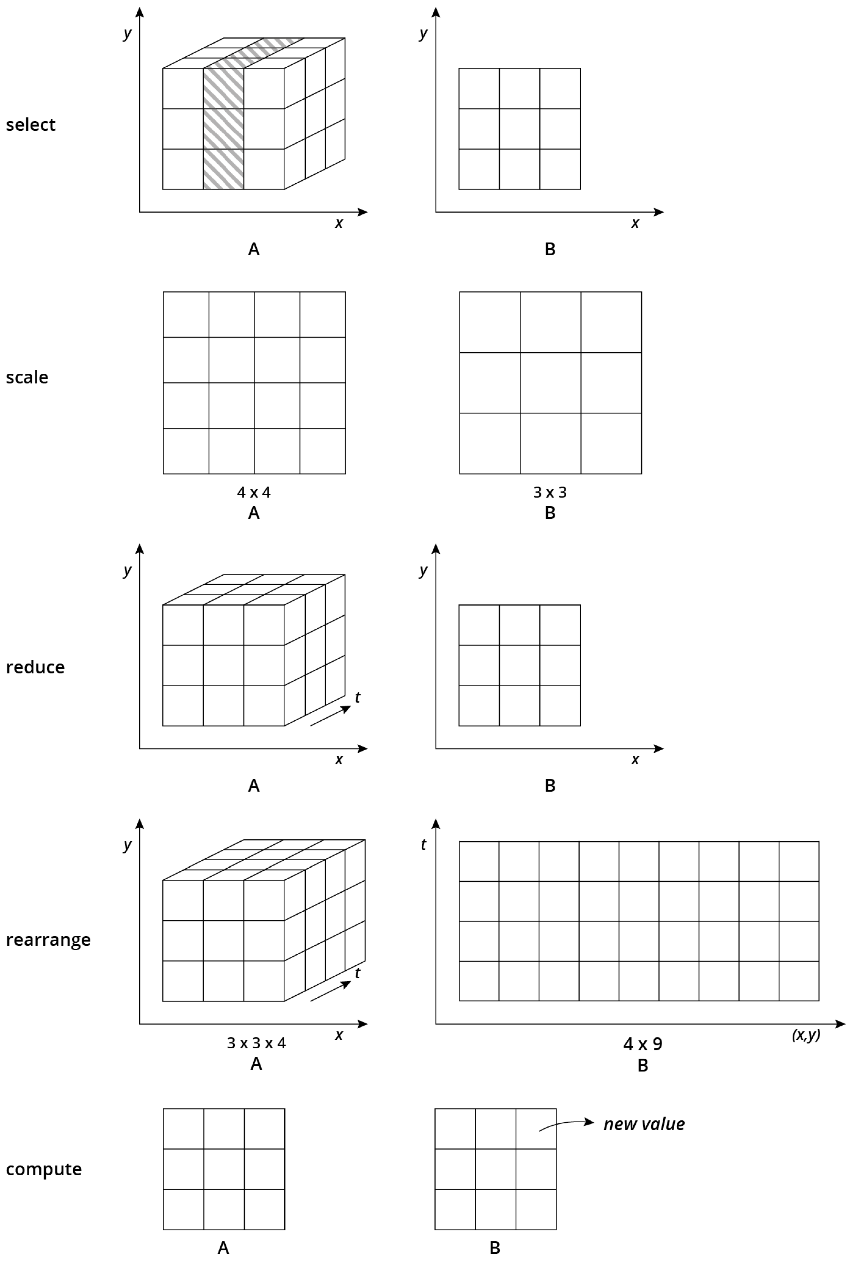
Figure 3.
Regridding: original values are available for the grid indicated by grey lines, new values are required for the black lined grid (e.g., the red cell), or vice versa (e.g., the green cell). New cell values can be calculated from the intersecting grid areas (lower left), intersecting grid cell centre points (lower right), or using interpolation (e.g., from black cells or cell center points to the green cell).

Figure 4.
Comparing using the bilinear resampling of projectRaster and gdalwarp to reproject and resample the grid of Landsat 8 image to the grid of the MODIS 09Q1 image.
Figure 4.
Comparing using the bilinear resampling of projectRaster and gdalwarp to reproject and resample the grid of Landsat 8 image to the grid of the MODIS 09Q1 image.

Figure 5.
A comparison between using the bilinear and the nearest neighbour methods to align the Landsat TM band to the MODIS grid.
Figure 5.
A comparison between using the bilinear and the nearest neighbour methods to align the Landsat TM band to the MODIS grid.
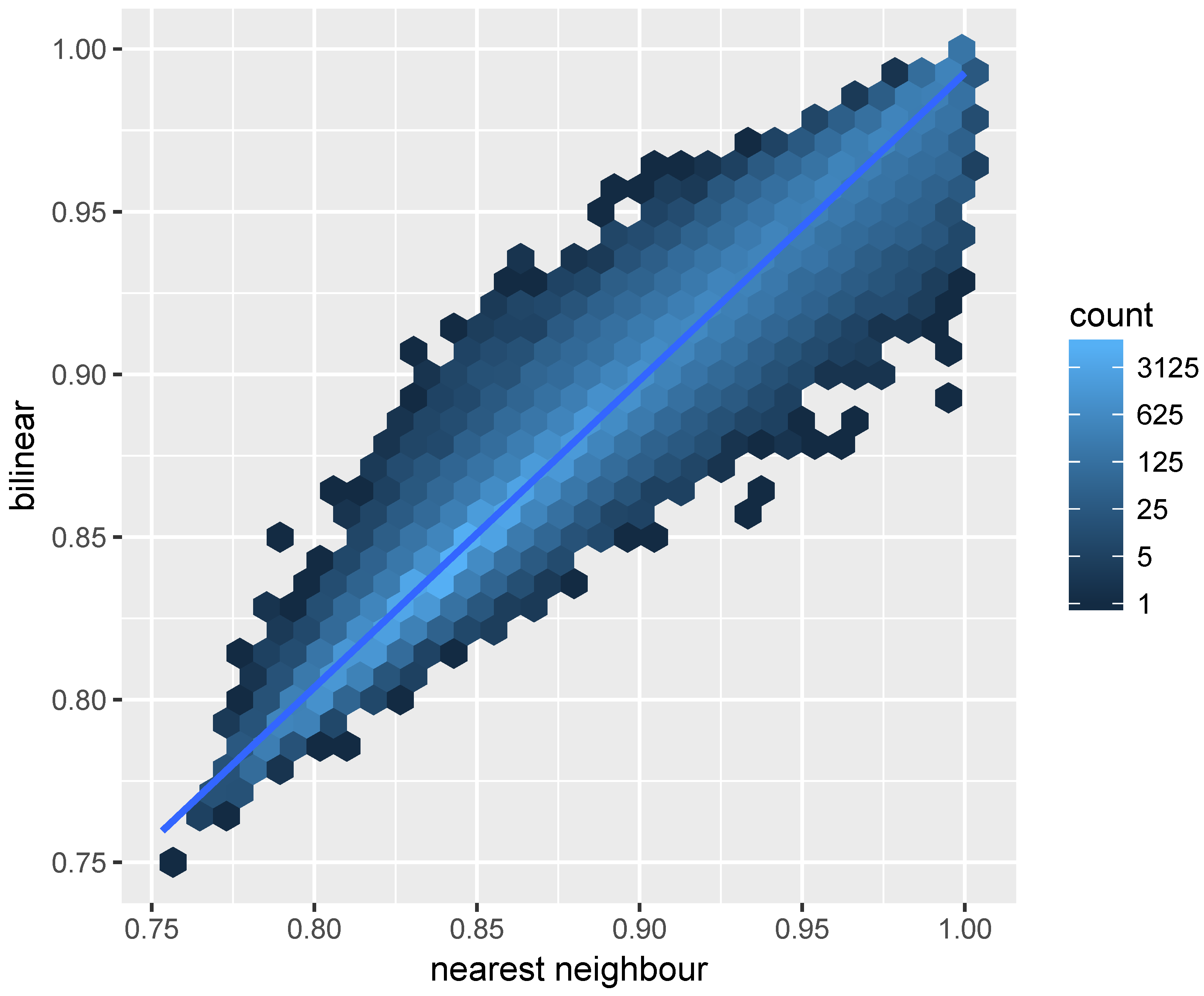
Figure 6.
PC loadings (1–4) of (a), (b) and (c). The brown vertical line indicates the time of the harvesting event. The points between two grey vertical lines are spatial points of a spectral band.
Figure 6.
PC loadings (1–4) of (a), (b) and (c). The brown vertical line indicates the time of the harvesting event. The points between two grey vertical lines are spatial points of a spectral band.
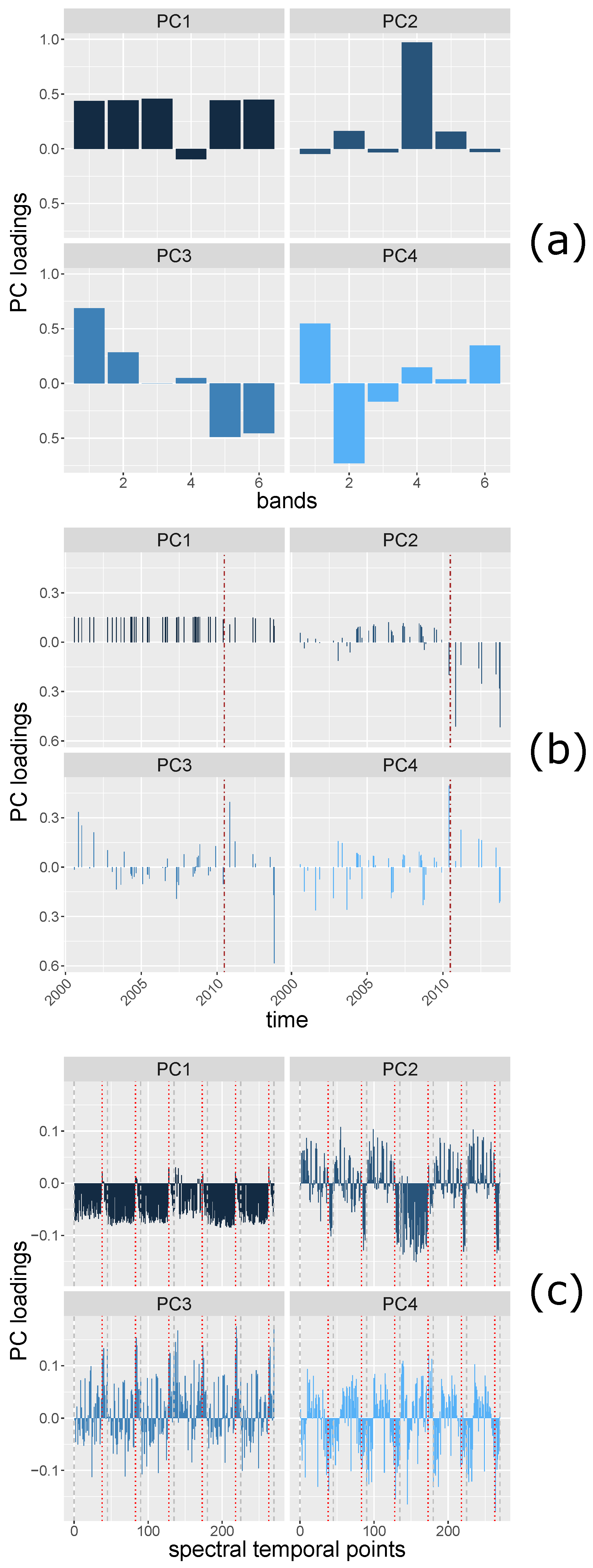
Figure 7.
The procedure of the study case and the corresponding array operations, R and SciDB functions.
Figure 7.
The procedure of the study case and the corresponding array operations, R and SciDB functions.

Table 1.
Comparison of natively supported array operations in open-source data analysis software. UDF indicates user defined functions. Support of specific features is encoded as single letters where: 0 and I indicate support of sparse storage and irregular array dimensions respectively, G denotes whether geographic dimensions (space, time) are handled explicitly, and S represents whether the support of cells is considered appropriately. and are the maximum number of dimensions and attributes with n and m the limits, absence indicates no limits. LA indicates that linear algebra routines for vectors and matrices are available.
| Features | Select Operations | Scale Operations | Reduce Operations | Rearrange Operations | Compute Operations | |
|---|---|---|---|---|---|---|
| R (base) | , LA | [] which | apply | apply | aperm dim <- t as | apply +,−,*,/ !,&&,|| ... |
| R (raster) | G,, | [] crop which | aggregate disaggregate calc resample | calc | as | focal calc +,-,*,/ !,&&,|| ... |
| R (spacetime) | S,0,G, I, | [] | aggregate | apply | as | +,-,*,/ !,&&,|| ... |
| GNU Octave | , LA | , [] | accumarray sum prod sumsq | reshape permute ipermute vertcat horzcat flipud flip rot90 rotdim vec | arrayfun cumsum cumprod +,-,*,/ not,and,or ... | |
| Python (NumPy) | , LA | [] take clip | apply_ over_axes apply_ along_axes | min max trace prod sum mean var std apply_ over_axes apply_ along_axes | flatten ravel swapaxes transpose reshape resize squeeze | cumsum cumprod +,-,*,/ not,and,or ... |
| Rasdaman CE (RASQL) | G | select where [] . | scale | condense | +,-,*,/ not,and,or ... | |
| SciDB CE (AFL) | 0,G,LA | subarray between project filter slice | regrid xgrid | aggregate | redimension reshape transpose | window cumulate +,-,*,/ apply not,and,or ... |
| ArrayUDF | G | UDF | UDF | UDF | UDF | UDF |
© 2018 by the authors. Licensee MDPI, Basel, Switzerland. This article is an open access article distributed under the terms and conditions of the Creative Commons Attribution (CC BY) license (http://creativecommons.org/licenses/by/4.0/).
Share and Cite
MDPI and ACS Style
Lu, M.; Appel, M.; Pebesma, E. Multidimensional Arrays for Analysing Geoscientific Data. ISPRS Int. J. Geo-Inf. 2018, 7, 313. https://doi.org/10.3390/ijgi7080313
AMA Style
Lu M, Appel M, Pebesma E. Multidimensional Arrays for Analysing Geoscientific Data. ISPRS International Journal of Geo-Information. 2018; 7(8):313. https://doi.org/10.3390/ijgi7080313
Chicago/Turabian StyleLu, Meng, Marius Appel, and Edzer Pebesma. 2018. "Multidimensional Arrays for Analysing Geoscientific Data" ISPRS International Journal of Geo-Information 7, no. 8: 313. https://doi.org/10.3390/ijgi7080313
Note that from the first issue of 2016, this journal uses article numbers instead of page numbers. See further details here.