Mapping Urban Land Use at Street Block Level Using OpenStreetMap, Remote Sensing Data, and Spatial Metrics

Abstract

Up-to-date and reliable land-use information is essential for a variety of applications such as planning or monitoring of the urban environment. This research presents a workflow for mapping urban land use at the street block level, with a focus on residential use, using very-high resolution satellite imagery and derived land-cover maps as input. We develop a processing chain for the automated creation of street block polygons from OpenStreetMap and ancillary data. Spatial metrics and other street block features are computed, followed by feature selection that reduces the initial datasets by more than 80%, providing a parsimonious, discriminative, and redundancy-free set of features. A random forest (RF) classifier is used for the classification of street blocks, which results in accuracies of 84% and 79% for five and six land-use classes, respectively. We exploit the probabilistic output of RF to identify and relabel blocks that have a high degree of uncertainty. Finally, the thematic precision of the residential blocks is refined according to the proportion of the built-up area. The output data and processing chains are made freely available. The proposed framework is able to process large datasets, given that the cities in the case studies, Dakar and Ouagadougou, cover more than 1000 km² in total, with a spatial resolution of 0.5 m.

1. Introduction

As reported by the United Nations, urban areas currently contain more than 50% of the world’s population. According to the latest estimates, this proportion will reach 60% by 2030 [1]. In developing countries, high urbanization rates and uncontrolled urban sprawl often lead to challenges such as inefficiency of transport systems, degradation of the environment, growth of informal settlements, and a proportion of the population living in deprived conditions. Availability of accurate and up-to-date information about the current situation of a city could help in defining and setting up adapted urban policies.

Among the set of potential geospatial information related to urban areas, population density and land use are probably the most important to an urban planner [2]. Unfortunately, they are limited or not available at all in developing countries, as these lag behind the most developed countries in the adoption and use of geographic information systems (GIS) [3,4]. This is especially the case for Africa, which faces a critical need of geographic information [5,6,7]. For instance, a study showed that several important geographic datasets were still either unavailable or difficult to access in Africa [7]. Notwithstanding recent initiatives to alleviate this issue [8] and a stronger interest towards alternative data, such as volunteered geographic information (VGI) [9], more progress needs to be made.

In urban areas, land-use information can be mapped at different scales that range from cadastral plots to large neighborhoods. In this study, we chose to work at the street block level, as was the case in previous studies [2,10,11,12]. The street block, sometimes referred to as a “city block” or “land parcel”, provides sufficient spatial detail to urban planners and have been depicted as the most fundamental and appropriate unit in which to map the urban structure [13,14,15]. Unfortunately, reference street block datasets were not accessible for our case studies, from either the local authorities and national mapping agencies or any other reliable source. We overcame this challenge by developing a semiautomated processing chain for the creation of street block geometries using OpenStreetMap (OSM) data [16]. OSM is open-data, meaning it can be accessed and used at no cost by anyone and for any purpose, which makes it an alternative source of data when the availability and access to geoinformation is limited. Disparaged during its early stages of development, the quality of OSM data has been improving rapidly, both in terms of completeness and of thematic accuracy. For that reason, it could become a key player in the coming decade for production and access to high-quality geoinformation in developing countries. As an example, a recent study proved the potential of OSM data to be used for increasing the thematic level of land-use/land-cover maps where there is a lack of official data [17].

To the best of our knowledge, few works [18,19] have proposed a methodology for the creation of street block geometries using OSM data. Long and Liu [18] proposed a method to automatically identify “land parcels” from OSM roads. They operated in the Chinese geographic context and developed a framework to address outdated, inexistent, or unavailable reference data. Their approach consists of using geometric operations to clear up the road network. Subsequently, land parcels are automatically created and defined as the remaining space when buffered roads are removed. Their approach proved to be a good approximation of the results obtain from conventional methods but suffered from incompleteness of the OSM road network, leading to the creation of large parcels in smaller cities. Their framework was used recently in other studies [20,21]. However, Long et al. [18] and Fan et al. [19] provided a theoretical framework without a ready-to-use computer code that limited the easy reproduction of their methods.

Studies aiming at mapping urban land use often make use of land-cover and/or ancillary reference geographic datasets, e.g., detailed cadastral datasets, socioeconomic datasets, or datasets that contain the location of urban facilities (schools, hospitals, shops, etc.) [11,20,21,22]. Despite their great potential for mapping land use at a fine scale, such exhaustive and detailed datasets are rarely available, especially in developing countries. Furthermore, the initial production and the process of keeping them updated are both costly and labor-intensive. Remote sensing solutions can be used as an alternative for creating and updating reliable land-use information on urban areas. The land use can be mapped directly from satellite imagery and/or from land-cover maps.

The latter approach usually relies on the computation of spatial metrics, also named “landscape metrics” [23]. These metrics have been widely used for the classification and characterization of urban or rural areas. They were first mainly used in the field of landscape ecology [24,25] for their ability to characterize landscapes as ecosystems according to the composition and spatial organization of the land cover classes they contain. Their use in urban areas dates back to the 2000s [26] for studying urban sprawl [27], urbanization gradient [28], or land-use changes [29].

More broadly, this study is part of two research projects, namely, MAUPP (maupp.ulb.ac.be) and REACT (react.ulb.be), aiming at improving urban population distribution models and urban malaria risk models, respectively. In these projects, the land-use and land-cover information will be used for disaggregating population counts available for administrative units, using dasymetric modeling [30,31]. Consequently, emphasis is placed on having sufficient thematic details for residential use to allow for adequate reallocation of population counts and modeling of population density at the intraurban level. These projects focus on sub-Saharan African cities, which implies the development of solutions that consider the scarcity of ancillary reference data.

The present research proposes a complete, mostly automated, framework for mapping land use at the street block level, using only very-high resolution (VHR) land-cover maps and remote-sensing-derived data. It includes the extraction of the street blocks from OSM and their subsequent characterization using spatial, spectral, and morphological metrics, a feature selection step for discarding highly correlated and redundant information and supervised classification using fandom forest.

This research deploys great efforts for research reproducibility and open access to data and products. Consequently, implemented computer codes and resulting datasets are made available at no cost to any interested users (see Appendix B).

2. Materials and Methods

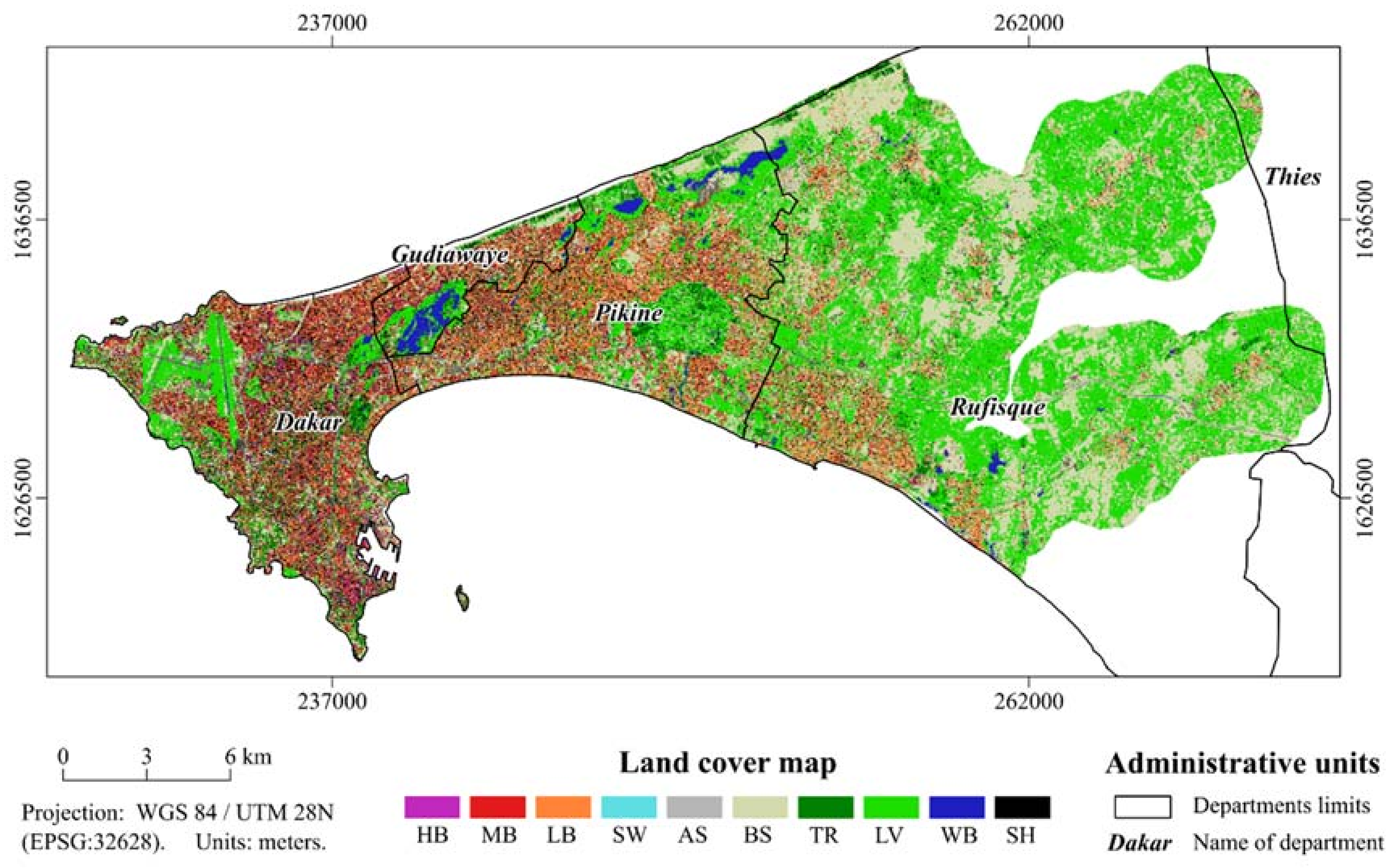
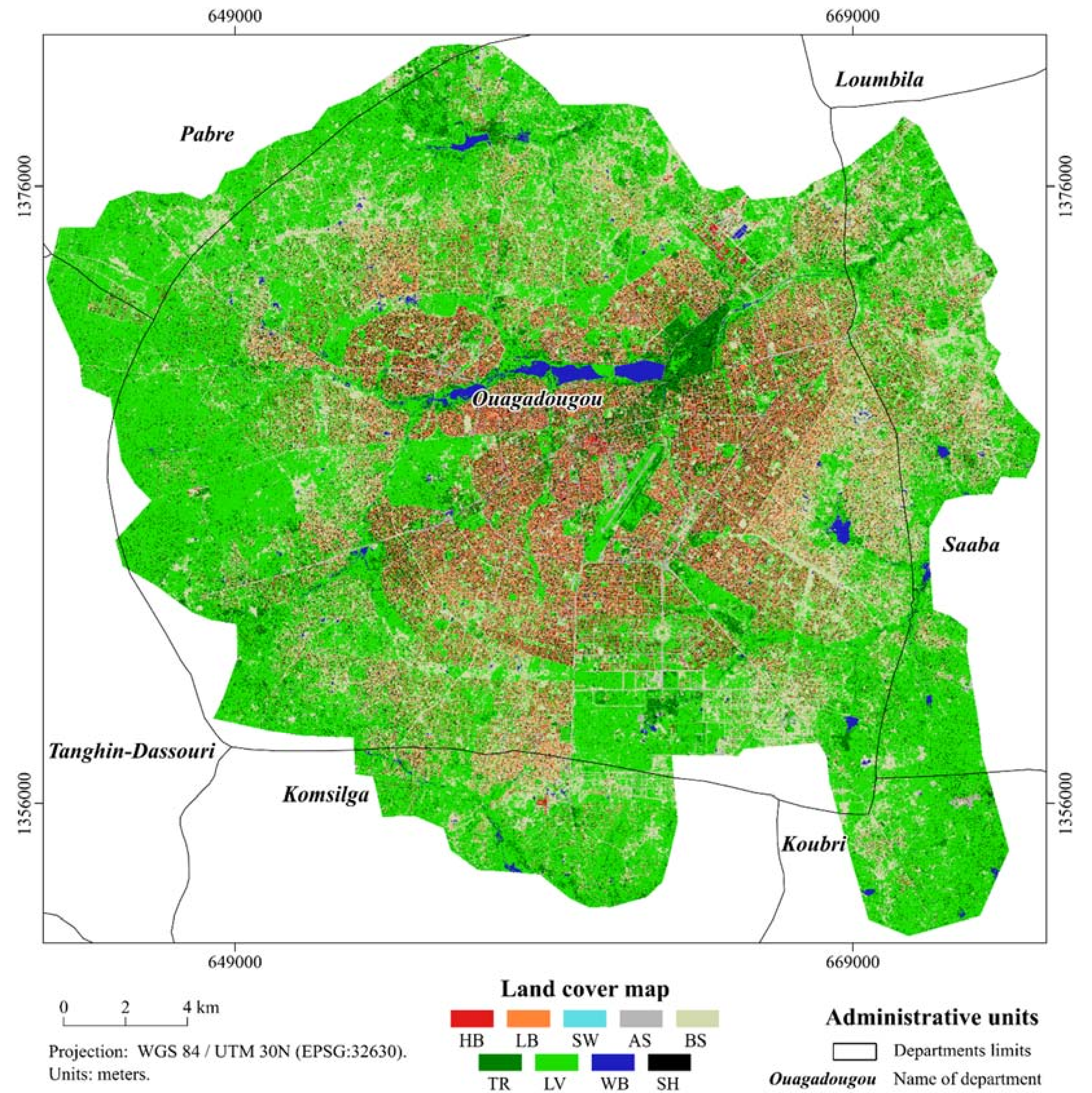
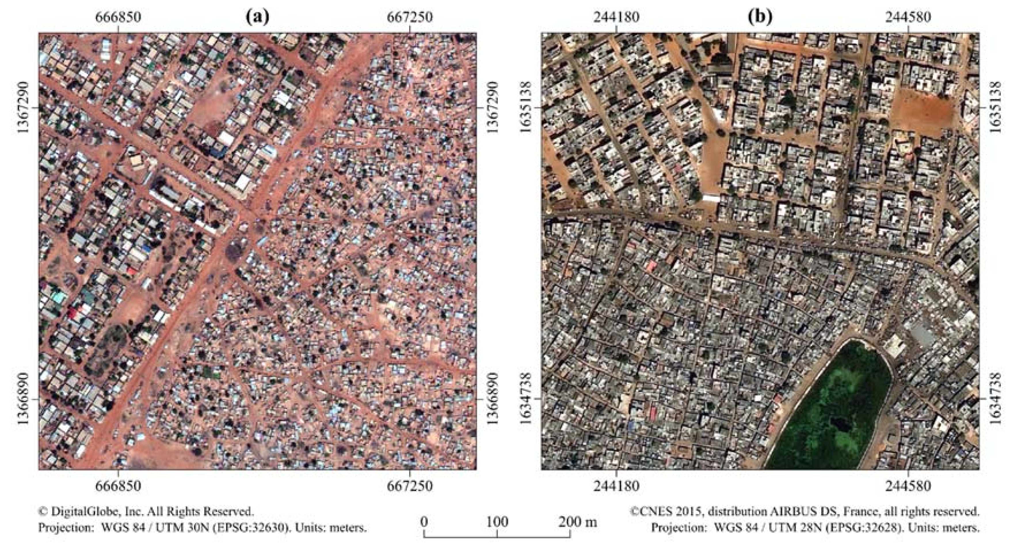
2.1. Study Areas

The methodology presented here was applied to two cities in Western Africa, namely Ouagadougou and Dakar, the capitals of Burkina Faso and Senegal, respectively. The areas of interests (AOI) were selected to cover both the core of the city and the peri-urban areas, as there is a lack of a well-established consensus for the definition and delineation of urban areas [32]. AOIs were selected through visual interpretation of VHR imagery and were not restricted to administrative units. This allowed for a wide capture of economic activities and urban sprawl. Figure 1 and Figure 2 illustrate the extents of the AOIs, covering 615 km² for Ouagadougou and 418 km² for Dakar, superimposed with the administrative units.

2.2. Input Data

The primary input data consisted of land-cover (LC) maps (Figure 1 and Figure 2) derived from very-high resolution (VHR) satellite imagery, i.e., WorldView-3 and Pléiades for Ouagadougou and Dakar, respectively, with a spatial resolution of 0.5 m. These were produced using a semiautomated object-based image analysis (OBIA) [33] framework based on open-source solutions [34,35,36,37]. The overall accuracy (OA) of the LC products was 93.4% and 89.5% for Ouagadougou and Dakar, respectively. Their legends are presented in

Table 1. Legend of the land-cover maps used as input to compute spatial metrics.

Ouagadougou—Burkina Faso		Dakar—Senegal
Class	Abbreviation	Class	Abbreviation
High buildings (>3 m)	HB	High buildings (>10 m)	HB
Low buildings (<3 m)	LB	Medium buildings (5–10 m)	MB
-	-	Low buildings (<5 m)	LB
Swimming pools	SW	Swimming pools	SW
Asphalt surfaces	AS	Artificial ground surfaces	AS
Bare soils	BS	Bare soils	BS
Trees	TR	Trees	TR
Low vegetation	LV	Low vegetation	LV
Water bodies	WB	Inland waters	WB
Shadows	SH	Shadows	SH

.

Additionally, normalized digital surface models (nDSM), i.e., datasets that contain the height of above-ground objects, were used. The nDSMs were derived from photogrammetric digital surface models (DSM) generated from a stereo triplet for Dakar and a stereo couple for Ouagadougou. Vegetation and water indices, i.e., normalized difference vegetation index (NDVI) and normalized difference water index (NDWI), respectively, were also used.

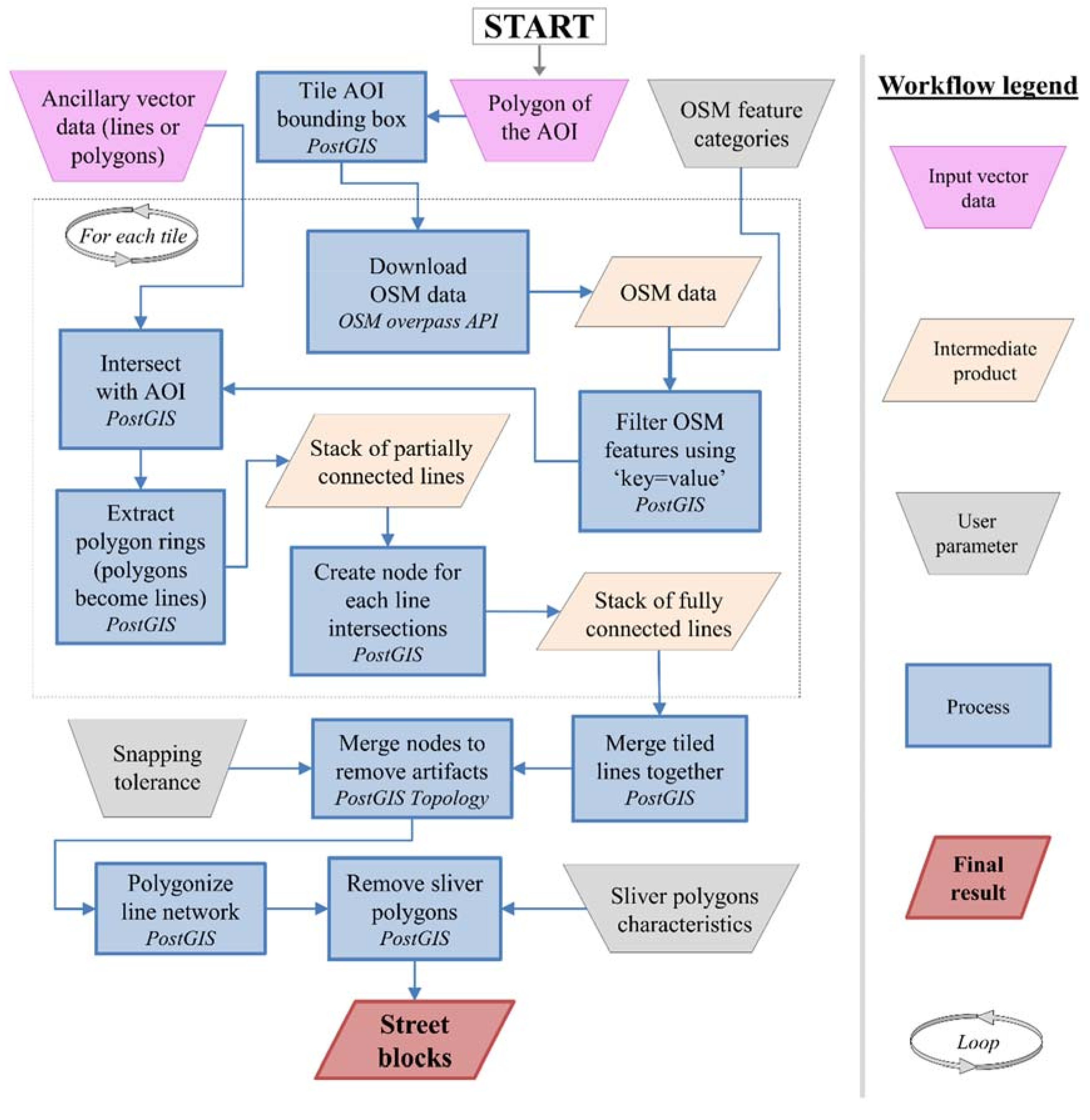
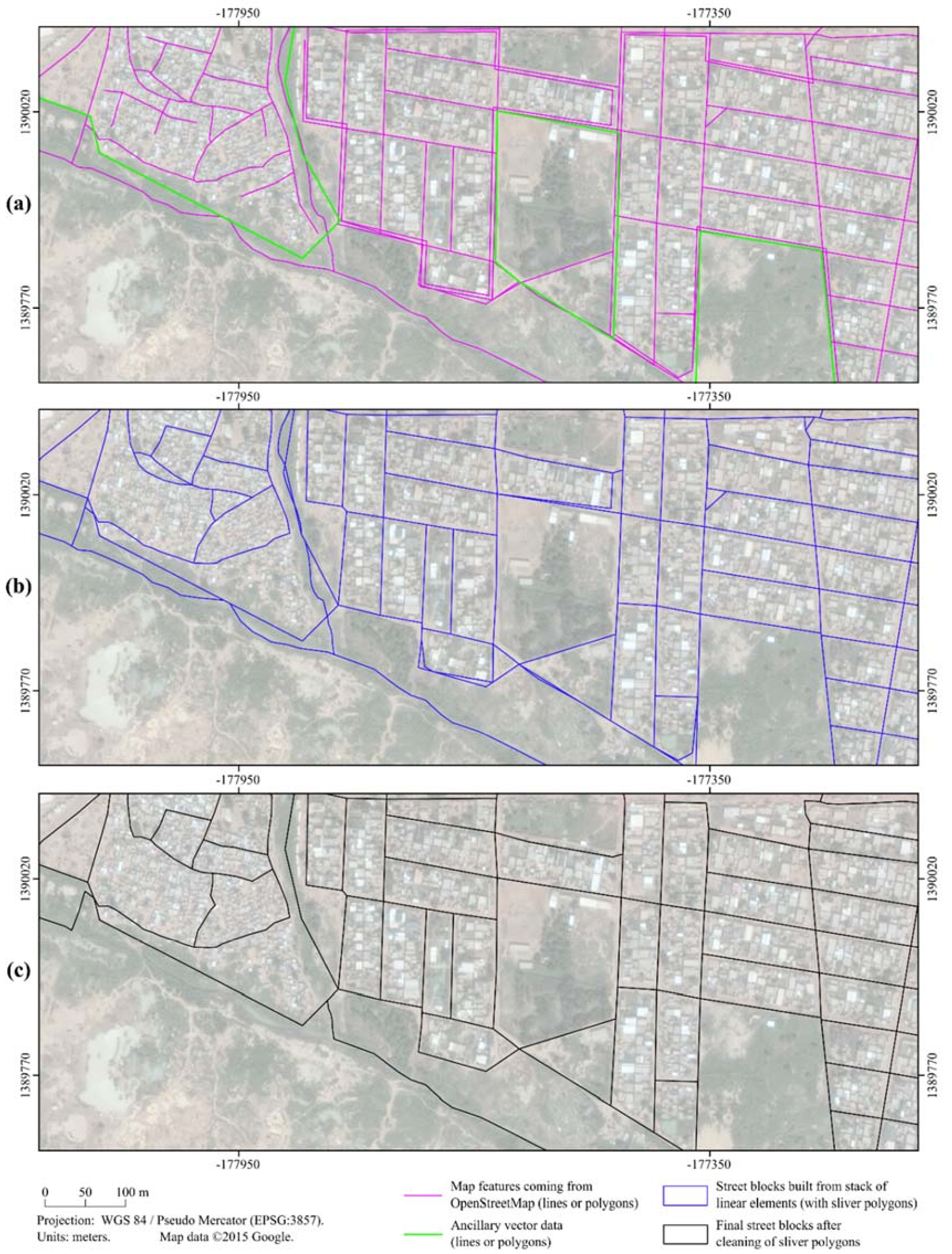
2.3. Extraction of Street Block Geometries Using OpenStreetMap

In OSM data, roads are the map features mostly associated with the highest completeness. A recent study [38] estimates that the OSM roads have reached more than 80% of completeness at a global scale. Although this high score hides important variations at regional or national scales, it encourages the use of this global dataset to develop solutions that can be applied worldwide.

In this research, we propose an approach similar to [19]. Our method is a semiautomated workflow exploiting the OpenStreetMap data for the creation of urban street blocks geometries, to be used as a fundamental urban landscape unit to map land use [16]. Different from proprietary solutions (ESRI ArcGIS) proposed in [19], it takes advantage of the open-source software PostGIS for storage, management, and processing of large vector datasets. The programming language is Python and the code is implemented in a “Jupyter notebook” [39] accessible under an open license on a dedicated online repository (Appendix B). It can be easily adapted to suit further research needs. The main steps are illustrated in Figure 3.

To map the land use at the street block level implies that blocks should have a high intrahomogeneity of the urban function. Indeed, it is important to get meaningful spatial units, according to the process investigated (here, the land use). Otherwise, the spatial metrics will be meaningless [40] and the classification task would be more complex, with more confusions between classes and lower confidence in the land-use maps produced.

The OSM road network alone could not adequately meet our needs. Indeed, in some situations, the edges of the blocks could be defined better using line segments of a river, hill, or other manmade structures [19]. Actual land use is often a mix of uses, and thus it is difficult to reach a situation where all street blocks extracted would be homogenous in terms of land use. However, incorporating other extra map features (e.g., rivers, water bodies, railways, military camps, cemeteries, residential areas, farmlands, etc.) allowed for these problems to be reduced. Consequently, the blocks that were produced were not street blocks stricto sensu, but they met the needs of our analysis. Moreover, vector data such as administrative city sectors or functional zones could be used as ancillary datasets in addition to OSM data.

The script starts by taking as input a polygon shapefile corresponding to the AOI and optionally some ancillary vector layers. Then, the bounding box of the AOI is created and subdivided into tiles and OSM data are automatically downloaded using the OSM extended overpass API [41]. Next, map features of interest are filtered according to their “key = value” pairs in the OSM tagging scheme [42,43]. The map features (i.e., lines and polygons) are then intersected with the extent of the AOI and the polygons are converted into linear features. At this point, some lines that cross each other without being connected, e.g., because they do not share a common node at their intersection, are processed to obtain a stack of fully connected lines. Owing to coregistration inaccuracies and/or nearly redundant road geometries in OSM [44] or between OSM and ancillary data, many sliver polygons are created. This is overcome by using the PostGIS topological functions to merge neighboring nodes according to a user-provided snapping tolerance. The snapping tolerance should not be too large because it is likely to distort the accurately digitized road sections and make further steps more difficult [44]. After this procedure, the street blocks polygons are extracted from the stack of lines. Similar to [19], two kinds of polygons are generated: (i) urban blocks and (ii) undesirable polygons (sliver polygons) resulting from multilane roads, functional roads near crossroads, or highway ramps. These sliver polygons are usually easily identifiable based on criteria of shape and size since they are thin and small. The user is here in charge of adapting the preset criteria to be used for identification of probable sliver polygons. The sliver polygons are then eliminated by merging them with their neighboring nonsliver polygon with which they shared the larger border. This latest step iterates until no sliver polygons remain, resulting in final block geometries.

2.4. Computing Street Block Features

In this research, street block features used to classify land use can be separated in two groups. The first relates to spatial metrics computed based on the land-cover maps available. The other group include additional information, such as block morphology or features derived directly from the spectral values. In total, 116 and 97 features were computed for Ouagadougou and Dakar, respectively. All metrics were computed in GRASS GIS, using an automated script coded in Python [45] which is available on a dedicated repository (see Appendix B).

2.4.1. Street Blocks’ Spatial Metrics (Patch-Based Metrics)

In this paper, the spatial metrics used are all related to the “patch mosaic” paradigm [40,46], whereby the landscape is viewed as a mosaic of land-cover patches. A patch could be defined as a group of neighboring pixels that belong to the same class. In that way, it acts as an abstraction level that masks some information of the actual landscape. For instance, in urban areas, a coalescence of hundreds of small individual buildings can form one single patch and could have the same size as a patch corresponding to a single large building, such as a commercial center. Amongst other things, this paradigm makes the use and interpretation of patch-based metrics difficult for nonexperts. According to [40], the behavior of spatial metrics are theoretically not well understood and their interpretation could be very challenging. There is a profusion of different patch-based metrics but all aiming at describing a landscape either on its composition/diversity or the spatial configuration of the patches it contains.

Different software can be used for computing spatial metrics and the best known is probably FRAGSTAT [23]. Unfortunately, its use is limited by the size of the dataset that can be handled [40] and offers limited automation. As an alternative, we used the “r.li” suite of modules, available in GRASS GIS [47]. These modules provide a set of landscape indices that can be found in FRAGSTATS and are designed not to overload the computer memory (i.e., the RAM), thus having the capacity to process large datasets [48]. Besides, GRASS GIS is built as a collection of hundreds small programs, enabling all common GIS operations to be handled in the same environment in a computationally efficient manner. Importantly, the process could be automated thanks to the Python application programming interface (API) [49]. The list of metrics computed is presented in

Table A1. Spatial metrics computed.

Level of Computation	Metric
Landscape level All land-cover classes together	Dominance
	Pielou
	Renyi
	Richness
	Shannon
	Simpson
Class level On binary maps (for each land-cover class separately)	Patch number
	Patch density
	Mean patch size
	SD of patch size
	Patch size coef. of variation
	Range of patch size
	Shape index
	Proportion

(see Appendix A).

2.4.2. Additional Street Block’s Features

In addition to the spatial metrics described above, features related to the shape of the street blocks were computed, as well as key features aggregated from spectral data, e.g., the median and standard deviation of NDVI and NDWI, for their ability in the characterization of nonbuilt landscapes. Those additional features were computed using “i.segment.stats” add-on of GRASS GIS [50]. Moreover, as information on the height of above-ground objects was available from the nDSMs, we computed the mean height of the building pixels.

Table A2. Additional block features computed.

Source of Information	Blocks Feature
Spectral	NDVI median
	NDVI mean
	NDWI median
	NDWI mean
nDSM models Built-up mask (from land-cover map)	Mean height of built pixels
	Number of built pixels
Block morphology (shape features)	Area
	Perimeter
	Compactness relative a to square
	Compactness relative a to circle
	Fractal dimension

(see Appendix A) summarizes the additional block features that are used in complement to spatial metrics.

2.5. Land Use Scheme and Sampling

The choice of the land-use classes constituting the legend scheme was made after a visual interpretation of the different types of urban structures and uses. Both cities are characterized by several types of land use such as industrial, commercial and services, administrative, or residential. In the land-use legend scheme (see

Table 2. Legend scheme of land use for Ouagadougou and Dakar and size of training and test sets (number of street block polygons).

Class	Abbreviation	Training Set Size	Test Set Size
Ouagadougou—Burkina Faso
Vegetation	VEG	122	41
Bare soils	BARE	173	57
Non-residential built-up (administrative, commercial, services, etc.)	ACS	220	68
Planned residential built-up	PLAN	268	83
Unplanned residential built-up	UNPLAN	302	90
Dakar—Senegal
Agricultural vegetation	AGRI	93	42
Natural vegetation	VEG	86	30
Bare soils	BARE	57	18
Non-residential built-up (administrative, commercial, services, etc.)	ACS	153	46
Planned residential built-up	PLAN	872	277
Deprived residential built-up	DEPR	209	68

), a clear focus is made on having a better thematic precision for residential areas than for other classes. It includes two residential classes enabling the distinction between planned (usually richer and with lower density) and unplanned/deprived (usually poorer and with higher density). The nonresidential built-up land uses, such as commercial, administrative, or services, were all grouped together in one single class. This was done because we intend to utilize the land-use information for further research regarding fine-scale modeling of population density.

Moreover, as we aimed at mapping the whole extent of the AOI, which encompasses peri-urban areas, we also included classes related to natural elements, e.g., vegetated or bare areas. Urban land use is often mixed because of the presence of multiple urban activities on the same block. However, our aim here was to map the dominant activity in the block. This explains the absence of “mixed” classes in the legends.

While urban patterns in Ouagadougou present a clear distinction between planned and unplanned neighborhoods (as visible in Figure 4a), in Dakar, the difference is less straightforward. There, some neighborhoods look more deprived than most of the residential areas, even if they present a semblance of regular street pattern (see Figure 4b). Previous research, integrating remote sensing and socioeconomic census data, proved that they are inhabited by a poorer population [51].

First, a set of 1648 and 1500 street blocks were randomly sampled for Dakar and Ouagadougou, respectively, for training a supervised classification algorithm and for validation. Each sampled block was then assigned a label by visual interpretation according to its supposed dominant land-use class. In the case of Dakar, the resulting training/test set was highly imbalanced, between “Planned residential” and “Deprived residential”. The same was true for “Agricultural vegetation” and “Natural vegetation”. For that reason, we manually sampled an extra 344 blocks to obtain a more balanced training/validation set. Next, for both case studies, a split in a 75%/25% ratio was made to get a training set and an independent validation set. During the process, the interpreter was asked about his confidence in giving an adequate label without any doubt. Finally, samples for which the interpretation decision was not certain, i.e., the experts were undecided about the land-use class to be attributed, were removed from the validation set (41 and 76 blocks removed for Dakar and Ouagadougou, respectively). This explains why the number of validation samples do not reach the 25% previously mentioned for some classes (see Table 1).

2.6. Feature Selection and Classification Using Machine Learning

A supervised random forest classifier (RF) was used for the classification step. RF is an ensemble of Classification and Regression Decision Trees (CARTs) [52], where each tree is trained on a random bootstrapped sample of the training data (about two-thirds of the data). In the end, a label is assigned, as derived from the combined predictions (majority voting) of each tree. Since RF is an aggregation of several individual and independent trees, it has been very commonly used in RS studies due to its high prediction accuracy and relative immunity to overfitting [53]. To maximize performance, two parameters are usually fine-tuned in RF, the number of trees to grow and the number of randomly selected features at each decision point (split) within a tree. The former is commonly suggested to be set as high as computationally efficient [52], while the value of the latter is identified through cross-validation of the out-of-sample training data, known as Out of Bag (OOB) error.

As already mentioned, many features were computed for both case studies. A large proportion were spatial metrics which are inherently highly correlated and redundant since they are all dependent on a small amount of basic patch metrics for their computation, e.g., area, perimeter, patch, and neighboring patch type [54]. This kind of dataset could result in an underperforming and unnecessarily complex classification model. Consequently, we performed a feature selection (FS) procedure prior to the classification step with the aim of constructing smaller, more predictive and parsimonious models [55]. The “Variable Selection Using Random Forest” (VSURF) algorithm, a popular automated method for FS selection developed by [56], was used. The salient features of VSURF are categorized in defining three types of feature subsets: (i) removing useless features, (ii) finding the most predictive set of features which may contain a great amount of redundancy, and (iii) retaining the accuracy while removing redundant features through a stepwise search.

Feature selection and classification were performed using the R software, version 3.5.0 [57]. The R code has been made available in R markdown format [58] on a dedicated repository (see Appendix B).

3. Results

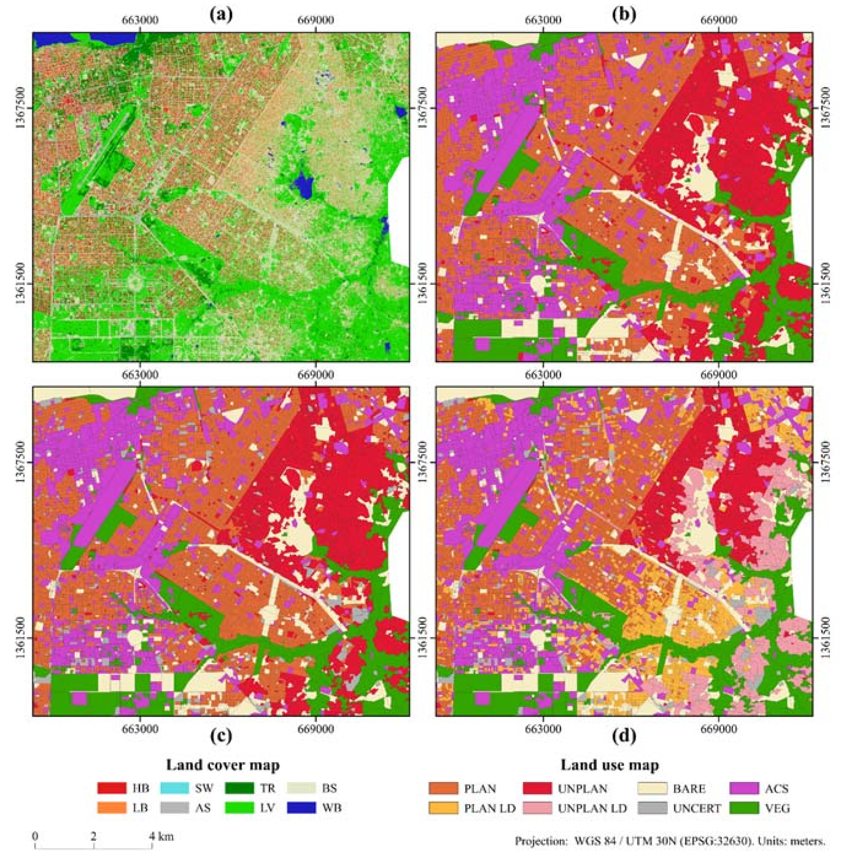
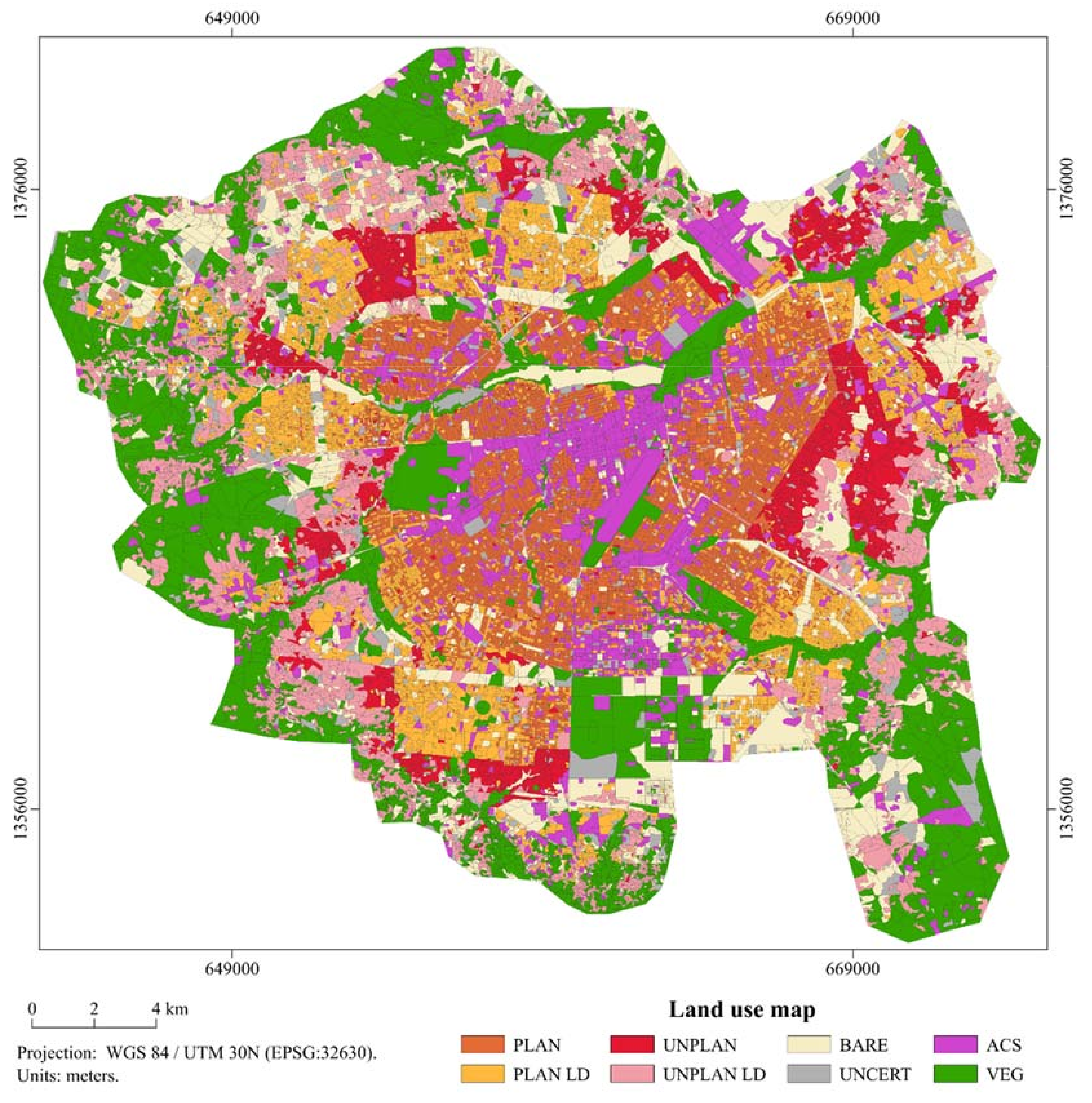
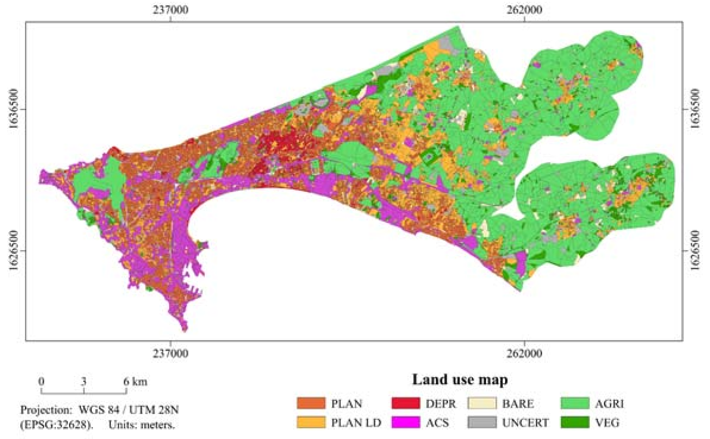
3.1. Extraction of Street Block Geometries

Our processing chain was used to create the street block geometries using a large amount of input data thanks to the capabilities of PostGIS. To give an order of magnitude, in Ouagadougou, more than 47,000 blocks were extracted from a set of more than 180,000 segments. The number of sliver polygons present after this initial extraction was quite impressive: 32.6% and 31.5% for Ouagadougou and Dakar, respectively. Sliver polygons were removed to produce a final layer containing nearly 32,000 street blocks geometries for Ouagadougou and 23,000 for Dakar. In Ouagadougou, an existing ancillary layer produced in a previous study [35], whereby the city had been delineated into local morphological zones, was used.

Figure 5 illustrates the results from different main steps of the processing chain. The initial stack of linear elements coming from OSM and ancillary data is quite chaotic (see Figure 5a). Snapping all nodes (here, with a snapping threshold of 7 m), enables efficient cleaning of the initial errors but some sliver polygons remain (see Figure 5b). The final geometries after the removal of sliver polygons are presented on Figure 5c.

3.2. Automated Feature Selection

Feature selection was performed on the initial set of features computed and resulted in an impressive reduction of 81.9% (from an initial set of 116 features to 21 remaining features) and 86.6% (from 97 initial features to 13 remaining) for Ouagadougou and Dakar, respectively. The list of selected features is presented in

Table 3. Blocks features selected by feature selection using “VSURF”. These are the remaining features at the “prediction” step.

	Case Studies
Street Block Features	Ouagadougou	Dakar
Landscape composition
Shannon	X	X
Dominance	X
Features relative to building class
High buildings mean patch size	X
SD of high buildings patch area	X
Proportion of high buildings pixels in the block	X
Proportion of medium buildings	NA	X
Proportion of low building pixels in the block	X	X
SD of low building patch area	X
Low building patch density	X	X
Low building patch number	X
Count of built pixels		X
Mean height of built pixels	X	X
Features relative to shadow class
Proportion of shadows pixels in the block		X
Shadows patch density	X	X
Shadows patch number	X
Features relative to other land-cover classes
Artificial surface shape index		X
Range of artificial surfaces patch area		X
SD of asphalt surface patch area	X
Bare soils patch density	X
Features relative to vegetation classes
Low vegetation patch density	X
Range of low vegetation patch area		X
Range of trees patch area	X
Trees mean patch size	X
Remote sensing indices
NDVI median	X	X
NDWI SD	X
Features relative to block morphology
Block perimeter		X
Compactness relative to a circle	X
Compactness relative to a square	X
Total	21	13

. Globally, spatial metrics relative to almost all land-cover classes are present in the set of selected features. However, it appears that classes related to different building heights are more represented, which is unsurprising. Moreover, features related to landscape composition, street block morphology, and remote sensing indices are also present, which proves their added-value in the classification model.

3.3. Land-Use Classification Using Random Forest

The reduced set of features was then used as an input dataset of a supervised classification using RF. The predictions of the model were evaluated using an independent validation set and overall accuracies of 84% and 79% were achieved for Ouagadougou and Dakar, respectively. However, these values hide disparities between classes. The F-score, e.g., a synthetic accuracy metric, is used here to compare the classification performance at the class level [59].

The class “Planned residential” performed similarly in both case studies with F-scores of 0.88 and 0.84 for Dakar and Ouagadougou, respectively. However, the class “Deprived residential”/“Unplanned residential” showed a strongly lower accuracy in Dakar, with an F-score of 0.68, while in Ouagadougou it was the best-performing class, reaching an impressive score of 0.92. The inspection of confusion matrices (

Table 4. Confusion matrix of land-use classification for Ouagadougou. VEG: Vegetation; BARE: Bare soils; ACS: Nonresidential built-up (administrative, commercial, services, etc.); PLAN: Planned residential; UNPLAN: Unplanned residential.

		Reference
	Classes	VEG	BARE	ACS	PLAN	UNPLAN
Prediction	VEG	36	7	0	0	2
	BARE	5	47	4	0	2
	ACS	0	0	47	7	0
	PLAN	0	2	14	79	2
	UNPLAN	0	1	3	4	77
	F-score	0.84	0.82	0.77	0.84	0.92

and

Table 5. Confusion matrix of land-use classification for Dakar. AGRI: Agricultural vegetation; VEG: Natural vegetation; BARE: Bare soils; ACS: Nonresidential built-up (administrative, commercial, services, etc.); PLAN: Planned residential; DEPR: Deprived residential.

		Reference
	Classes	AGRI	VEG	BARE	ACS	PLAN	DEPR
Prediction	AGRI	34	3	0	1	1	0
	VEG	6	17	2	4	3	0
	BARE	1	3	12	0	0	0
	ACS	1	4	1	24	8	1
	PLAN	0	3	2	15	253	25
	DEPR	0	0	1	1	12	42
	F-score	0.84	0.55	0.71	0.57	0.88	0.68

) revealed that while some confusions were present between the residential classes in Ouagadougou, they were of a larger magnitude in Dakar. In both cases, most of the confusion occurred between the “Plan residential” and “Nonresidential built-up” classes. Moreover, misclassifications appeared between “Bare soils” and “Low vegetation”, as was expected, since many nonbuilt street blocks present a mix of vegetated and bare soil elements.

The analysis of the RF feature importance reveals that, for both cases studies, the most important features are those related to the built environment (see

Table 6. Ouagadougou—Per class feature importance from the random forest classifier (mean decrease in accuracy). Only the 10 most important are presented. “SD” refers to standard deviation. The color-ramp indicates the feature importance for each land-use classes, with darker green corresponding to the top feature for each class (number in bold). ACS: Nonresidential built-up (administrative, commercial, services, etc.); BARE: Bare soils; PLAN: Planned residential; UNPLAN: Unplanned residential; VEG: Vegetation.

	Land Use Classes
Street Blocks Features	PLAN	UNPLAN	ACS	BARE	VEG	Overall
Mean height of built pixels	0.078	0.137	0.106	0.061	0.034	0.091
Proportion of high buildings patch	0.124	0.089	0.065	0.082	0.071	0.090
Low building patch density	0.085	0.120	0.024	0.045	0.165	0.084
Proportion of Low building patch	0.071	0.077	0.010	0.089	0.150	0.072
High buildings mean patch size	0.061	0.030	0.065	0.048	0.051	0.051
Low vegetation patch density	0.048	0.047	0.048	−0.004	0.032	0.038
NDVI median	0.006	0.030	0.007	0.015	0.257	0.042
Shadows patch density	0.024	0.087	0.018	0.076	−0.011	0.043
SD of high buildings patch area	0.039	0.047	0.055	0.042	0.043	0.045
Trees mean patch size	0.023	0.010	0.063	0.008	0.003	0.023

and

Table 7. Dakar—Per class feature importance from the random forest classifier (mean decrease in accuracy). Only the 10 most important are presented. The color-ramp indicates the feature importance for each land-use classes, with darker green corresponding to the top feature for each class (number in bold). ACS: Nonresidential built-up (administrative, commercial, services, etc.); AGRI: Agricultural vegetation; BARE: Bare soils; DEPR: Deprived residential; PLAN: Planned residential; VEG: Natural vegetation.

	Land Use Classes
Street Blocks Features	PLAN	DEPR	ACS	BARE	AGRI	VEG	Overall
Proportion of low buildings patch	0.070	0.164	0.017	0.100	0.259	0.122	0.098
Shadows patch density	0.080	0.055	0.032	0.039	0.047	0.097	0.069
Low buildings patch density	0.044	0.075	0.029	0.008	0.248	0.018	0.061
Mean height of built pixels	0.067	0.056	0.037	0.064	0.020	0.092	0.060
NDVI median	0.065	0.030	0.016	0.020	0.181	0.193	0.072
Proportion of shadows patch	0.050	0.095	0.004	0.051	0.080	0.066	0.055
Range of low vegetation patch area	0.024	0.016	−0.001	0.010	0.389	0.010	0.049
Count of built pixels	0.036	0.022	0.025	0.115	0.037	0.097	0.040
Range of artificial surfaces patch area	0.025	0.018	0.132	0.006	0.012	0.021	0.033
Proportion of medium buildings patch	0.065	0.002	0.002	0.025	0.088	0.013	0.047

). They are in the top-five features in Ouagadougou and in the top four in Dakar (assuming shadows are a proxy of the built-up patterns).

For the built-up classes, height is an important element, as witnessed by the selection of proportions of high and low buildings. It is interesting to notice the importance of shadows patch density as a top feature in Dakar for “Planned residential” which is not the case in Ouagadougou. This could be explained by the fact that residential buildings are more often multi-stories in Dakar than in Ouagadougou. Thereby, this shadow-related feature could be considered as a proxy of the presence of highly elevated built-up structures. Unsurprisingly, the vegetation index (NDVI) is the best feature for the vegetated land-use classes. Bare soils also present a feature related to the built land-cover classes. We assume it should be an inverse relation, i.e., characterizing the blocks as having no presence of built-up.

3.4. Introduction of Uncertainty and Thematic Improvement of Final Products

Errors and uncertainty are inherent in any classification problem. Even if the classifier provides a class label for each item, predictions could be affected by a high level of uncertainty. RF natively provides the class probability for each street block [60]. We take the decision to use this essential information to reclassify street blocks for which the prediction was highly uncertain. We compute the difference between the probabilities of the most probable and the second most probable class. Street blocks having a difference of less than 5 percentage points were then relabeled as “Uncertain” (see Figure 6c). It concerns 3.7% and 4.1% of the available street blocks for Ouagadougou and Dakar, respectively. For the convenience of the users, all class probabilities are included in the product releases.

Residential built-up density is usually a good indicator of population densities. For that reason, we use the information about blocks’ percentage of built-up patches to discriminate between different densities of built-up. (Figure 6d). In both case studies, street blocks classified as “Planned residential” were relabeled as “Planned residential (low density)” if their built-up percentage was lower than 30% and 40% for Ouagadougou and Dakar, respectively. In Ouagadougou, the same approach was used to distinguish two classes of built-up density for the “Unplanned residential” class, with a threshold fixed at 15% of built-up, and to enable a split between peri-urban settlements and slum-like patterns. The choice of these thresholds was made through trial-and-error, relying on visual assessment of the land-cover map. The final land-use maps are visible in Figure 7 and Figure 8. For the convenience of the reader, they can be visualized online along with the land-cover information (https://tgrippa.github.io/Landuse_from_landcover_webmap/).

4. Discussion

The solution proposed in this paper proved to be operational for processing very large areas, as our case studies datasets cover more than 1000 km² in total, with a spatial resolution of 0.5 m. However, some limitations can be highlighted.

The first limitation relates to the completeness of OSM data. A quantitative evaluation of the geometric and semantic quality of the street blocks is out of the scope of this article, but some aspects can be discussed. A qualitative visual assessment shows that the consistency is more evident in the core urban areas, where the street network is denser and OSM data generally more complete. From several tests that were carried out, we concluded that the resulting street blocks may not be as detailed as expected, e.g., presence of polygons that are too large and encompass multiple distinct land uses. This is mostly related to the fact that the OSM database is not complete enough for certain locations, especially in peri-urban areas. To solve this issue, time was dedicated to the digitization of additional map features in OSM (e.g., roads, tracks, natural elements, etc.) at the periphery of our AOIs (peri-urban areas) to meet our requirements. This also contributed to the completion of the OSM database, which is a positive outcome. Since the OSM data completeness is increasing, it is likely that such issues will become less prevalent in the future. However, the performance of the proposed framework is likely to decrease as the landscape becomes more rural. Further research could look for other strategies for the automated extraction of meaningful landscape units for mapping the land use in rural and peri-urban areas.

The second limitation is linked to the spatial metrics. The selection of relevant spatial metrics for the phenomenon under investigation and the interpretation of their behaviors can be a challenging task in itself [40]. Moreover, it is likely that some metrics that perform well in one case study are less discriminant for another. It was the case in our results and this could be interpreted because of differences in terms of urban landscapes. As a solution, computing many metrics and feeding them into a feature selection procedure allows for the unsupervised selection of a parsimonious set of features.

Thirdly, the labelling procedure for creating the training and validation sets may clearly be a bottleneck if automation is mandatory. Further research could explore the possibility of taking advantage of the OSM database for the automatic selection and labeling of these samples, as OSM contains some information on land use and Point of Interest (POI).

Next, future studies aiming at implementing the same kind of workflow that we present here should consider the possibility of improving efficiency by computing the metrics for the street blocks belonging to the training samples only. Since they are sufficient for performing the feature selection step, this would save processing time and storage space [61]. Only the most discriminant features could then be computed for the whole AOI. This approach would allow for computing a very large number of features without creating computational and storage issues.

Finally, as previously mentioned (see Section 2.4.1), the “patch mosaic” paradigm hides some aspects of the urban structures, which is likely to limit the ability of spatial metrics to adequately characterize urban land use. Possible future work should investigate a broader workflow that would include explicit information derived from the OBIA segmentation process. For example, information on individual segments could be computed, e.g., area, compactness, and fractal dimension, and then summarized either at the class or at the landscape level.

Prediction errors and the corollary uncertainty of the produced maps are important points that any classification framework should consider. In this study, we used the class-probability output from the RF model to identify street blocks for which the prediction was affected by an important level of uncertainty. In addition to the land-use maps where labels correspond to the most probable class, we also provide the class-probability values for each street block. This information is useful especially when classification products are used as input data to other classification or modeling tasks since it is well known that errors propagate to the derived products. In the future, we plan to carry out sensitivity analysis to assess how errors and uncertainty of land-cover maps affect the derived land use and the models of spatial distribution of population densities.

5. Conclusions

While availability of up-to-date and reliable geographical information on urban areas is sorely missing in developing countries, new sources of information such as VGI can overcome existing challenges. This research presented a workflow, mostly automated, for mapping urban land use at the street block level, with a focus on residential use. The proposed framework proved its ability to efficiently handle large datasets, since the two case studies, Ouagadougou and Dakar, covering more than 1000 km² in total, achieved 84% and 79%, respectively. All of the computer codes developed and the resulting datasets have been released in open-access to any interested users.

References

1. UN DESA. World Urbanization Prospects: The 2018 Revision, Online ed; United nations, Department of Economic and Social Affairs: New York, NY, USA, 2018. [Google Scholar]
2. Novack, T.; Kux, H.; Feitosa, R.; Costa, G. Per block urban land use interpretation using optical VHR data and the knowledge-based system Interimage. Int. Arch. Photogramm. Remote Sens. Spat. Inf. Sci. 2010, 38, 6. [Google Scholar]
3. Mennecke, B.E.; West, L.A., Jr. Geographic Information Systems in Developing Countries: Issues in Data Collection, Implementation and Management. J. Glob. Inf. Manag. 2001, 9, 44–54. [Google Scholar] [CrossRef]
4. Eria, S. The State of GIS in Developing Countries: A Diffusion and GIS & Society Analysis of Uganda, and the Potential for Mobile Location-Based Services. Ph.D. Thesis, University of Minnesota, Minneapolis, MN, USA, 2012. [Google Scholar]
5. Tumba, A.G.; Ahmad, A. Geographic information system and spatial data infrastructure: A developing societies’ perception. Univers. J. Geosci. 2014, 2, 85–92. [Google Scholar] [CrossRef]
6. Schwabe, C.A. The geoinformation industry in Africa: Prospects and potentials. In Proceedings of the Fourth Meeting of the Committee on Development Information (CODI IV), Addis Ababa, Ethiopia, 23–28 April 2005. [Google Scholar]
7. Schwabe, C. Getting Geoinformation and SDI to Work for Africa–Part 2; PositionIT: Gauteng, South Africa, 2010. [Google Scholar]
8. Economic Commission for Africa, United Nations. Geospatial Information for Sustainable Development in Africa: African Action Plan on Global Geospatial Information Management; Economic Commission for Africa, United Nations: Addis Ababa, Ethiopia, 2017. [Google Scholar]
9. Goodchild, M.F. Citizens as sensors: The world of volunteered geography. GeoJournal 2007, 69, 211–221. [Google Scholar] [CrossRef]
10. Walde, I.; Hese, S.; Berger, C.; Schmullius, C. From land cover-graphs to urban structure types. Int. J. Geogr. Inf. Sci. 2014, 28, 584–609. [Google Scholar] [CrossRef]
11. Vanderhaegen, S.; Canters, F. Mapping urban form and function at city block level using spatial metrics. Landsc. Urban Plan. 2017, 167, 399–409. [Google Scholar] [CrossRef]
12. Voltersen, M.; Berger, C.; Hese, S.; Schmullius, C. Object-based land cover mapping and comprehensive feature calculation for an automated derivation of urban structure types at block level. Remote Sens. Environ. 2014, 154, 192–201. [Google Scholar] [CrossRef]
13. Siksna, A. The effects of block size and form in North American and Australian city centres. Urban Morphol. 1997, 1, 19–33. [Google Scholar]
14. Almeida, C.M.D.; Monteiro, A.M.V.; Câmara, G.; Soares-Filho, B.S.; Cerqueira, G.C.; Pennachin, C.L.; Batty, M. GIS and remote sensing as tools for the simulation of urban land-use change. Int. J. Remote Sens. 2005, 26, 759–774. [Google Scholar] [CrossRef]
15. Bochow, M.; Taubenbock, H.; Segl, K.; Kaufmann, H. An automated and adaptable approach for characterizing and partitioning cities into urban structure types. In Proceedings of the 2010 IEEE International Geoscience and Remote Sensing Symposium, Honolulu, HI, USA, 25–30 July 2010; pp. 1796–1799. [Google Scholar] [CrossRef]
16. Grippa, T. Osm Street Blocks Extraction (Version V1.0). Zenodo 2018. [Google Scholar] [CrossRef]
17. Fonte, C.; Minghini, M.; Patriarca, J.; Antoniou, V.; See, L.; Skopeliti, A. Generating Up-to-Date and Detailed Land Use and Land Cover Maps Using OpenStreetMap and GlobeLand30. ISPRS Int. J. Geo-Inf. 2017, 6, 125. [Google Scholar] [CrossRef]
18. Long, Y.; Liu, X. Automated identification and characterization of parcels (AICP) with OpenStreetMap and Points of Interest. Environ. Plan. B Plan. Des. 2016, 43, 341–360. [Google Scholar]
19. Fan, H.; Yang, B.; Zipf, A.; Rousell, A. A polygon-based approach for matching OpenStreetMap road networks with regional transit authority data. Int. J. Geogr. Inf. Sci. 2016, 30, 748–764. [Google Scholar] [CrossRef]
20. Simwanda, M.; Murayama, Y. Integrating Geospatial Techniques for Urban Land Use Classification in the Developing Sub-Saharan African City of Lusaka, Zambia. ISPRS Int. J. Geo-Inf. 2017, 6, 102. [Google Scholar] [CrossRef]
21. Hu, T.; Yang, J.; Li, X.; Gong, P. Mapping Urban Land Use by Using Landsat Images and Open Social Data. Remote Sens. 2016, 8, 151. [Google Scholar] [CrossRef]
22. Aubrecht, C.; Steinnocher, K.; Hollaus, M.; Wagner, W. Integrating earth observation and GIScience for high resolution spatial and functional modeling of urban land use. Comput. Environ. Urban Syst. 2009, 33, 15–25. [Google Scholar] [CrossRef]
23. McGarigal, K.; Marks, B.J. FRAGSTATS: Spatial Pattern Analysis Program for Quantifying Landscape Structure; U.S. Department of Agriculture, Forest Service, Pacific Northwest Research Station: Portland, OR, USA, 1995. [Google Scholar]
24. Turner, M.G.; Gardner, R.H. Landscape Ecology in Theory and Practice; Springer: New York, NY, USA, 2015; ISBN 978-1-4939-2793-7. [Google Scholar]
25. Urban, D.L.; O’Neill, R.V.; Shugart, H.H. Landscape Ecology. BioScience 1987, 37, 119–127. [Google Scholar] [CrossRef]
26. Uuemaa, E.; Mander, Ü.; Marja, R. Trends in the use of landscape spatial metrics as landscape indicators: A review. Ecol. Indic. 2013, 28, 100–106. [Google Scholar] [CrossRef]
27. Lowry, J.H.; Lowry, M.B. Comparing spatial metrics that quantify urban form. Comput. Environ. Urban Syst. 2014, 44, 59–67. [Google Scholar] [CrossRef]
28. Luck, M.; Wu, J. A gradient analysis of urban landscape pattern: A case study from the Phoenix metropolitan region, Arizona, USA. Landsc. Ecol. 2002, 17, 327–339. [Google Scholar] [CrossRef]
29. Herold, M.; Scepan, J.; Clarke, K.C. The use of remote sensing and landscape metrics to describe structures and changes in urban land uses. Environ. Plan. A 2002, 34, 1443–1458. [Google Scholar] [CrossRef]
30. Petrov, A. One Hundred Years of Dasymetric Mapping: Back to the Origin. Cartogr. J. 2012, 49, 256–264. [Google Scholar] [CrossRef]
31. Mennis, J. Generating Surface Models of Population Using Dasymetric Mapping. Prof. Geogr. 2003, 55, 31–42. [Google Scholar] [CrossRef]
32. Gisbert, F.J.G.; Martí, I.C.; Gielen, E. Clustering cities through urban metrics analysis. J. Urban Des. 2017, 22, 689–708. [Google Scholar] [CrossRef]
33. Blaschke, T.; Hay, G.J.; Kelly, M.; Lang, S.; Hofmann, P.; Addink, E.; Queiroz Feitosa, R.; van der Meer, F.; van der Werff, H.; van Coillie, F.; et al. Geographic Object-Based Image Analysis—Towards a new paradigm. ISPRS J. Photogramm. Remote Sens. 2014, 87, 180–191. [Google Scholar] [CrossRef] [PubMed]
34. Grippa, T.; Lennert, M.; Beaumont, B.; Vanhuysse, S.; Stephenne, N.; Wolff, E. An Open-Source Semi-Automated Processing Chain for Urban Object-Based Classification. Remote Sens. 2017, 9, 358. [Google Scholar] [CrossRef]
35. Grippa, T.; Georganos, S.; Vanhuysse, S.G.; Lennert, M.; Wolff, E. A local segmentation parameter optimization approach for mapping heterogeneous urban environments using VHR imagery. In Proceedings of the Remote Sensing Technologies and Applications in Urban Environments II, Warsaw, Poland, 4 October 2017; Volume 10431. [Google Scholar] [CrossRef]
36. Georganos, S.; Grippa, T.; Lennert, M.; Vanhuysse, S.; Wolff, E. SPUSPO: Spatially Partitioned Unsupervised Segmentation Parameter Optimization for efficiently segmenting large heterogeneous areas. In Proceedings of the 2017 Conference on Big Data from Space (BiDS’17), Toulouse, France, 28–30 November 2017. [Google Scholar]
37. Vanhuysse, S.; Grippa, T.; Lennert, M.; Wolff, E.; Idrissa, M. Contribution of nDSM derived from VHR stereo imagery to urban land-cover mapping in Sub-Saharan Africa. In Proceedings of the 2017 Joint Urban Remote Sensing Event (JURSE), Dubai, UAE, 6–8 March 2017. [Google Scholar]
38. Barrington-Leigh, C.; Millard-Ball, A. The world’s user-generated road map is more than 80% complete. PLoS ONE 2017, 12, e0180698. [Google Scholar] [CrossRef] [PubMed]
39. Kluyver, T.; Ragan-Kelley, B.; Pérez, F.; Granger, B.; Bussonnier, M.; Frederic, J.; Kelley, K.; Hamrick, J.; Grout, J.; Corlay, S.; et al. Jupyter Notebooks—A publishing format for reproducible computational workflows. In Proceedings of the 20th International Conference on Electronic Publishing; Göttingen, Germany, 7–9 June 2016; pp. 87–87. [Google Scholar] [CrossRef]
40. McGarigal, K. FRAGSTATS help v.4.2 2015. Available online: https://www.umass.edu/landeco/research/fragstats/documents/fragstats.help.4.2.pdf (accessed on 1 June 2018).
41. OpenStreetMap Wiki contributors Overpass API—OpenStreetMap Wiki. 2018. Available online: https://wiki.openstreetmap.org/wiki/Overpass_API (accessed on 1 June 2018).
42. Davidovic, N.; Mooney, P.; Stoimenov, L.; Minghini, M. Tagging in Volunteered Geographic Information: An Analysis of Tagging Practices for Cities and Urban Regions in OpenStreetMap. ISPRS Int. J. Geo-Inf. 2016, 5, 232. [Google Scholar] [CrossRef]
43. Vandecasteele, A.; Devillers, R. Improving Volunteered Geographic Information Quality Using a Tag Recommender System: The Case of OpenStreetMap. In OpenStreetMap in GIScience; Arsanjani, J.J., Zipf, A., Mooney, P., Helbich, M., Eds.; Lecture Notes in Geoinformation and Cartography; Springer: Basel, Switzerland, 2015; pp. 59–80. ISBN 978-3-319-14279-1. [Google Scholar]
44. Li, Q.; Fan, H.; Luan, X.; Yang, B.; Liu, L. Polygon-based approach for extracting multilane roads from OpenStreetMap urban road networks. Int. J. Geogr. Inf. Sci. 2014, 28, 2200–2219. [Google Scholar] [CrossRef]
45. Grippa, T. Street Blocks Features Computation (Version V1.0). Zenodo 2018. [Google Scholar] [CrossRef]
46. McGarigal, K.; Tagil, S.; Cushman, S.A. Surface metrics: An alternative to patch metrics for the quantification of landscape structure. Landsc. Ecol. 2009, 24, 433–450. [Google Scholar] [CrossRef]
47. Porta, C.; Spano, L.D.; Metz, M.; GRASS Development Team. Module r.li.*. 2017. Available online: https://grass.osgeo.org/grass74/manuals/r.li.html (accessed on 1 June 2018).
48. Neteler, M.; Mitasova, H. Open Source GIS—A GRASS GIS Approach; Springer: New York, NY, UISA, 2008. [Google Scholar]
49. Neteler, M.; Beaudette, D.E.; Cavallini, P.; Lami, L.; Cepicky, J. Grass gis. In Open Source Approaches in Spatial Data Handling; Springer: Berlin/Heidelberg, Germany, 2008; pp. 171–199. ISBN 978-3-540-74831-1. [Google Scholar]
50. Lennert, M.; GRASS Development Team. Addon i.segment.stats. Geographic Resources Analysis Support System (GRASS) Software, Version 7.3.; Open Source Geospatial Foundation: Chicago, IL, USA, 2016. [Google Scholar]
51. Borderon, M.; Oliveau, S.; Machault, V.; Vignolles, C.; Lacaux, J.-P.; N’Donky, A. Qualifier les espaces urbains à Dakar, Sénégal. Cybergeo Eur. J. Geogr. 2014. [Google Scholar] [CrossRef]
52. Breiman, L. Random forests. Mach. Learn. 2001, 45, 5–32. [Google Scholar] [CrossRef]
53. Belgiu, M.; Drăgut, L. Random forest in remote sensing: A review of applications and future directions. ISPRS J. Photogramm. Remote Sens. 2016, 114, 24–31. [Google Scholar] [CrossRef]
54. Cushman, S.A.; McGarigal, K.; Neel, M.C. Parsimony in landscape metrics: Strength, universality, and consistency. Ecol. Indic. 2008, 8, 691–703. [Google Scholar] [CrossRef]
55. Guyon, I.; Elisseeff, A. An introduction to variable and feature selection. J. Mach. Learn. Res. 2003, 3, 1157–1182. [Google Scholar]
56. Genuer, R.; Poggi, J.-M.; Tuleau-Malot, C. VSURF: An R Package for Variable Selection Using Random Forests. R J. 2015, 7, 19–33. [Google Scholar]
57. R Development Core Team. R: A Language and Environment for Statistical Computing; Version 3.5.0; R Foundation for Statistical Computing: Vienna, Austria, 2008; ISBN 3-900051-07-0. [Google Scholar]
58. Baumer, B.; Cetinkaya-Rundel, M.; Bray, A.; Loi, L.; Horton, N.J. R Markdown: Integrating a reproducible analysis tool into introductory statistics. arXiv, 2014; arXiv:1402.1894. [Google Scholar]
59. Sokolova, M.; Lapalme, G. A systematic analysis of performance measures for classification tasks. Inf. Process. Manag. 2009, 45, 427–437. [Google Scholar] [CrossRef]
60. Chunyang, L. Probability Estimation in Random Forests. Master’s Thesis, Department of Mathematics and Statistics, Utah State University, Logan, UT, USA, 2013. [Google Scholar]
61. Georganos, S.; Grippa, T.; Vanhuysse, S.; Lennert, M.; Shimoni, M.; Kalogirou, S.; Wolff, E. Less is more: Optimizing classification performance through feature selection in a very-high-resolution remote sensing object-based urban application. GISci. Remote Sens. 2017, 1. [Google Scholar] [CrossRef]
62. Grippa, T.; Georganos, S. Ouagadougou Very-High Resolution Land Cover Map (Version V1.0) [Data set]. Zenodo 2018. [Google Scholar] [CrossRef]
63. Grippa, T.; Georganos, S. Dakar Very-High Resolution Land Cover Map (Version V1.0) [Data set]. Zenodo 2018. [Google Scholar] [CrossRef]
64. Grippa, T.; Georganos, S. Ouagadougou Land Use Map at Street Block Level (Version V1.0) [Data set]. Zenodo 2018. [Google Scholar] [CrossRef]
65. Grippa, T.; Georganos, S. Dakar Land Use Map at Street Block Level (Version V1.0) [Data set]. Zenodo 2018. [Google Scholar] [CrossRef]
Figure 1. Land-cover map of Dakar superimposed with administrative units. HB: High buildings; MB: Medium buildings; LB: Low buildings; SW: Swimming pools; AS: Asphalt surfaces; BS: Bare soils; TR: Trees; LV: Low vegetation; WB: Water bodies; SH: Shadows.
Ijgi 07 00246 g001
Figure 2. Land-cover map of Ouagadougou superimposed with administrative units. HB: High buildings; LB: Low buildings; SW: Swimming pools; AS: Asphalt surfaces; BS: Bare soils; TR: Trees; LV: Low vegetation; WB: Water bodies; SH: Shadows.
Ijgi 07 00246 g002
Figure 3. Flowchart of the semiautomated processing chain for the extraction of street blocks from OpenStreetMap and ancillary vector data.
Ijgi 07 00246 g003
Figure 4. (a) Opposition between planned residential neighborhoods and unplanned ones in Ouagadougou. (b) Opposition between planned residential areas and deprived (poorer) neighborhoods in Dakar.
Ijgi 07 00246 g004
Figure 5. Extraction of street blocks from OSM data and ancillary vector data. (a) Lines and polygons coming from OSM and ancillary vector layer; (b) Street blocks that contain several undesired polygons (sliver polygons); (c) Final street blocks extracted.
Ijgi 07 00246 g005
Figure 6. Addition of uncertainty and built-up density to refine the thematic precision of the maps for Ouagadougou. (a) Land cover map for comparison purpose; (b) Most probable class from the random forest classifier; (c) Introducing “Uncertain” class; (d) Thematic refinement of residential classes according to the computed proportion of buildings. Land-cover classes (a) HB: High buildings; LB: Low buildings; SW: Swimming pools; AS: Asphalt surfaces; BS: Bare soils; TR: Trees; LV: Low vegetation; WB: Water bodies; SH: Shadows. Land-use classes (bd) VEG: Vegetation; BARE: Bare soils; ACS: Nonresidential built-up (administrative, commercial, services, etc.); PLAN: Planned residential; PLAN LD: Planned residential (low density); UNPLAN: Unplanned residential; UNPLAN LD: Unplanned residential (lox density); UNCERT: Uncertain prediction.
Ijgi 07 00246 g006
Figure 7. Land-use map of Dakar. AGRI: Agricultural vegetation; VEG: Natural vegetation; BARE: Bare soils; ACS: Nonresidential built-up (administrative, commercial, services, etc.); PLAN: Planned residential; PLAN LD: Planned residential (low density); DEPR: Deprived residential; UNCERT: Uncertain prediction.
Ijgi 07 00246 g007
Figure 8. Land-use map of Ouagadougou. VEG: Vegetation; BARE: Bare soils; ACS: Nonresidential built-up (administrative, commercial, services, etc.); PLAN: Planned residential; PLAN LD: Planned residential (low density); UNPLAN: Unplanned residential; UNPLAN LD: Unplanned residential (lox density); UNCERT: Uncertain prediction.
Ijgi 07 00246 g008