Multitemporal SAR Data and 2D Hydrodynamic Model Flood Scenario Dynamics Assessment

Abstract

The increasing number of floods and the severity of their consequences, which is caused by phenomena, such as climate change and uncontrolled urbanization, create a growing need to develop operational procedures and tools for accurate and timely flood mapping and management. Synthetic Aperture Radar (SAR), with its day, night, and cloud-penetrating capacity, has proven to be a very useful source of information during calibration of hydrodynamic models considered indispensable tools for near real-time flood forecasting and monitoring. The paper begins with the analysis of radar signatures of temporal series of SAR data, by exploiting the short revisit time of the images that are provided by the Cosmo-SkyMed constellation of four satellites, in combination with a Digital Elevation Model for the extraction of flood extent and spatially distributed water depth in a flat area with complex topography during a flood event. These SAR-based hazard maps were then used to perform a bi-dimensional hydraulic model calibration on the November 2010 flood event at the mouth of the Bradano River in Basilicata, Italy. Once the best fit between flood predictions of hydrodynamic models was identified and the efficacy of SAR data in correcting hydrodynamic inconsistencies with regard to reliable assessment of flood extent and water-depth maps was shown by validation with the December 2013 Bradano River event. Based on calibration and validation results, the paper aims to show how the combination of the time series of Synthetic Aperture Radar (SAR) and Digital Elevation Model (DEM) derived water-depth maps with the data from the hydrodynamic model can provide valuable information for flood dynamics monitoring in a flat area with complex topography. Future research should focus on the integration and implementation of the semi-automatic proposed method in an operational system for near real-time flood management.

1. Introduction

Floods are one of the most frequently occurring and costliest hazards worldwide. Between 1998 and 2009 alone, the European Environment Agency estimated that 213 flood events in Europe caused about 1126 fatalities, affected more than 3 million people, and caused at least 52 billion in losses [1]. Moreover, the United Nation [2] has estimated that one third of the world’s population (around 2.3 billion people) has been affected by floods in the last 20 years.

The expectation that large-scale flood damage will increase over time due to climate and land-use change and social growth in flood-prone areas has raised public and policymaker awareness with regard to operationalization of procedures and actions that will reduce flood effects and increase urban resilience [3].

Since budgets for risk management are limited, the choice of appropriate measurements (structural and non-structural), the assessment of the costs and effects of such measurements, and their prioritization are crucial for decision makers [4], who must keep overall spending to a minimum for all stages of the flood risk management cycle (i.e., risk analysis and reduction, emergency response, recovery, and reconstruction [5]). In this context, accurate prior damage evaluation has emerged as a necessity for the cost-effective risk reduction actions ([6,7]). Moreover, prompt assessment of damage in the early-recovery response phase is becoming decisive for coping with residual risk, in particular, for rescue organization and relief efforts ([8,9]).

In this context, during the monitoring and relief stages of a disaster risk reduction (DRR) cycle, an accurate representation is required of the flood event in terms of spatio-temporal dynamics and with regard to forecasting consequences [10]. Despite active research in this technical and research field, the combination of the complex and chaotic nature of flooding, the (often) fast dynamics of the phenomenon, and the increasing need for on-demand, in situ high spatial resolution data make particularly complicated to perform rapid and accurate flood analysis in what are usually complex topographies of flat terrain, such as urbanized areas located at river delta [11]. In the light of this, hydrodynamic modeling has become an indispensable tool for the forecasting and monitoring of spatio-temporal flood dynamics ([12,13]). Theoretically, a comprehensive set of data useful for flood damage estimation, such as physically based maps of the extent of the flood, water depth, flow direction and velocity can be provided by two-dimensional numerical hydraulic models, even in extremely flat and complex topographies [14].

However, to be reliable, bi-dimensional (2D) hydraulic models need to be controlled, for example, through a calibration process that adjusts model parameters, assumptions, or equations to optimize concordance between observed data and model predictions. Calibration techniques and challenges depend on the nature of the flood (e.g., riverine vs. flash floods, coastal, urban or groundwater floods) since for each flood type the most relevant parameters may be different [15]. In an operational context, calibration is usually performed using in situ observation points, such as recorded hydrographs at hydrometric stations. However, this approach only evaluates the simulation of bulk flow routing to those specific points, and as a consequence the flood propagation dynamic in floodplains cannot be measured [16]. Moreover, during a calamitous flood event, the information recorded by ground sensors is often not available due to malfunctions caused by the impact of the flood flow. Aerial photography might be used as a source of data on extent of inundation on the floodplain, but airborne campaigns are generally very expensive and often unaffordable. This situation is fast improving, however, thanks to advances in remote sensing, especially Synthetic Aperture Radar (SAR) [17], (e.g., ERS and ASAR with a spatial resolution not smaller than 25 m, or TerraSAR-X, RADARSAT-2 and COSMO-SkyMed characterized by a resolution as refined as 3 m or better [18]), that may be the only source of information available during emergencies, especially in data-scarce environments. In the context of this study, the disadvantage of traditional optical sensors, such as MODIS; is their low spatial resolution (250–500 m) and, moreover, the fact that the number of available flooding-related images could effectively be small because of their sensitivity to cloud cover. Thus, the main merits of SAR satellites, working in the microwave range of the electromagnetic spectrum (1–10 GHz), is their sensitive to water and it is also able to collect data independent of time of day and to observe the Earth’s surface even in cloudy and rainy conditions (except for very intense precipitations, which can affect higher frequency sensors [19,20]). Moreover, SAR offers a high spatial resolution, which can reach up to 1 m [21] with the new generation of X-band instruments, such as COSMO-SkyMed (CSK). Even the problem of the time needed to revisit SAR data (critical for their operational use for flood monitoring) is now overcome thanks to recent satellite constellations (e.g., CSK, Sentinel) [22]. The use of Synthetic Aperture Radar (SAR) data was rather limited in past applications because of the high costs of data and the complexity of their interpretation by non-expert users.

Although, mapping flooded vegetation and urban areas can be still considered a critical issue for operational inundation mapping using exclusively SAR data [23], the combination of SAR with modeled flood-related data, continuous in space and time, offers great potential for implementation for near real-time flood forecasting and monitoring. The future implementation and operationalization of a such forecasting system may become a fundamental product for the delineation of risk scenarios to support international or national agencies involved in DRR, and, in general, emergency managers in taking their decisions [12].

In many studies, hydrodynamic models were calibrated using spaceborne SAR imagery (e.g., [10,15,18,22,23,24,25]). However, the hydraulic models calibration is often limited to the use of SAR derived flood extent data, or, even the spatially distributed water depth were also employed, the calibration is performed only in the river channel, and, as a consequence, it cannot work for an extremely flat area with complex topography (levees, banks, bridges, etc.). Furthermore, hydraulic model calibration should consider the important impact of SAR image acquisition timing.

In this paper, we focus on the use of temporal series of SAR data, such as those available from the Cosmo-SkyMed constellation of four satellites for the proposed case study located at the Bradano River mouth, in Basilicata (Italy) (Section 2), in combination with a Digital Elevation Model for extraction of flood extent limits and spatially distributed water depth. These SAR- and DEM-based hazard maps are used for calibrating a two-dimensional (2D) hydraulic model in order to show the potential of these satellite images in the spatio-temporal characterization of flood events. When considering that we expect roughness to have most impact on the rate of flooding and receding in the 2D hydrodynamic model, we restricted model calibration to this parameter ([10,26]). In Section 3, we first describe the key features of the methodologies used for the extraction of flood extent limits and for the estimation of spatially distributed water depth in gentle slope areas with complex topography; later, we introduce the main features of the hydrodynamic model that are utilized and we detail the model calibration methodology framework. We will also show the results of the application of the proposed methodology during the November 2010 event in the Bradano River mouth to identify the best fit between hydrodynamic model flood predictions and (multitemporal) SAR- and DEM-derived hazard maps (Section 4.1). In Section 4.2, we present the validation of this type of calibrated hydraulic model in the same area (but for the December 2013 event) to show the efficiency of SAR data in flood hazard assessment. Finally, Section 5 presents the overall conclusions of this work.

2. The Bradano River Case Study and the Available Dataset

The study was carried out on a flat area of about 80 km² in the Basilicata Region (Southern Italy), stretching for 8 km upstream of the mouth of the Bradano River (Figure 1). The surrounding land cover is mainly agricultural, characterized by cereal and vegetable crops or orchards, while an extended area near the river mouth and along the coast is occupied by pinewoods. Moreover, several residential buildings and agricultural enterprises are located in the floodplains, with quite a few tourist resorts near the basin outlet (i.e., along the coast). When considering that the mouth of the Bradano River is at high risk of flooding due to its intrinsic lithological and geomorphological properties [27], and that this location is advantageous for human population development in many perspectives, urban development occurred over time, along with construction of several structural mitigation measures (levees and banks, but also artificial hills and bridges), rendering the topography of the area extremely complex. Despite many efforts to protect against inundations in this area, several flood events have occurred recently, with increasing consequences for agriculture, industries and dwellings [28]. In this study, we focus on two such recent events, which took place, respectively, on 3–4 November 2010 and 2–3 December 2013.

As part of an agreement with the University of Basilicata’s PhD School for Engineering for Innovation and Sustainable Development, the ASI (Italian Space Agency) provided the authors with a set of Cosmo-SkyMed (CSK) observations for these two flood events (Single-look Complex Slant products: SLC), performed in Stripmap mode with a resolution of 2.5 m and are characterized by horizontal or vertical polarization. In addition, two archive images (of the same type in terms of polarization and orbit) of the same area, acquired in the weeks before each of the two events occurred, were made available by the ASI to be used as a benchmark. Thus, three SAR images were available for each event: the first image recorded a few weeks before the event, used in the study as a benchmark for flood extent detection analysis, and two images acquired during the event, respectively, near peak flow and in the recession stage of the flood event (see

Table 1. Characteristics of the Cosmo-SkyMed (CSK) observations provided by the Italian Space Agency (ASI).

Acquisition Time		Polarization	Orbit
10 October 2010	4:47 a.m.	VV 1	RA 1
3 November 2010	4:47 a.m.	VV	RA
4 November 2010	4:47 a.m.	VV	RA
16 November 2013	4:31 a.m.	HH 1	RA
2 December 2013	4:31 a.m.	HH	RA
3 December 2013	4:31 a.m.	HH	RA

¹ VV = vertical polarization, HH = horizontal polarization, RA = right ascending. RD = right descending.

).

In particular, during the November 2010 event, peak flow was recorded in the early morning of 3 November, with discharge reaching about 700 m³/s. The considered event was triggered by an amount of rainfall that reached about 63 mm in one day (measured at the Matera gauging station upstream of the study area), causing damage to the residential and agricultural sectors, tourist resorts, and the main railway in the Taranto-Reggio Calabria stretch, which became unusable due to water and mud.

During the December 2013 event, peak flow was recorded in the early hours of 2 December, with discharge reaching about 800 m³/s. The event considered was triggered by a significant amount of rainfall that reached about 100 mm in one day (measured at the Matera city gauging station upstream of the study area), while the total amount of rainfall reached about 120 mm. In particular, as officially reported by Basilicata Regional Civil Protection, the Bradano River flooded, impacting large areas that were concentrated along the riverbanks, leading to closure of the S.S. 106 Jonica A-road, namely one of the main highways in the area, and extensive damage to agriculture, to dwellings, and to the Greek archeological site of Tavole Palatine. In the days that followed, the phenomenon entered a recession stage and flood effects developed toward the coast, affecting smaller areas progressively farther away from the river.

3. Method

In recent years, several advances have been made in the development of SAR-based flood extent mapping techniques (e.g., [14,16,21,22]), new methods have been set up for deriving water levels from SAR, combining digital elevation (DEM) data ([10,23]), and in ways to integrate this added-value data in prediction models, either in near-real time through assimilation or subsequent recalibration (e.g., [15,18,25]). For a comprehensive review of relevant flood remote-sensing research activities, readers can refer to [29]. The proposed study aims to go beyond flood extent mapping calibration through SAR images with a view to showing the potential of these images in spatio-temporal floodwater depth characterization in extremely flat areas with complex topography (e.g., levees, banks, bridges, etc.), while also considering the impact of the timing of SAR image acquisition.

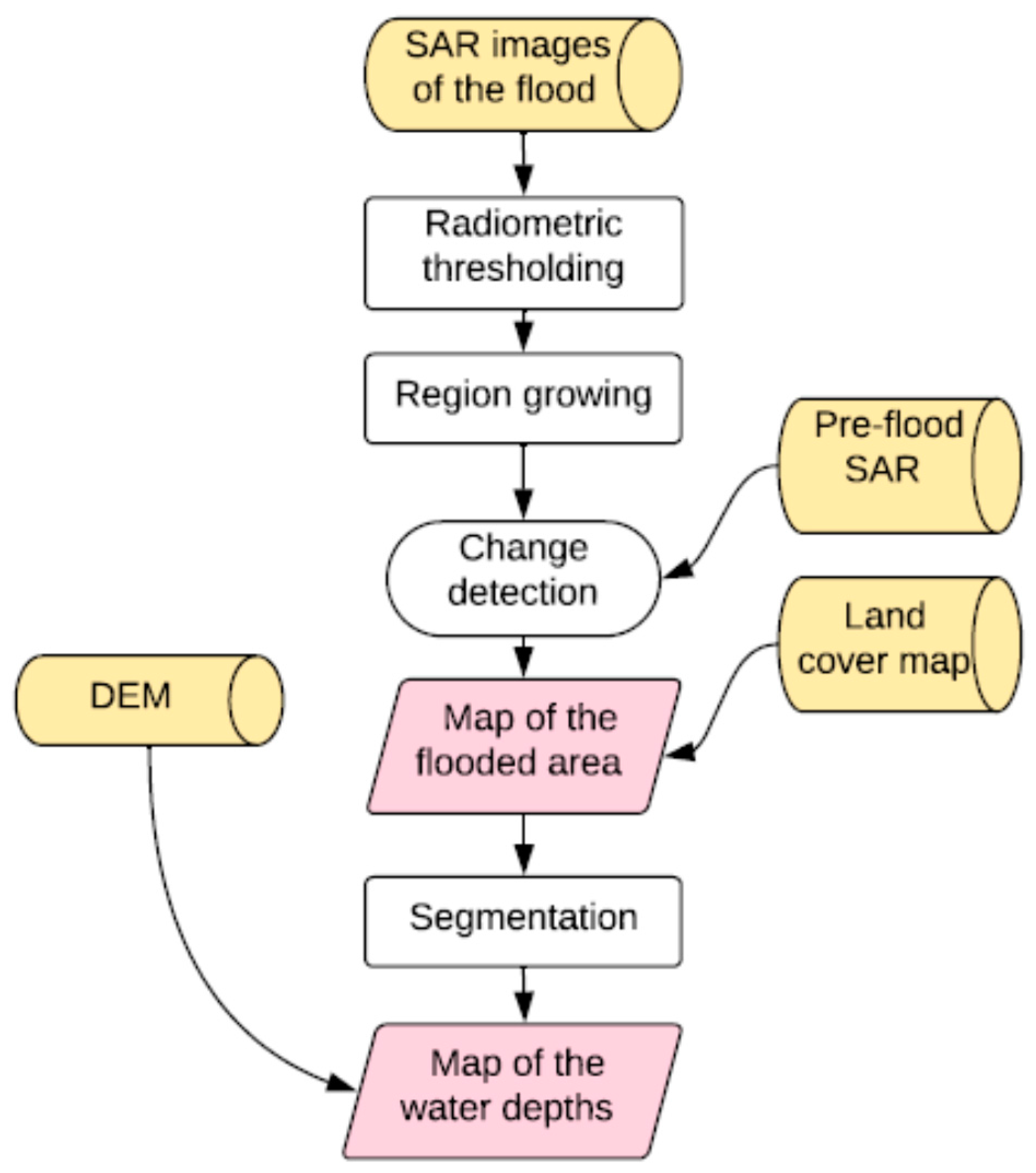
The proposed methodological framework, proposed in Figure 2, utilized to build the event scenarios for the Bradano case study and to monitor the spatio-temporal dynamic of floodplain drainage is described in this section. In particular, the section presents the flood mapping algorithms to extract flood extent layouts using SAR images (Section 3.1) that are, later, combined with a DEM in order to extract water-depth maps in a flat terrain with complex topography (Section 3.2). Subsequently, using these hazard-derived SAR and DEM images, acquired respectively near the flood peak and in the recession stage of the flood event, the processes adopted to constrain (at different floodplain points and in different time instants) a 2D hydraulic model (presented in Section 3.3), limiting the uncertainty of roughness parameters, are proposed in Section 3.4.

The methodology set out in this paper can be extended to reliable flood damage assessment for flood emergency management by increasing process automation levels. Operational products that are under development for accurate and timely flood risk assessment can address the growing need for knowledge transfer from science to practice through an open, transparent approach that is reliable, extensible, and participative ([30,31,32]).

3.1. SAR Image-Processing Algorithm for Flood Extent Extraction

The most commonly used SAR flood extent mapping techniques include simple visual interpretation (e.g., [33]), image texture algorithm [29], supervised classification and various multi-temporal change detection methods (e.g., [18,34]).

However, one of the most commonly adopted methods for distinguishing between flooded and non-flooded areas is the interpretation of radar signatures (e.g., [21,22]). The specular reflection of the radar signal is the main electromagnetic mechanism producing a high contrast in SAR images between flooded and non-flooded areas [14]. In general, floodwater that is covering the terrain is much smoother than the surrounding non-flooded land and reflects most of the impinging radar signal toward the specular direction, so backscatter is very low and flooded areas appear dark in shade [21]. This advantage of SAR data for flood mapping means computation efficiency for flood detection and monitoring algorithms that could make them suitable for supporting delineation of flood hazard scenarios requiring emergency management. Conversely, inundation mapping may be complicated by wind roughening and by vegetation emerging from water, producing high radar return that decreases the contrast between flooded and non-flooded areas in SAR images: for example, the scattering from a well-developed canopy becomes predominant and the presence of the underlying water is hardly detected by the radar [21].

In this light, the flood mapping procedure utilized in this study is basically a semi-automatic classification in which the integration of different rules is performed based not only on SAR but also on ancillary data, such as knowledge of land cover and information derived from a reference pre-flood SAR image.

The utilized methodology for flood extent extraction follows the steps proposed by [18]. It is comprises (i) SAR image radiometric thresholding to extract the water body core, (ii) a region-growing approach in which the backscatter of image pixels is compared to check the similarity with the value of the nearest neighbor seed pixel, i.e., bodies of water, in order to extract all areas covered by water; finally, the utilized approach takes advantage of (iii) SAR change detection capabilities by exploiting two images acquired before and during the flood to monitor backscattering changes caused by the flood event. Change detection thus aims to remove from the flood extent map pixels that do not correspond to floodwater. To do so, only pixels that change their backscatter values significantly with respect to their baseline values are kept in the final flood extent map [18].

By using a couple of SAR images (one flooded and one unflooded) change detection can reduce the false alarm probability arising from shadow areas, which appear as dark as the flooded pixels. Only pixels that change their backscatter values significantly in the two images are kept in the flood extent. RGB composition is used for this end: pre-flood and post-flood images are co-registered, each to a single master scene, and are combined into a color image to identify the flooded areas better in comparison to permanent water and other classes. SAR intensity images were filtered through a Lee filter [35], also with an 11 × 11 sliding window pixel size, and then converted to a logarithmic scale. Subsequently, a numerical comparison of the different values of the two SAR images distinguishes between flooded and unflooded areas more easily. This scheme was used extensively in past literature studies (see [18,23,34]), but it can be complicated by a wealth of other factors influencing the actual backscattering level of the terrain, which include surface roughness and soil moisture for land areas, the presence of capillary waves for bodies of water, or the presence of rain during acquisition. For example, wind may cause capillary waves in free water surfaces of large size, which may then increase the local backscatter level of SAR images. Moreover, the speckle noise inherent to all the coherent imaging devices causes statistical fluctuations in the backscattering levels of single pixels. All of these factors often become critical during flood events so the knowledge of land cover at 1:5000 scale, available from the Regione Basilicata geoportal (http://rsdi.regione.basilicata.it/) and detailed at finer scale through an orthophoto visual interpretation, was utilized by an operator to understand, for example, if it was necessary to look for dark spots in the image (bare soil) or to some increase in intensity with respect to an image taken before the flood event (e.g., over forested areas). Although the proposed procedure aims to make radar interpretation as automatic as possible, a certain degree of supervision by an expert operator was considered to be essential to reduce uncertainties arising in SAR flood mapping. For example, the presence of permanent tree vegetation, characterized by low penetration of electromagnetic waves through leaves and branches, makes it difficult to detect the presence of water below the canopy. Indeed, taking into account that (i) mapping flooded vegetation can be still considered a critical issue for operational inundation mapping using SAR data [36] and (ii) being aware that the aim of the proposed research is to contribute to scientific knowledge in the field of operational methods and models for real-time flood damage assessment, the area inside the river channel and the pinewoods that is closer to the river mouth were excluded from the calibration. Indeed, these parts of the study area are characterized by the presence of very dense and high vegetation without involving vulnerable elements so floods cannot produce direct damage in these zones.

3.2. Water Depth Estimation Combining SAR Images and a Digital Elevation Model

Although exploitation of river inundation satellite images, especially for operational applications, is mostly restricted to flood extent mapping, there is significant potential for improvement in a three-dimensional characterization of floods (i.e., flood-depth maps) using SAR satellite images.

When considering that estimation of water levels plays an essential role in quantifying potential flood event damage so control action can be taken during the emergency phase ([37]), the flood extent limits extracted by the SAR image here were combined with a Digital Elevation Model (DEM) allowing extraction of the terrain elevations inside all relevant limits and, thus, the estimation of elevation difference intervals across the surrounding topography (within the flood limits).

The Basilicata Basin Interregional Authority provided the authors with a plano-altimetric survey of the study area using laser-scanning technology and digital aerial photogrammetry. The airborne laser scanner system is an active remote-sensing sensor technique, that couples a laser attached to an aircraft with precise kinematic positioning provided by a differential global positioning system (DGPS) to produce accurate elevation measurements [38]. Data acquired from the Bradano River mouth area was formulated by a Topeye MKII system, which works in full waveform in order to provide a better description of all ground elements. Indeed, it is able to record multiple echoes besides the first and the last pulse ([39,40]). In area characterized by more complex topography, a flight was made at 600 m with an orthophotos resolution of 5 cm and a laser density of 40 pt/m². The resulting laser scanner points cloud had a vertical accuracy of about 0.15 m and horizontal accuracy of 0.30 m. When considering that the increase of DEM resolution corresponds to exponential computational time growth in hydraulic model simulation performance, it was considered appropriate to guarantee high altimetric detail of the hydraulic elements that have most influence on water flow (such as river reach dimension, cross-sections, banks, and levees, etc.), through manual manipulation rather than using an excessively detailed DEM grid resolution size [41]. Therefore, a square grid of 10 m resolution was used for input of the 2D hydraulic model, while the geometries of the most important hydraulic elements were entered in the grid to maintain good characterization of study area topography. Indeed, resolution should be chosen in relation to model structure and complexity, which always have limitations [42]. For instance, the FLORA-2D model cannot include inertial terms in governing equations, and therefore has low sensitivity to small-scale DEM features, meaning that close field flow processes are smoothed out, even when high-resolution grids are used [43].

Finally, it is important to note that finer grid resolution would require a more complex parameterization of the 2D hydrodynamic model, and, as consequence, it could increase the uncertainty of head losses and roughness [44]. Within this framework, the method for incorporating available topographic data into the model structure is the key to achieving the best compromise between detail (or precisions), maximum expected accuracy (which depends more on available dataset than on grid resolution), and computational efficiency [42]. In our opinion, the use of subgrid treatments, when combined with appropriate upscaling of resistance parameters, would, in many instances, be a suitable approach to making better use of available topographic details, while being consistent with the uncertainty related to model structure and other input data available for model-building and evaluation.

Previous studies (e.g., [10]) have derived water levels by computing the differences in elevation between each grid cell and the elevations of the flowpath-connected downslope grid cell where the flow enters the channel. This method is based on the law stating that hydraulic energy decreases from upstream to downstream. Using the assumption of one-dimensional (1D) modeling on flow direction, Hostache et al. [10] successfully determined a hydraulic hierarchy, composed of an up/downstream relationship between points of water-level estimation, corresponding to the sites of relevant limits. Consequently, following this approach, the water-level estimates in an area with gentle relief imply significant uncertainty. Thus, the method proposed in [10] cannot be applied with good results in extremely flat area where the extent of the flooded area is calculated through water transfer from neighboring cells alongside and perpendicular to the river.

In flat topography, the water level usually coincides with terrain elevation on the cells where there is wet–dry shift, i.e., on the relevant flood limits, with gradual floodwater depth increase moving away from these boundary cells. It is particularly true in areas with complex topography where water flow is confined by structural elements (e.g., levees, banks, bridges).

In this study, a three-step method is proposed for water-depth assessment in flat areas with complex topography. First, (i) the segmentation of the flood extent extracted from the SAR images is performed to localize the flooded area (segmentation block), which makes it possible to assume uniform flow, i.e., a horizontal water level. While the river channel is characterized by a slope oriented in the direction of the water flow, the complex topography (i.e., levees, embarkments etc.) of the floodplain area can confine water flow, which may be stagnant in some points as identified by the SAR images in different moments of the flood event. Since the segmentation step is not the primary aim of this paper, an expert operator used orthophoto maps to identify the presence of overhead structural elements (typically non-flooded cells) able to confine water flow. Next, (ii) the maximum water level of each segmentation block was estimated as the mean of the terrain elevation values included in a 95–100 percentile range of the DEM cells that are located along the boundaries of the analyzed block; Finally, (iii) the water depth of each pixel within the considered block was evaluated as the difference between the water level value estimated in the previous step and the terrain elevation values of the cells.

3.3. Flood Inundation Modeling

In this study, the FLORA-2D hydraulic model [45] was used to simulate flood dynamics and the extent of two Bradano River flood scenarios referred, respectively, to November 2010 and December 2013, described in Section 2. The two-dimensional hydrodynamic model, already proposed in [45], is based on the numerical solution of a simplified subset of an equation derived from Navier-Stokes shallow water equation formulation. It was developed with the aim of simulating flood propagation in flat areas, taking into consideration the dynamic spatio-temporal effect of vegetation. Indeed, the topography and land-use roughness are the most critical factors in 2D hydraulic modeling [46], as they influence estimation of flood extension and its flow characteristics, like water depth that can be considered the main factor of flood losses according to [9]. The numerical solution was developed for the specific needs of providing a good compromise between simulation time and data accuracy for a correct representation of the process [37], namely to obtain high computational efficiency through the use of a simplified set of initial and boundary conditions.

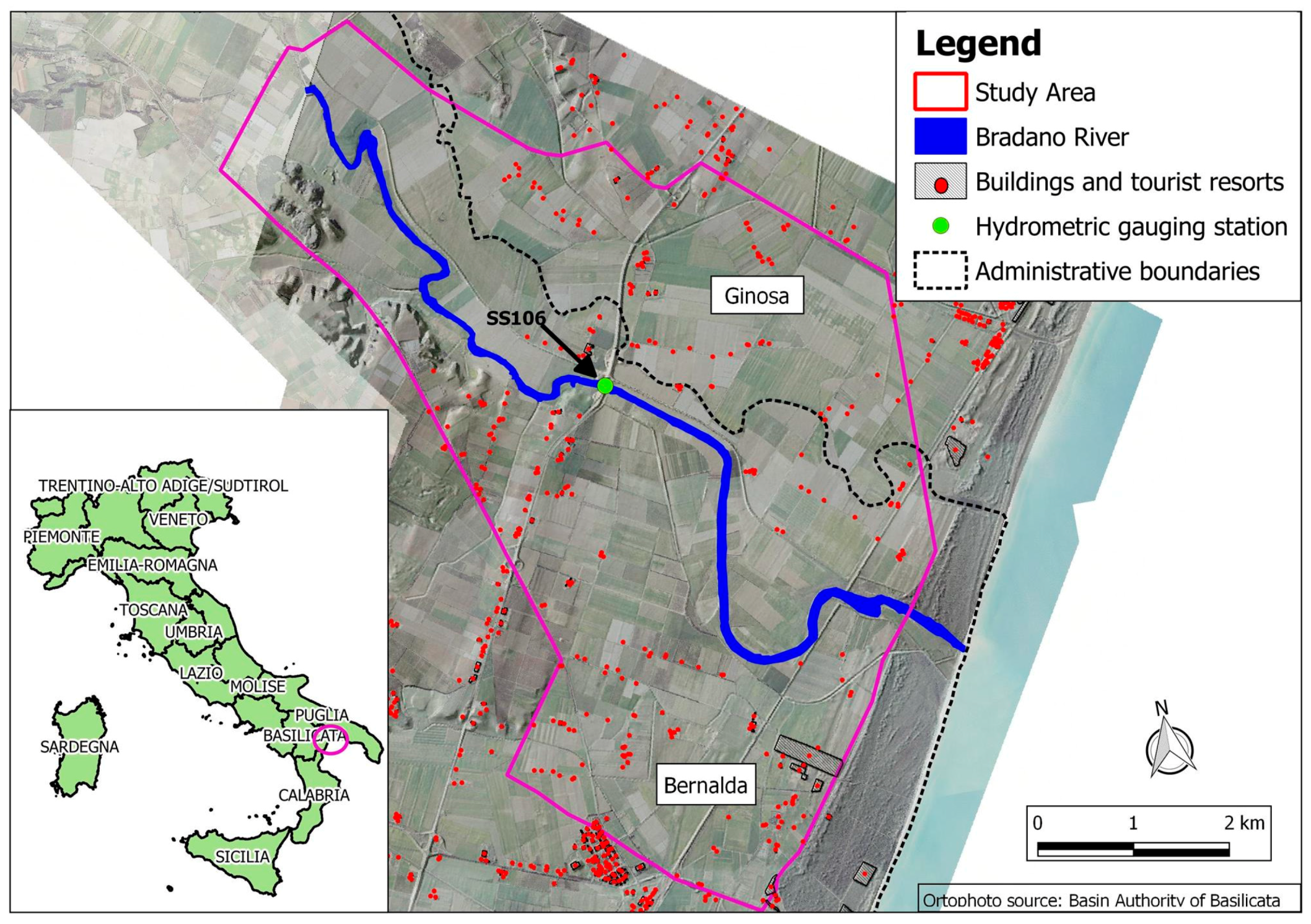
The initial flood stage condition was a null riverbed water level. Moreover, the upstream boundary condition was constructed by considering the effective water depth measurements along the river, available as readings from a gauge station in the analysis area, called S.S. 106 (see Figure 1). Conversely, in [45,47] the authors used the output of the hydrological model as a boundary condition simulating FLORA-2D for the 1 March 2013 Bradano flood event, (not analyzed in this study), because the information that was recorded by the S.S.106 hydrometric station was not available due to malfunctions caused by the impact of the flood. The above-mentioned hydrometric levels were assigned as upstream boundary conditions, while a constant water level equal to 0.5 m a.s.l. was considered a downstream boundary condition (sea level was assumed to be slightly above standard conditions). Finally, the spatial distribution of flow resistance was derived from LiDAR data, used to generate maps of vegetation heights [48]. In this application, the computational domain was defined by a square grid with a resolution of 10 m, while the time step was set to 2 s to ensure model stability.

3.4. Hydraulic Model Calibration Framework Using SAR- and DEM-Derived Flood Maps

Several studies have pointed to hydraulic roughness as a dominant factor for relatively shallow inundation ([10,49,50,51]) in particular for 2D hydraulic models ([25,52]), as it can affect flood extent, timing of flood waves, and localized processes such as location of hydraulic leaps. Moreover, recent research has highlighted that roughness parameters are the chief factors in deciding the rate of flooding and receding, and thus their calibration heavily depends on the timing of the SAR images ([15,53]) during model calibration as in the proposed study. Hence, we decided to restrict FLORA-2D model calibration to Manning coefficients considered the most important parameters, but also the main source of uncertainty ([43,54]), especially in an area with a gentle and flat topography where we can consider that friction and ground slope in a gravity wave have the same order of magnitude within the energy equation, controlling flow characteristics even though it is acknowledged that several parameters (e.g., related to roughness, channel cross-section dimensions, initial condition) can influence model results.

In particular, the Manning (roughness) coefficient is a spatio-temporally-distributed parameter that changes over space (e.g., bed channel versus vegetated floodplains) and time (e.g., seasonal changes of vegetation or temporal resistance variation due to vegetation). However, variable spatio-temporal Manning coefficients of this kind cannot be measured in real world applications [15]. Moreover, this parameter is generally determined under uniform flow conditions rarely observed in an area characterized by flat and complex topography.

Thus, Manning coefficient values are regarded in literature as parameters that may vary widely. Classes of coefficient have been drawn up for the different land use categories to be used as parameters, which are estimated using model calibration.

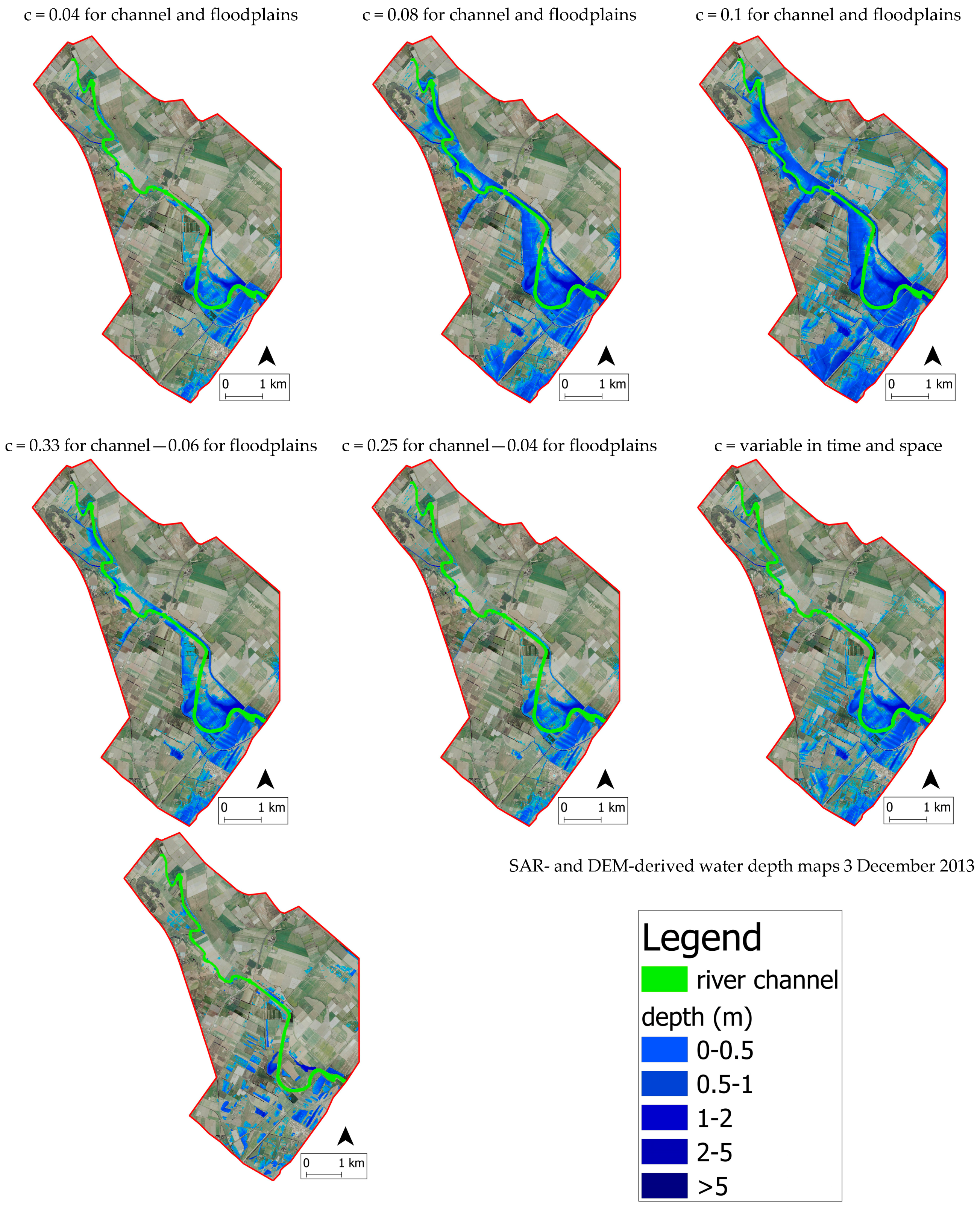
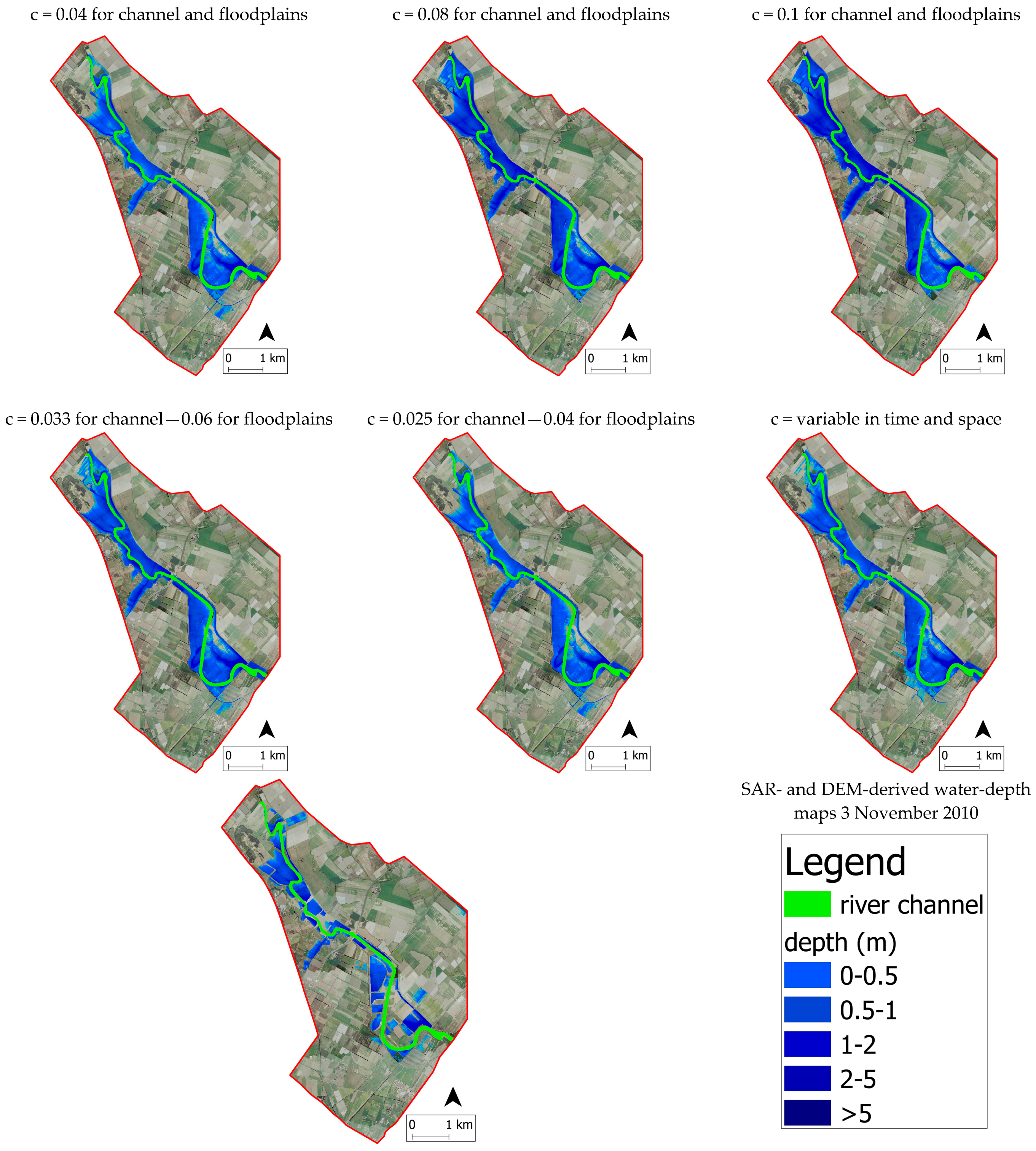
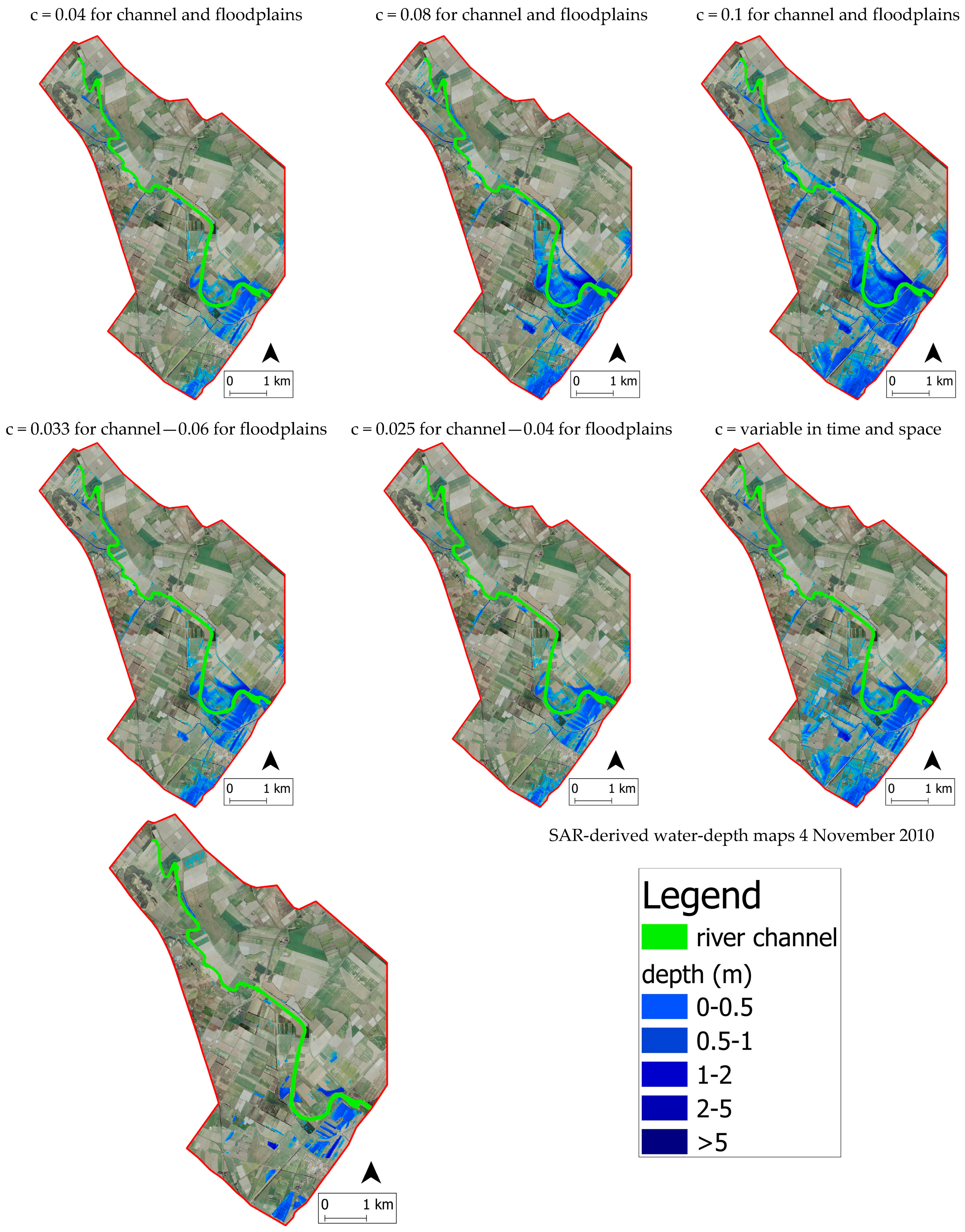
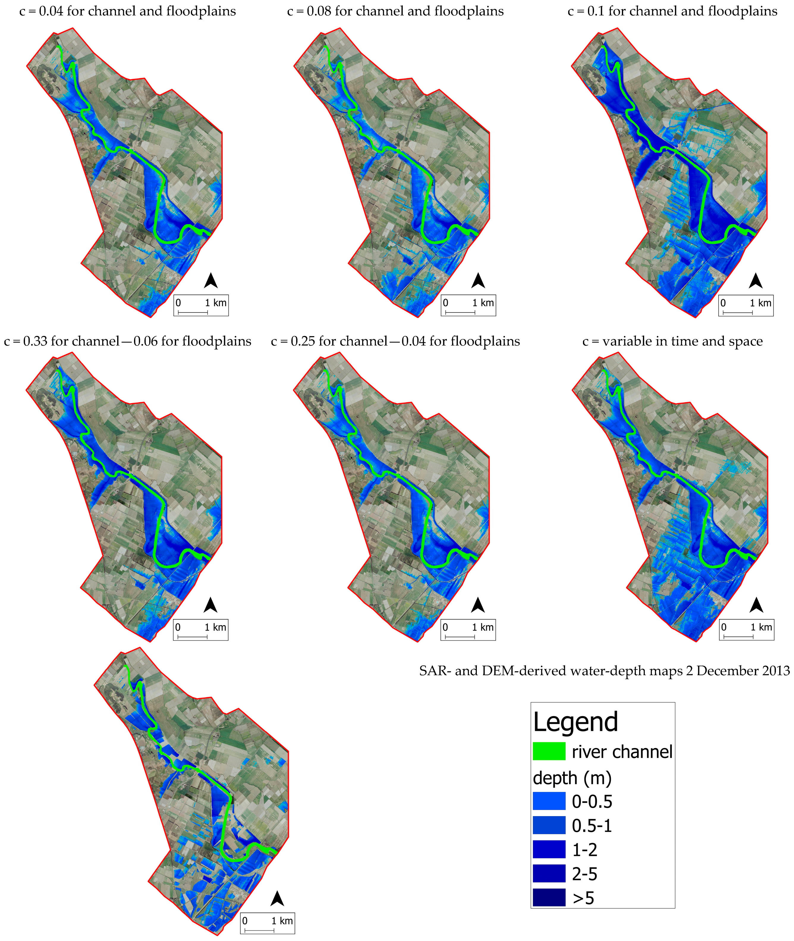
For this purpose, a set of model runs corresponding to a set of plausible Manning coefficient values was carried out, assuming that the Manning roughness values may lie between 0.04 and 0.1. A low roughness coefficient of 0.04 represents quite a clean channel, i.e., covered by grassland, whereas a high roughness coefficient of 0.1 would represent a channel with very thick vegetation. We therefore performed three simulations with roughness coefficients, respectively, of 0.04, 0.08, and 0.1 for the whole area. Later, we distinguished between the Manning coefficients in the main channel and floodplain assuming they were temporally and spatially constant. When considering that the Manning coefficient for the channel was higher than in the floodplain, we performed another two simulations that has, respectively, (i) a Manning coefficient value of 0.033 in the channel and 0.06 elsewhere, representing a wet season; and, (ii) 0.025 in the main channel and 0.04 in the floodplains, representing a dry season in which vegetation is quite sparse and low.

In this way, Manning coefficient values in the floodplain, which can be considered the area of greatest influence due to its sheer extension, varied in regular steps of 0.02 in these five simulations (i.e., 0.04, 0.06, 0.08, 0.1). Finally, for the last hydraulic simulation, we used variable spatio-temporal Manning coefficients that can take into consideration the dynamic effects of vegetation: cell roughness varies with floodwater depth according to a low that depends on the type of vegetation, as in [45]. In particular, Manning coefficient n is calculated according to [55] when vegetation is rigid, and [56] in the case of flexible vegetation. The step size for the Manning coefficient was explored over a fixed grid of 10 m cell resolution for all of the model runs.

To emphasize the integration of SAR-derived datasets instead of traditional calibration data, e.g., hydrographs, a two-step approach was adopted.

The first step of the calibration procedure is based on flood extent maps derived from a temporal series of SAR images (resampled, avoiding unsustainable computational times, at the same resolution as the hydraulic model, i.e., 10 m) for the 3–4 November 2010 Bradano event. The FLORA-2D hydraulic model does not have a routine that is able to simulate soil water infiltration and does not therefore account for soil permeability. Hence, water-depth values of less than 0.1 m could be not considered to be significant in the model results because cannot influence assessment of flood losses [9]. To guarantee the consistency of calibration and validation processes, the pixels in the SAR- and DEM-derived and in the hydraulic model flood maps were labeled as flooded where water depth exceeded 0.1 m.

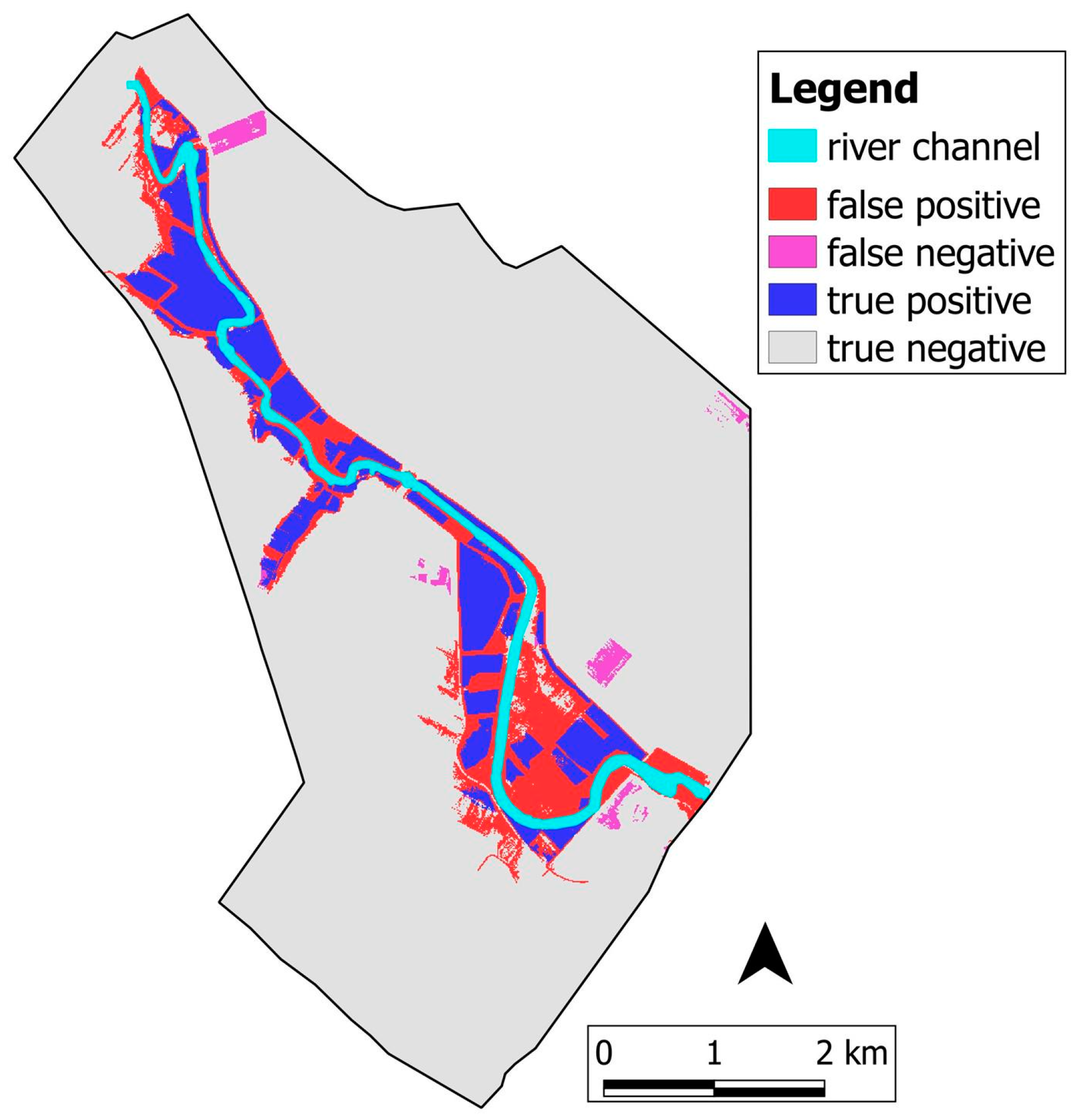
When comparing each SAR-derived map pixel to pixel with the flood map obtained with the hydraulic model at the same time step, there were four possible conditions in each map point/cell: (i) if the hydraulic model detected a flooded area when this condition was present in the SAR-derived flood map, the point was counted as a true positive; otherwise; (ii) if it identified a point as non-flooded (negative), it was counted as a false negative; (iii) if the site was defined non-flooded by the SAR map and classified as negative, it was counted as a true negative; otherwise, (iv) if it was classified as positive, it was counted as a false positive. From this, the true positive rate (also called hit rate) was estimated as:

$$r_{fp}\approx \frac{Positivecorrectlyclassified}{Totalpositives}$$

(1)

The false positive rate (also called false alarm rate) was:

$$r_{fp}\approx \frac{Negativesincorrectlyclassified}{Totalnegatives}$$

(2)

The proposed contingent matrix is similar to a confusion matrix and is successfully and widely used in the field of flood susceptibility assessment, e.g., in [18,47,57,58,59].

Moreover, the performance measurement, used to give a deterministic indication on how well each FLORA-2D-simulated flood map represented the SAR-derived flood extent map was obtained by minimizing the sum $r_{fp}+\left(1-r_{tp}\right)$ in the different time instants that were considered, of the false positive rate, i.e., error type 1, and the false negative rate, i.e., error type 2, assigning equal weights to the two rates. The sum of the two errors represents an objective function that can be used for calibration purposes ([47,58]), hereafter called minimized sum of errors (MSE).

The outcomes of the performance measurement evaluated through the comparison between a SAR-derived flood map and the flood map obtained by the hydraulic model at the same time step, were used in the following equation to identify the hydraulic model run concordance and discordance with respect to SAR-derived flood maps:

$$\raisebox{1ex}{${{\displaystyle \sum }}_i^n\left(MS{E}_{t_i}^{c_j}\right)$}\!\left/ \!\raisebox{-1ex}{${{\displaystyle \sum }}_i^n\left(MSEmi{n}_{t_i}\right)$}\right.$$

(3)

where $MS{E}_{t_i}^{c_j}$ is the MSE value obtained by pixel-to-pixel comparison of each FLORA-2D-simulated flood extent map computed with a roughness coefficient of c_j and the SAR-derived map for a CSK revisit time of t_i; $MSEmi{n}_{t_i}$ is the minimum value of all the MSE values, at the same t_i temporal instant, associated to all FLORA-2D-simulation runs characterized by different values of the c_j Manning coefficient. The equation outcome (Equation (3)) was used to judge the performance of the hydraulic model runs.

In the second step, the remotely sensed water levels were integrated to enhance the hydraulic model calibration. We compared the water depth maps of the concordance model run sets selected in the first step with floodwater depth extracted, as described in Section 3.2, by combining SAR images and the Digital Elevation Model. Floodwater depth maps were compared pixel to pixel to see if there was concordance or discordance between the two paired maps, i.e., the SAR- and DEM-derived map and the water depth map simulated by the hydraulic model, using root square mean errors (RSME) and the Nash and Sutcliffe efficiency coefficient (NSE), whose formulation is shown below for measuring proper fit [60].

$$RMSE=\sqrt{N^{-1}{{\displaystyle \sum }}_i^N{\left(P_i-O_i\right)}^2}$$

(4)

$$NSE=1-\frac{{{\displaystyle \sum }}_i^N{\left(O_i-P_i\right)}^2}{{{\displaystyle \sum }}_i^N{\left(O_i-\overline{O}\right)}^2}$$

(5)

where $P_i$ and $O_i$ represent the predicted (simulated by the hydraulic model) and observed SAR values, respectively, and $\overline{O}$ is the mean of the observed value. The resulting best performance of Manning roughness parameters that were obtained during this calibration process were then used for model validation purposes for the 2–3 December 2013 Bradano flood event scenario to evaluate calibrated model robustness under different operating conditions.

4. Results and Discussion

4.1. Model Calibration

Model calibration is essential for checking model performance before it can reasonably be used for near real-time flood forecasting and monitoring or for flood risk management in general [60].

The FLORA-2D hydrodynamic model was calibrated using the 3–4 November 2010 Bradano River flood event, with flood hazard maps derived from the two SAR images acquired, respectively, at 4:47 a.m. of 3 November 2010 (during the rising phase of the event) and at 4:47 a.m. of 4 November 2010 (during the recession phase of the flood event). As stated before (Section 3.4), model calibration was performed over six different sets of channel and floodplain Manning coefficients, since the roughness parameters determine mainly flooding and receding rate in a flat area with complex topography [15].

Firstly, the performance of each model simulation was analyzed in terms of flood extent, when comparing these simulated flood hazard maps (pixel to pixel) with the temporal series of SAR images at the same time step. As shown in Figure 3, the result of the comparison of each flood extent map simulated with a FLORA-2D model, characterized by a specific set of Manning coefficients, and the SAR-derived flood extent map at the same time step, produced a matrix (or contingency table) of four possible outcomes. Taking the SAR-derived maps as a reference, there are two ways for the hydraulic simulated flooded area to be correct (either by representing flooded or non-flooded pixels correctly) and two ways to be incorrect (either by erroneously under- or over-predicting the observed inundation extent).

To provide a quantitative description of the efficacy of each hydraulic simulation, we summarize in

Table 2. Results of the calibration performance of the hydraulic simulation model for 3 November 2010 in terms of a flood extent map: the set of Manning coefficients c, false positive rate $r_{fp}$, true positive rate $r_{tp}$, false negative rate $r_{fn}$, minimized sum of errors (MSE), and accuracy, sensitivity, and specificity.

Statistical Performance Measurements of Flood-Extent Estimation 3 November 2010
	${\mathit{r}}_{\mathit{f}\mathit{p}}$	${\mathit{r}}_{\mathit{t}\mathit{p}}$	${\mathit{r}}_{\mathit{f}\mathit{n}}$	MSE	Accuracy	Sensitivity	Specificity
c
0.04 for channel and floodplains	7.71	85.02	14.98	22.69	91.64	85.02	92.29
0.08 for channel and floodplains	9.69	86.01	13.99	23.68	89.93	86.01	90.31
0.1 for channel and floodplains	9.62	83.92	16.08	25.7	89.8	83.92	90.38
0.33 for channel and 0.06 for floodplains	9.39	85.97	14.03	23.42	90.19	85.97	90.61
0.025 for channel and 0.01 for floodplains	7.59	84.76	15.24	22.83	91.72	84.76	92.41
variable in time and space	9.24	86.91	13.09	22.33	90.41	86.91	90.76

and

Table 3. Results of the hydraulic simulation model calibration performance for 4 November 2010 in terms of the flood extent map: the set of Manning coefficients c, false positive rate $r_{fp}$, true positive rate $r_{tp}$, false negative rate $r_{fn}$, minimized sum of errors (MSE), and accuracy, sensitivity, and specificity.

Statistical Performance Measurement of Flood-Extent Estimation 4 November 2010
	${\mathit{r}}_{\mathit{f}\mathit{p}}$	${\mathit{r}}_{\mathit{t}\mathit{p}}$	${\mathit{r}}_{\mathit{f}\mathit{n}}$	MSE	Accuracy	Sensitivity	Specificity
c
0.04 for channels and floodplains	7.08	72.11	27.89	34.97	92.13	72.11	92.92
0.08 for channel and floodplains	14.04	81.76	18.24	32.28	85.8	81.76	85.96
0.1 for channel and floodplains	21.28	86.18	13.82	35.1	79.011	86.18	78.72
0.33 for channel and 0.06 for floodplains	9.96	78.45	24.55	34.51	89.6	78.45	90.04
0.025 for channel and 0.01 for floodplains	6.96	71.63	28.37	35.33	92.22	71.63	93.04
variable in time and space	16.88	87.6	12.4	29.28	83.29	87.6	83.12

the performance of each defined set of Manning coefficients investigated, respectively, by a comparison with the two SAR images acquired during 3 November and 4 November 2010. The optimal performance values for each time step were identified by utilizing the above-mentioned minimized sum of errors (MSE). In particular, Table 2 and Table 3 provide the following information: the relative value of the Manning coefficients c, the false positive rate $r_{fp}$, the true positive rate $r_{tp}$, false negative rate $r_{fn}$, the minimized sum of errors (MSE), and some additional statistical performance measurements, such as accuracy, sensitivity, and specificity for each hydraulic simulation. Sensitivity (also referred to as “recall”) refers to the proportion of correctly classified instants of flood pixels, whereas Specificity evaluates the proportion of correctly classified instants of non-flood pixels. Accuracy refers to the proportion of pixels that are classified correctly. Sensitivity, Specificity, and Accuracy are calculated using the following formulas [57]:

$$Sensitivity=\frac{TP}{TP+FN}$$

(6)

$$Specificity=\frac{TN}{FP+TN}$$

(7)

$$Accuracy=\frac{TP+TN}{TP+TN+FB+FN}$$

(8)

where TP is true positive and defined as the total number of pixels predicted positive that are positive; FR is false positive and equal to the number of pixels predicted positive that are negative; TN is true negative and equal to the number of pixels predicted negative that are negative; and, finally, FN is false negative and equal to the number of pixels predicted negative that are positive.

Ground truth information was not available for calibration purposes, but Table 2 and Table 3 show concordance between SAR-derived and hydraulic model-derived maps, in terms of false positive rate, i.e., error type 1, which varies in the range 7–20% and the false negative rate, i.e., error type 2, that varies in the range 12–28%, and can be considered an indication of the reliability of products generated to perform the flood extent assessment.

The value of the sum of each minimized sum of errors (MSE) for the various time steps (i.e., 3 and 4 November 2010) was lowest for the hydraulic simulation using variable Manning time-and-space coefficients c as compared to all of the other simulations. It was seen that variable Manning time-and-space coefficients c estimated observed data better than all the others, while all of the simulations put in place showed good performance in terms of flood extent maps during the 3–4 November 2010 flood event. Moreover, the results obtained highlighted the highest information content that could be found in those SAR flood maps that were acquired near the peak of the flood hydrograph and improved when more images were combined.

In the second calibration step, SAR- and DEM-derived water levels were integrated to enhance the hydraulic model calibration. The remotely sensed images were converted into floodwater depth maps, as described in Section 3.2. Taking the SAR-derived maps as reference and considering only the overlap between the SAR-derived and model flooded area, the overall accuracy, the root square mean errors (RSME) and the Nash and Sutcliffe efficiency (NSE) coefficients were used to compute for both the 3 and 4 November 2010 timeframes. As seen in

Table 4. Results of the calibration performance of the hydraulic simulation model for 3 November 2010 in terms of water depth: the relative value of Manning coefficients c, Root Mean Square Error RMSE, Nash- Sutcliffe Efficiency Coefficient (NSE), coefficient of determination R², Unsystematic RSME RSMEu, fraction bias FB, prediction within a factor of two of observation FA2.

Statistical Performance Measurements of Water-Depth Estimation 3 November 2010
	RSME (m)	NSE	R2	RSMEu (m)	FB	FA2
c
0.04 for channel and floodplains	0.39	0.53	0.64	0.46	0.21	0.84
0.08 for channel and floodplains	0.50	0.22	0.51	0.45	−0.26	0.78
0.1 for channel and floodplains	0.68	−0.41	0.24	0.47	−0.34	0.66
0.033 for channel and 0.06 for floodplains	0.36	0.61	0.63	0.45	−0.76	0.88
0.025 for channel and 0.01 for floodplains	0.40	0.50	0.64	0.45	0.23	0.82
variable in time and space	0.32	0.69	0.7	0.45	0.06	0.91

and

Table 5. Results of the calibration performance of the hydraulic simulation model for 3 November 2010: the relative value of Manning coefficients c, Root Mean Square Error RMSE, Nash- Sutcliffe Efficiency Coefficient (NSE), coefficient of determination R², Unsystematic RSME RSMEu, fraction bias FB, prediction within a factor of two of observation FA2.

Statistical Performance Measurements of Water-Depths Estimation 4 November 2010
	RSME (m)	NSE	R2	RSMEu (m)	FB	FA2
c
0.04 for channel and floodplains	0.30	0.28	0.70	0.25	0.37	0.81
0.08 for channel and floodplains	0.27	0.50	0.68	0.44	−0.16	0.93
0.1 for channel and floodplains	0.37	0.07	0.64	0.46	−0.32	0.84
0.033 for channel and 0.06 for floodplains	0.26	0.53	0.57	0.34	0.08	0.91
0.025 for channel and 0.01 for floodplains	0.31	0.22	0.69	0.24	0.4	0.8
variable in time and space	0.19	0.76	0.76	0.33	0.01	0.95

, the performance values of the hydraulic model vary widely depending on the basis of the set of the different Manning coefficient values utilized. It was seen that a successful depth calibration could only be obtained when channel roughness values were confined to a plausible range. Indeed, the performance of the simulation characterized by a Manning value of 0.1 in terms of both extent and water-depth maps, was the lowest, confirming literature theories that this value remains unexpectedly high [15]. It is also confirmed that is not realistic to find that Manning coefficient values for the channel are higher than those for the floodplain [26].

The comparable values (greater than 0.7) of the estimated coefficient of determination (R²) for the simulation with variable Manning time-and-space coefficients in all of the considered time steps indicated that this simulated scenario was in substantial agreement with the SAR observations performed on the subsequent days and that water recession as observed by SAR was consistent from the physical point of view. The coefficient of determination (R²) was calculated using the following formulas:

$$R^2={\left[\frac{{{\displaystyle \sum }}_{i=1}^n\left(O_i-\overline{O}\right)\left(P_i-\overline{P}\right)}{\sqrt{{{\displaystyle \sum }}_{i=1}^n{\left(O_i-\overline{O}\right)}^2}\sqrt{{{\displaystyle \sum }}_{i=1}^n{\left(P_i-\overline{P}\right)}^2}}\right]}^2$$

(9)

where 0_i and P_i are the observed SAR and DEM derived water levels and predicted by the hydraulic model of the ith cell, respectively; $\overline{O}$ and $\overline{P}$ are the means of the observed and simulated value. R² ranges from 0 to 1, where higher values represent good model performance, and R² > 0.5 is generally considered satisfactory [60].

Table 4 and Table 5 provide the following information: the relative value of the Manning coefficients c, Root Mean Square Error RMSE, Nash Efficiency Coefficient (NSE), coefficient of determination R², Unsystematic RSME RSMEu, fraction bias FB, prediction within a factor of two of observation FA2, i.e., fraction of data contained in the interval $0.5O_i<P_i<2.0O_i$. Unsystematic RSME and fraction bias are calculated using the following formulas:

$$RSM{E}_u=\sqrt{N^{-1}{{\displaystyle \sum }}_i^n{\left(P_i-\overline{P}\right)}^2}$$

(10)

$$FB=2\left(\overline{O}-\overline{P}\right)/\left(\overline{O}+\overline{P}\right)$$

(11)

In Figure 4 and Figure 5, water depth shows large variations, but also a clear spatial pattern. The areas where floodwater was still present during the SAR time series basically correspond to the more sunken areas, those where the largest water elevations were predicted by the hydrodynamic model.

Moreover, Figure 4 and Figure 5 reveal that when calibration is performed with an image that was obtained near the peak flow (3 November), the uncertainty of modeled extents increases with respect to the advanced recession phase (4 November) where water levels were less liable to change but the flood extent showed an increasing variation for the different Manning coefficient values. The low roughness coefficient values tend to fit well with the observed flood map in the first part of the event, while the water tends to recede faster respect to SAR-derived hazard maps during the recession phase. This is to be expected since changes in roughness would have an immediate and local impact on flood dynamics. The model responds to changes in channel friction by altering the speed of the flood wave and flow velocities consequently impacting the timing of flood wave propagation. If channel roughness were set too high, the flood wave would be delayed and if set too low, the flood wave would be too advanced, which explains the better performance of the variable spatio-temporal Manning coefficients with respect to others also in terms of water-depth evaluation.

4.2. Validation Performance Measures

Model validation is an extension of model calibration and is necessary for evaluating a model’s robustness under different operating conditions [60]. In this light, the selected sets of Manning coefficient values were used in the hydraulic model to formulate predictions for the 2–3 December 2013 Bradano River flood event. We could have excluded simulation runs showing poor performance during calibration, e.g., Manning coefficient value equal to 0.1, but we chose to show all of the results to demonstrate the robustness of the proposed approach. Hence, in

Table 6. Results of hydraulic simulation model calibration performance for 2 December 2013 in terms of a flood extent map: the set of Manning coefficients c, false positive rate $r_{fp}$, true positive rate $r_{tp}$, negative rate $r_{fn}$, minimized sum of errors (MSE), and accuracy, sensitivity, and specificity.

Statistical Performance Measurements of Flood-Extent Estimation 2 December 2013
	${\mathit{r}}_{\mathit{f}\mathit{p}}$	${\mathit{r}}_{\mathit{t}\mathit{p}}$	${\mathit{r}}_{\mathit{f}\mathit{n}}$	MSE	Accuracy	Sensitivity	Specificity
c
0.04 for channel and floodplains	10.35	66.07	33.93	44.28	85.17	66.07	89.65
0.08 for channel and floodplains	12.71	76.17	23.83	36.54	85.17	76.17	87.29
0.1 for channel and floodplains	30.52	92.55	7.45	37.97	73.86	92.55	64.48
0.033 for channel and 0.06 for floodplains	13.57	72.95	27.05	40.62	83.87	72.95	86.43
0.025 for channel and 0.01 for floodplains	10.17	65.88	34.12	44.29	85.28	65.88	89.89
variable in time and space	24.17	98.53	1.47	25.64	80.15	98.53	75.83

and

Table 7. Results of hydraulic simulation model calibration performance for 3 December 2013 in terms of a flood extent map: the set of Manning coefficients c, false positive rate $r_{fp}$, true positive rate $r_{tp}$, false negative rate $r_{fn}$, minimized sum of errors (MSE), and accuracy, sensitivity, and specificity.

Statistical Performance Measurements of Flood-Extent Estimation 3 December 2013
	${\mathit{r}}_{\mathit{f}\mathit{p}}$	${\mathit{r}}_{\mathit{t}\mathit{p}}$	${\mathit{r}}_{\mathit{f}\mathit{n}}$	MSE	Accuracy	Sensitivity	Specificity
c
0.04 for channel and floodplains	9.24	45.12	54.88	64.12	87.01	45.12	90.76
0.08 for channel and floodplains	20.7	70.37	29.63	50.33	78.57	70.37	79.3
0.1 for channel and floodplains	32.13	91.93	8.07	40.2	69.85	91.93	67.87
0.033 for channel and 0.06 for floodplains	14.05	52.74	47.26	61.31	83.22	52.74	85.95
0.025 for channel and 0.01 for floodplains	8.97	44.69	55.31	64.28	87.22	44.69	91.03
variable in time and space	18.16	81.27	18.73	36.89	81.79	81.27	81.84

, model performance in terms of flood extent detection are shown respectively for 2 December and 3 December 2013 timeframes, as we have done previously during calibration process. In general, Table 6 and Table 7 show an increasing variation and a decrease in performance in comparison with calibration performance results (see Table 2 and Table 3). As described in Section 2, the December 2013 event was of a great magnitude, in terms of precipitation intensity, and produced more damage with respect its predecessor in November 2010. Therefore, the uncertainty and sensitivity of the model increased with the increased magnitude of the event, as shown in Figure 6 and Figure 7. Moreover, in this case, the first SAR images (2 December) were acquired shortly after the peak flow and the second was in the advanced recession stage (3 December). During the initial recession, the routing of water was supported mainly by both spatial distribution of floodplain Manning coefficients and by downstream conditions and was less affected by the roughness of the river channel, generally less variable in time and space. Therefore, the preferred pre-peak observations are less sensitive to spatial roughness variation so the model performance is more uniform, as seen in Table 2 and Table 3.

It highlights that a tight sequence of images could improve model predictions. Combining observations in this way appears to focus the location of the roughness parameter more clearly than is possible using single images. Indeed, as listed in

Table 8. Results of hydraulic simulation model calibration performance for 2 December 2013 in terms of water depth: the relative value of the Manning coefficients c, Root Mean Square Error RMSE, Nash- Sutcliffe Efficiency Coefficient (NSE), coefficient of determination R², Unsystematic RSME RSMEu, fraction bias FB, prediction within a factor of two of observation FA2.

Statistical Performance Measurements of Water-Depths Estimation 2 December 2013
	RSME (m)	NSE	R2	RSMEu (m)	FB	FA2
c
0.04 for channel and floodplains	0.40	0.19	0.51	0.44	0.26	0.79
0.08 for channel and floodplains	0.46	−0.16	0.52	0.42	0.43	0.63
0.1 for channel and floodplains	0.61	−0.89	0.58	0.68	−0.41	0.77
0.033 for channel and 0.06 for floodplains	0.34	0.42	0.57	0.50	−0.05	0.84
0.025 for channel and 0.01 for floodplains	0.40	0.15	0.52	0.43	0.28	0.78
variable in time and space	0.26	0.65	0.71	0.45	−0.09	0.93

and

Table 9. Results of hydraulic simulation model calibration performance for 3 December 2013: the relative value of the Manning coefficients c, Root Mean Square Error RMSE, Nash- Sutcliffe Efficiency Coefficient (NSE), coefficient of determination R², Unsystematic RSME RSMEu, fraction bias FB, prediction within a factor of two of observation FA2.

Statistical Performance Measurements of Water Depths Estimation 3 December 2013
	RSME (m)	NSE	R2	RSMEu (m)	FB	FA2
c
0.04 for channel and floodplains	0.32	0.55	0.6	0.38	0.16	0.79
0.08 for channel and floodplains	0.33	0.42	0.7	0.48	−0.30	0.74
0.1 for channel and floodplains	0.43	−0.15	0.6	0.51	−0.42	0.58
0.033 for channel and 0.06 for floodplains	0.21	0.70	0.74	0.43	−0.10	0.81
0.025 for channel and 0.01 for floodplains	0.33	0.51	0.51	0.36	0.18	0.77
variable in time and space	0.22	0.72	0.8	0.41	0.04	0.83

, values greater than 0.65 of the estimated NSE efficiency coefficient and the low value of the RMSE (varying between 0.04 and 0.07) for simulation with variable spatio-temporal Manning coefficients shows, in all of the considered time steps, that this model-predicted scenario was in substantial agreement with the SAR observations performed on subsequent days in the validation period.

In both timeframes (i.e., 2 and 3 December) most of the simulation model errors with variable roughness were unsystematic, as shown by the comparison of RSME and RSMEu. The tendency to overestimate was confirmed by a positive FB value, although the response was spatially variable and areas of under-prediction also occurred. Over-prediction areas tend to affect related floodplain areas that drain rapidly along particular drainage stretches or where backwater effects cannot be derived by combining SAR and DEM in flat areas with complex topography. Over-prediction is not surprising since the hydrodynamic model’s failure to include hydrological components of the floodplain mass balance (infiltration, direct precipitation, evapotranspiration, and local runoff) and considering the tendency to be bordered by relatively dense vegetation which increases height errors, e.g., in zones closer to the channel meander in the river mouth. These features clearly merit further investigation, however it is more likely that the deterioration in model performance during floodplain dewatering was due to failure to characterize minor floodplain drainage channels correctly within the model or to inherent deficiencies in model formulation, as highlighted in [61]. Moreover, the high FA2 values confirm the successful adaptation of the model to observed SAR-derived data. However, the better performance of calibration results with respect to validation outcomes in term of statistical measurements could be due to the lower magnitude of the event that was analyzed during the calibration, and, as consequence, the lower spatial extension of the flood event that may simply be easier to predict by hydrodynamic model; the difference between calibration and validation statistical performances could also due to the fact that the uncertainties in the model results could be proportional to the amount of the analyzed flooded cells.

Observing calibration and validation results, it can be concluded that the FLORA-2D model, using variable spatio-temporal Manning coefficient values, successfully simulated the dynamics of the flood events considered, in terms of flood extent and water depth maps. In particular, the value of the Nash-Sutcliffe Efficiency coefficient, as obtained by comparing the results of variable spatio-temporal Manning coefficient simulation and SAR- and DEM-derived water depth maps, is on average equal to 0.7, which can be considered to be satisfactory for distributed models according to [60].

The channel roughness parameter c was less sensitive to variations in flood extent than water depth in both the calibration and validation period. By constraining c values to a more plausible range through calibration, it was possible to improve validation performance and further improve the real-time estimation of flood damage.

5. Conclusions

Flood inundation models have an important role in flood forecasting and there has been scientific interest in combining direct observation of flooding from remote sources with hydrodynamic models in order to improve predictions since there is continuing decline in the number of operational gauging stations, and also because river basins are inaccessible for ground measurement [25].

This study investigates the integration of SAR data with a 2D hydraulic model for reducing uncertainty in model predictions, as it calibrates model roughness parameters with observed data extracted by Synthetic Aperture Radar (SAR) images and DEM with the aim of improving real-time flood management.

By processing SAR data, it was possible to produce binary maps of flood extent, following the method proposed by [18], which can then be used with a digital elevation model (DEM) to produce flood-water-depth maps in flat areas with complex topography for model calibration and validation.

To assess the usefulness of the multitemporal SAR observations and to complement their information content for complete flood damage assessment, six sets of Manning coefficient values were utilized in the FLORA-2D hydrodynamic model for calibration purposes on the 3–4 November 2010 on the Bradano River (Italy). A general consistency between SAR-derived and model-predicted flood extension was found and proved the reliability of the methods that were used to perform the flood hazard assessment. Moreover, the results of the model calibration, in terms of water depth estimation highlight that a tight sequence of SAR images could improve model predictions. Combining observations in this way appears to focus the location of the roughness parameter more clearly than is possible using single images. Results for different sets of Manning coefficient values have also shown that successful water- depth calibration could only be obtained when channel roughness values were confined to a plausible range.

Lastly, the selected sets of Manning coefficient values were used in the hydraulic model to formulate predictions for the 2–3 December 2013 Bradano River flood event. The results of the validation process proved the robustness of the model under different operating conditions. In particular, using variable spatio-temporal Manning coefficient values, the model successfully simulated the dynamics of the two considered flood events, in terms of flood extent and water depth, thanks to the use of SAR-derived time-series flood maps for calibration and validation purposes.

The combination of information from the hydrodynamic model and the CSK observation time series provided reliable information about the evolution of the scenario, and thus shows great potential for implementation in an operating system for near-real-time flood forecasting and monitoring. Further development of an operating system for inundation dynamics prediction depends on access to high-accuracy synoptic images at multiple points during an event. For example, during the emergency, the most urgent demands of civil protection operators were to have indications on the timing of the flood recession stage, which indicates, for instance, which areas will be accessible first and which roads should be restored in a short time. Furthermore, the areas in which the model indicates water stagnation should be those where recession has to be accelerated artificially through pumping [14]. Last, but not least, it must be noted that future work should concern automation levels for proposed processes and the assimilation of SAR- and DEM-derived flood information into hydraulic models to operationalize forecasting or near-real-time monitoring of flood dynamics. Other limitation sources for rendering operational the proposed methodological framework might involve the availability of high spatio-temporal resolution CSK images for a specific event or in a different phase of an event (pre-peak, during the peak or in the recession stage), and, in a defined area, when considering potential SAR strip limitations.

References

1. European Environment Agency (EEA). Mapping the Impacts of Natural Hazards and Technological Accidents in Europe—An Overview of the Last Decade; EEA Technical Report; European Environment Agency: Copenhagen, Denmark, 2010; p. 13. [Google Scholar]
2. United Nations. The Human Cost of Weather Related Disasters 1995–2015; United Nations: Geneva, Switzerland, 2015. [Google Scholar]
3. Albano, R.; Sole, A.; Adamowski, J. READY: A web-based geographical information system for enhanced flood resilience through raising awareness in citizens. Nat. Hazards Earth Syst. Sci. 2015, 15, 1645–1658. [Google Scholar] [CrossRef]
4. Albano, R.; Mancusi, L.; Abbate, A. Improving Flood Risk Analysis for Effectively Supporting the Implementation of Flood Risk Management Plans: The case study of the Serio Valley. Environ. Sci. Policy 2017, 75, 158–172. [Google Scholar] [CrossRef]
5. Kreibich, H.; van den Bergh, J.C.J.M.; Bouwer, L.M.; Bubeck, P.; Ciavola, P.; Green, C.; Hallegatte, S.; Logar, I.; Meyer, V.; Schwarze, R.; et al. Costing natural hazard. Nat. Clim. Chang. 2014, 4, 303–306. [Google Scholar] [CrossRef]
6. Albano, R.; Craciun, I.; Mancusi, L.; Sole, A.; Ozunu, A. Flood damage assessment and uncertainty analysis: The case study of 2006 flood in Ilisua Basin in Romania. Carpathian J. Earth Environ. Sci. 2017, 12. [Google Scholar]
7. Albano, R.; Mancusi, L.; Sole, A.; Adamowski, J. Flood Risk: A collaborative, free and open-source software for flood risk analysis. Geomat. Nat. Hazards Risk 2017, 8, 1812–1832. [Google Scholar] [CrossRef]
8. Albano, R.; Pascale, S.; Sdao, F.; Sole, A. A GIS model for systemic vulnerability assessment in urbanized areas supporting the landslide risk management. Landslide Sci. Pract. Risk Assess. Manag. Mitig. 2013, 723–731. [Google Scholar] [CrossRef]
9. Albano, R.; Mancusi, L.; Sole, A.; Adamowski, J. Collaborative Strategies for Sustainable EU Flood Risk Management: FOSS and Geospatial Tools—Challenges and Opportunities for Operative Risk Analysis. ISPRS Int. J. Geo-Inf. 2015, 4, 2704–2727. [Google Scholar] [CrossRef]
10. Hostache, R.; Matgen, P.; Schumann, G.; Puech, C.; Hoffmann, L.; Pfister, L. Water Level Estimation and Reduction of Hydraulic Model Calibration Uncertainties Using Satellite SAR Images of Floods. IEEE Trans. Geosci. Remote Sens. 2009, 47, 431–444. [Google Scholar] [CrossRef]
11. Teng, J.; Jakeman, A.J.; Vaze, J.; Croke, B.F.W.; Dutta, D.; Kim, S. Flood inundation modelling: A review of methods, recent advances and uncertainty analysis. Environ. Model. Softw. 2017, 90, 201–216. [Google Scholar] [CrossRef]
12. Amicarelli, A.; Albano, R.; Mirauda, D.; Agate, G.; Sole, A.; Guandalini, R. A Smoothed Particle Hydrodynamics model for 3D solid body transport in free surface flows. Comput. Fluids 2015, 116, 205–228. [Google Scholar] [CrossRef]
13. Albano, R.; Amicarelli, A.; Mirauda, D.; Agate, G.; Sole, A.; Adamowski, J. Modeling Large Floating Bodies in Urban Floods via a Smoothed Particle Hydrodynamics Model. J. Hydrol. 2016, 541 Pt A, 344–358. [Google Scholar] [CrossRef]
14. Pulvirenti, L.; Perdicca, N.; Boni, G.; Fiorini, M.; Rudari, R. Flood Damage Assessment through Multitemporal COSMO-SkyMed Data and Hydrodynamic Models: The Albania 2010 Case Study. IEEE J. Sel. Top. Appl. Earth Observ. Remote Sens. 2014, 7, 2848–2855. [Google Scholar] [CrossRef]
15. Gobeyn, S.; Wesemael, A.V.; Neal, J.; Lievens, H.; Van Eerdenbrugh, K.; De Vleeschouwer, N.; Vernieuwe, H.; Schumann, J.G.P.; Di Baldassarre, G.; De Baets, B.; et al. Impact of the timing of a SAR image acquisition on the calibration of a flood inundation model. Adv. Water Resour. 2017, 100, 126–138. [Google Scholar] [CrossRef]
16. Bates, P.D. Remote sensing and flood inundation modelling. Hydrol. Process. 2004, 18, 2593–2597. [Google Scholar] [CrossRef]
17. Osmanoglu, B.; Sunar, F.; Wdowinski, S.; Cabral-Cano, E. Time series analysis of InSAR data: Methods and trends. ISPRS J. Photogramm. Remote Sens. 2016, 115, 90–102. [Google Scholar] [CrossRef]
18. Giustarini, L.; Hostache, R.; Matgen, P.; Schumann, G.J.P.; Bates, P.D.; Mason, C. A Change Detection Approach to Flood Mapping in Urban Areas Using TerraSAR-X. IEEE Trans. Geosci. Remote Sens. 2013, 51, 2417–2430. [Google Scholar] [CrossRef]
19. Marzano, F.S.; Mori, S.; Chini, M.; Pulvirenti, L.; Pierdicca, N.; Montopoli, M.; Weinman, J.A. Potential of high-resolution detection and retrieval of precipitation fields from X-band spaceborne synthetic aperture radar over land, Hydrol. Earth Syst. Sci. 2011, 15, 859–875. [Google Scholar] [CrossRef] [Green Version]
20. Pulvirenti, L.; Marzano, F.S.; Pierdicca, N.; Mori, S.; Chini, M. Discrimination of water surfaces, heavy rainfall and wet snow using COSMOSkyMed observations of severe weather events. IEEE Trans. Geosci. Remote Sens. 2014, 52, 858–869. [Google Scholar] [CrossRef]
21. Pierdicca, N.; Pulvirenti, L.; Chini, M.; Guerriero, L.; Candela, L. Observing floods from space: Experience gained from COSMO-SkyMed observations. Acta Astronaut. 2013, 84, 122–133. [Google Scholar] [CrossRef]
22. Pulvirenti, L.; Pierdicca, N.; Chini, M.; Guerriero, L. An algorithm for operational flood mapping from Synthetic Aperture Radar (SAR) data using fuzzy logic. Nat. Hazards Earth Syst. Sci. 2011, 11, 529–540. [Google Scholar] [CrossRef] [Green Version]
23. Iervolino, P.; Guida, R.; Iodice, A.; Riccio, D. Flooding Water Depth Estimation with High-Resolution SAR. IEEE Trans. Geosci. Remote Sens. 2015, 53, 2295–2307. [Google Scholar] [CrossRef]
24. Tarpanelli, A.; Brocca, L.; Melone, F.; Moramarco, T. Hydraulic modelling calibration in small rivers by using coarse resolution synthetic aperture radar imagery. Hydrol. Process. 2012, 27, 1321–1330. [Google Scholar] [CrossRef]
25. Wood, M.; Hostache, R.; Neal, J.; Wagener, T.; Giustarini, L.; Chini, M.; Corato, G.; Matgen, P.; Bates, P. Calibration of channel depth and friction parameters in the LISFLOOD-FP hydraulic model using medium-resolution SAR data and identifiability techniques. Hydrol. Earth Syst. Sci. 2016, 20, 4983–4997. [Google Scholar] [CrossRef]
26. Sole, A.; Giosa, L.; Albano, R.; Cantisani, A. The laser scan data as a key element in the hydraulic flood modelling in urban areas. In Proceedings of the International Archives of the Photogrammetry, Remote Sensing and Spatial Information Sciences—ISPRS Archive 2013, London, UK, 29–31 May 2013. [Google Scholar]
27. Manfreda, S.; Sole, A.; De Costanzo, G. Le Precipiatazioni Estreme in Basilicata. Available online: http://www2.unibas.it/manfreda/HydroLab/Publications_files/Le_precipitazioni_estreme_in_Basilicata.pdf (accessed on 14 March 2018).
28. Albano, R.; Sole, A.; Adamowski, J.; Mancusi, L. A GIS-based model to estimate flood consequences and the degree of accessibility and operability of strategic emergency response structures in urban areas. Nat. Hazards Earth Syst. Sci. 2014, 14, 2847–2865. [Google Scholar] [CrossRef]
29. Schumann, G.; Bates, P.D.; Horritt, M.S.; Matgen, P.; Pappanberger, F. Progress in integration of remote sensing derived flood extent and stage data and hydraulic models. Rev. Geophys. 2009, 47, RG4001. [Google Scholar] [CrossRef]
30. Albano, R.; Manfreda, S.; Celano, C. MY SIRR: Minimalist agro-hYdrological model for Sustainable Irrigation management—Soil moisture and crop dynamics. SoftwareX 2017, 6, 107–117. [Google Scholar] [CrossRef]
31. Inam, A.; Adamowski, J.; Prasher, O.; Halbe, J.; Malard, J.; Albano, R. Coupling of a Distributed Stakeholder-Built System Dynamics Socio-Economic Model with SAHYSMOD for Sustainable Soil Salinity Management. Part 2: Model Coupling and Application. J. Hydrol. 2017, 551, 278–299. [Google Scholar] [CrossRef]
32. Inam, A.; Adamowski, J.; Prasher, O.; Halbe, J.; Malard, J.; Albano, R. Coupling of a Distributed Stakeholder-Built System Dynamics Socio-Economic Model with SAHYSMOD for Sustainable Soil Salinity Management. Part 1: Model Development. J. Hydrol. 2017, 551, 596–618. [Google Scholar] [CrossRef]
33. Oberstadler, R.; Hunsch, H.; Huth, D. Assessment of the mapping capabilities of ERS-1 SAR data for flood mapping: A case study in Germany. Hydrol. Process. 1997, 10, 1415–1425. [Google Scholar] [CrossRef]
34. Matgen, P.; Hostache, R.; Schumann, G.; Pfister, L.; Hoffmann, L.; Savenije, H.H.G. Towards an automated SAT-based flood monitoring system: Lesson learned from two case studies. Phys. Chem. Earth 2011, 36, 241–252. [Google Scholar] [CrossRef]
35. Lee, J.S. Speckle suppression and analysis for synthetic aperture radar images. Opt. Eng. 1986, 25, 636–643. [Google Scholar] [CrossRef]
36. Townsend, P.A. Estimating forest structure in wetlands using multitemporal SAR. Remote Sens. Environ. 2002, 79, 288–304. [Google Scholar] [CrossRef]
37. Sole, A.; Albano, R.; Pascale, S.; Giosa, L.; Sdao, F. A decision-making support model for systemic vulnerability assessment in urbanized areas, Urban and Regional Data Management. In Proceedings of the UDMS Annual 2011—Urban Data Management Society Symposium, Delft, The Netherlands, 28–30 September 2011. [Google Scholar]
38. Carter, W.E.; Shrestha, R.L.; Slatton, C.K. Geodetic laser scanning. Phys. Today Am. Inst. Phys. 2007, 60, 41–47. [Google Scholar] [CrossRef]
39. Casas, A.; Benito, G.; Thorndycraft, V.R.; Rico, M. The topographic data source of digital terrain models as a key element in the accuracy of hydraulic flood modeling. Earth Surface Process. Landf. 2006, 31, 444–456. [Google Scholar] [CrossRef]
40. Casella, V. Introduction to airborne laser scanning, a GPS-INS based technique. Rep. Geod. 1999, 3, 249–254. [Google Scholar]
41. Sole, A.; Giosa, L.; Nolè, L.; Medina, V.; Bateman, A. Flood risk modelling with LiDAR technology. In Proceedings of the International Conference on Flood Recovery Innovation and Response, London, UK, 2–3 July 2008; pp. 27–36. [Google Scholar]
42. Dottori, F.; Di Baldassarre, G.; Todini, E. Detailed data is welcome. But with a pinch of salt: Accuracy, precision, and uncertainty in flood inundation modeling. Water Resour. Res. 2013, 49, 6079–6085. [Google Scholar] [CrossRef]
43. Dottori, F.; Todini, E. Testing a simple 2D hydraulic model in an urban flood experiment. Hydrol. Process. 2012, 27, 1301–1320. [Google Scholar] [CrossRef]
44. Chen, A.S.; Evans, B.; Djordjevic, S.; Savic, D.A. A coarse-grid approach to representing building blockage effects in 2D urban flood modelling. J. Hydrol. 2012, 426–427, 1–16. [Google Scholar] [CrossRef] [Green Version]
45. Cantisani, A.; Giosa, L.; Mancusi, L.; Sole, A. FLORA-2D: A New Model to Simulate the Inundation in Areas Covered by Flexible and Rigid Vegetation. Int. J. Eng. Innov. Technol. 2014, 3, 179–186. [Google Scholar]
46. Sanders, B.F. Evaluation of on-line DEMs for flood inundation modeling. Adv. Water Resour. 2007, 30, 1831–1843. [Google Scholar] [CrossRef]
47. Manfreda, S.; Samela, C.; Gioia, A.; Consoli, G.G.; Iacobellis, V.; Giuzio, L.; Cantisani, A.; Sole, A. Flood-prone areas assessment using linear binary classifiers based on flood maps obtained from 1D and 2D hydraulic models. Nat. Hazards 2015, 79, 735–754. [Google Scholar] [CrossRef]
48. Cobby, D.M.; Mason, D.C.; Davenport, I.J. Image processing of air born scanning laser altimetry for improved river flood modelling. ISPRS J. Photogramm. Remote Sens. 2001, 56, 121–138. [Google Scholar] [CrossRef]
49. Romanowicz, R.; Beven, K.; Tawn, J. Bayesian calibration of flood inundation models. In Flood Plain Processes; Anderson, M.G., Bates, D.P., Eds.; John Wiley and Sons: Chichester, UK, 1996; pp. 181–196. [Google Scholar]
50. Mason, D.C.; Cobby, D.M.; Horritt, M.S.; Bates, P.D. Floodplain friction parameterization in two-dimensional river flood models using vegetation heights derived from airborne scanning laser altimetry. Hydrol. Process. 2003, 17, 1711–1732. [Google Scholar] [CrossRef]
51. Warmik, J.J.; Straatsma, M.W.; Huthoff, F. The effect of hydraulic roughness on design water levels in river models. In Comprehensive Flood Risk Management; Klijn, Schweckendiek, Eds.; Taylor & Francis: Abingdon, UK, 2013; ISBN 978-0-415-62144-1. [Google Scholar]
52. Aronica, F.P.; Apel, H. Towards automatic calibration of 2-D flood propagation models. Hydrol. Earth Syst. Sci. 2010, 14, 911–924. [Google Scholar]
53. Di Baldassarre, G.; Schumann, G.; Bates, P. Near real time satellite imagery to support and verify timely flood modelling. Hydrol. Process. 2009, 23, 799–803. [Google Scholar] [CrossRef]
54. Schubert, J.E.; Sanders, B.F. Building treatments for urban flood inundation models and implications for predictive skill and modeling efficiency. Adv. Water Resour. 2012, 41, 49–64. [Google Scholar] [CrossRef]
55. Petryk, S.; Bosmajian, G.B. Analysis of flow through vegetation. J. Hydraul. Div. ASCE 1975, 101, 871–884. [Google Scholar]
56. Freeman, G.E.; Rahmeyer, W.; Copeland, R.R. Determination of Resistance Due to Shrubs and Woody Vegetation. Available online: http://www.dtic.mil/dtic/tr/fulltext/u2/a383997.pdf (accessed on 14 March 2018).
57. Chapi, K.; Singh, V.P.; Shrizadi, A.; Shahabi, H.; Bui, D.T.; Pham, B.T.; Khorsravi, K. A novel hybrid artificial intelligence approach for flood susceptibility assessment. Environ. Model. Softw. 2017, 95, 229–245. [Google Scholar] [CrossRef]
58. Samela, C.; Albano, R.; Sole, A.; Manfreda, S. An open source GIS software tool for cost effective delineation of flood prone areas. Comput. Environ. Urban Syst. 2018. [Google Scholar] [CrossRef]
59. D’Addabbo, A.; Refice, A.; Pasquariello, G.; Lovergine, F.; Capolongo, D.; Manfreda, S. A Bayesian Network for Flood Detection Combining SAR Imagery and Ancillary Data. IEEE Trans. Geosci. Remote Sens. 2016, 54, 3612–3624. [Google Scholar] [CrossRef]
60. Inam, A.; Adamowski, J.; Prasher, S.; Albano, R. Parameter estimation and uncertainty analysis of Spatial Agro Hydro Salinity Model (SAHYSMOD) in semi-arid climate of Rechna Doab, Pakistan. Environ. Model. Softw. 2017, 186–211. [Google Scholar] [CrossRef]
61. Bates, P.D.; Wilson, M.D.; Horrit, M.S.; Mason, D.C.; Holden, N.; Currie, A. Reach scale floodplain inundation dynamics observed using airborne synthetic aperture radar imagery: Data analysis and modelling. J. Hydrol. 2006, 328, 306–318. [Google Scholar] [CrossRef]
Figure 1. The Bradano River mouth case study.
Ijgi 07 00105 g001
Figure 2. Schematic flow diagram of the proposed methodological framework.
Ijgi 07 00105 g002
Figure 3. Example of contingency map obtained by pixel-to-pixel comparison of the hydraulic simulation using variable spatio-temporal Manning coefficients, as in [45], and the Synthetic Aperture Radar (SAR)-derived flood extent map at the same time step, i.e., 4:47 a.m. of 3 November 2010.
Ijgi 07 00105 g003
Figure 4. Comparison between the 6 hydrodynamic simulations characterized by a different set of Manning coefficient values and the SAR- and DEM-derived water-depth map for 3 November 2010.
Ijgi 07 00105 g004
Figure 5. Comparison between the 6 hydrodynamic simulations characterized by a different set of Manning coefficient values and the SAR- and DEM-derived water depth map for 4 November 2010.
Ijgi 07 00105 g005
Figure 6. Comparison between the 6 hydrodynamic simulations characterized by a different set of Manning coefficient values and the SAR- and DEM-derived water depth map for 2 December 2013.
Ijgi 07 00105 g006
Figure 7. Comparison between the 6 hydrodynamics simulations characterized by a different set of Manning coefficient values and the SAR- and DEM-derived water-depth map for 3 December 2013.
Ijgi 07 00105 g007