A Space-Time Periodic Task Model for Recommendation of Remote Sensing Images

1
School of Resource and Environment Science, Wuhan University, Wuhan 430079, China
2
Chinese Academy of Surveying and Mapping, Beijing 100830, China
3
Alibaba Group, Hangzhou 311121, China
*
Author to whom correspondence should be addressed.
ISPRS Int. J. Geo-Inf. 2018, 7(2), 40; https://doi.org/10.3390/ijgi7020040
Submission received: 31 October 2017
/
Revised: 14 January 2018
/
Accepted: 21 January 2018
/
Published: 29 January 2018
(This article belongs to the Special Issue Machine Learning for Geospatial Data Analysis)
Abstract
:With the rapid development of remote sensing technology, the quantity and variety of remote sensing images are growing so quickly that proactive and personalized access to data has become an inevitable trend. One of the active approaches is remote sensing image recommendation, which can offer related image products to users according to their preference. Although multiple studies on remote sensing retrieval and recommendation have been performed, most of these studies model the user profiles only from the perspective of spatial area or image features. In this paper, we propose a spatiotemporal recommendation method for remote sensing data based on the probabilistic latent topic model, which is named the Space-Time Periodic Task model (STPT). User retrieval behaviors of remote sensing images are represented as mixtures of latent tasks, which act as links between users and images. Each task is associated with the joint probability distribution of space, time and image characteristics. Meanwhile, the von Mises distribution is introduced to fit the distribution of tasks over time. Then, we adopt Gibbs sampling to learn the random variables and parameters and present the inference algorithm for our model. Experiments show that the proposed STPT model can improve the capability and efficiency of remote sensing image data services.
1. Introduction
Over the past decade, a large number of satellites carrying multiple sensors (visible, infrared and microwave) have been launched and applied, making it possible to monitor the land, ocean, and atmosphere [1]. As the main type of spatial data, remote sensing data have been utilized not only in the traditional surveying and mapping field, but also in other fields such as agriculture, forestry and land resources [2,3]. The problem of information overload is becoming prominent as the technology of remote sensing image acquisition develops rapidly [4]. It is primarily embodied in the increase in the volume and variety of remote sensing data. Consequently, users have to devote more time and effort to retrieve remote sensing data according to their domain requirements [5]. To improve the efficiency of searching image data, many solutions [6,7] have been proposed from different aspects, such as intelligent retrieval and recommendation of remote sensing images (RS images). The goal of these efforts is to change the data access pattern from “passively acquire” to “actively distribute” by adopting personalized recommendation services [8,9,10]. Thus, the need for recommendation systems has increased under these developments.
It is noted that remote sensing data are not as ubiquitous as items in e-commerce or social media. The user community generally consists of regular and professional users, and user ratings for items do not exist in the user profile. Thus, the typical algorithms (the content-based and the collaborative-filtering approaches) are not effective for remote sensing data recommendation. In addition, user demands for remote sensing data are spatiotemporally correlated and closely related to their professional task, especially for remote sensing applications, such as in agriculture, cartography and atmosphere. It is necessary to take users’ space and time preference into account in user profile modeling. There are three main differences between traditional recommendation and remote sensing data recommendation.
Lack of feedback. It is difficult and tedious for users to submit their preference descriptions to the system. Most of users are not willing to spend time filling out the parameter forms to indicate their preferences in choosing remote sensing data. In addition, users are also reluctant to rank the items recommended by the system. Thus, the information that can be used to extract user profiles explicitly or implicitly is relatively rare in practice.
Spatial and temporal aspects. Most recommendation models are primarily focused on non-spatiotemporal items. The items will be actively pushed to users only when the users send requests. However, a more effective model should deliver the correct items to the correct user at the correct time.
Task dependencies. The users’ requirements for remote sensing images are closely related to particular tasks [11,12,13]. Users’ regular tasks usually involve the specified time, the spatial location and the task type or content. Suppose a user has a common and long-term task, such as deforestation monitoring of Shennongjia natural reserve, which is located in China’s Hubei province. The LiDAR and optical remote sensing data covering particular ranges are required. Consequently, users’ preferences largely depend on the tasks instead of their personal preferences.
The Latent Dirichlet Allocation (LDA) model provides a new approach to online recommendation [14]. It has been extended to location-based and social network services. To improve the efficiency, the spatial and temporal aspects are gradually introduced into the LDA model. New models are formed, such as the topic-over-time model [15] and spatio-temporal topic model [16]. These models utilized the Beta distribution or Dirichlet distribution over absolute time. However, most of the domain tasks are long-term and periodic for users. It is reasonable and accurate to exploit users’ preferences over the period of the task. Another limitation of direct topic modeling is that the types of remote sensing images are limited and fixed. We cannot simply substitute the terms with images, but we can substitute with unstructured metadata describing the characteristics of images.
In this paper, we propose a spatiotemporal recommendation method for remote sensing data based on the probabilistic latent topic model, named the Space-Time Periodic Task (STPT) model. We extend the LDA model to exploit the spatial and temporal distributions of tasks to model user retrieval behaviors of remote sensing images. Retrieval behaviors are represented as mixtures of tasks, which act as links between users and items. Each task is associated with a probability distribution over spatial location and image characteristics. The probability distribution takes Dirichlet distribution as the prior distribution. In addition, the von Mises distribution is introduced as the probability distribution of the task over time. Then, we discuss the framework of the STPT model and present the inference algorithm. Gibbs sampling is adopted to learn the random variables and the parameters of our model. We perform experiments on simulated metadata of remote sensing images, and evaluate the effectiveness of our model and the state-of-the-art models in terms of accuracy of recommendation.
The remainder of this paper is organized as follows. Section 2 discusses related work. Section 3 introduces the definitions of the problem and STPT model, presents the framework of inference processes and illustrates the recommendation strategy. Section 4 describes the simulated dataset and evaluates the performance of the STPT model. Finally, Section 5 concludes the paper and discusses future research directions.
2. Related Work
The goal of our work is to develop a spatiotemporal task recommendation system for remote image data. In this section, we introduce some relevant studies and works, which can roughly be categorized into three groups.
2.1. General Recommendation System
A recommendation system is intended to recommend the relevant items to users according to user profiles. A user profile is composed of user backgrounds, domain knowledge, historical behaviors, and some information about user interests or preferences. The state-of-the-art user profile models can be classified into four categories: theme-based models, keyword and weight-based models, user-item matrix models and semantic models [17]. Collaborative filtering (CF), as one of the user-item matrix models, has been proven to perform well in e-commerce [18,19,20,21] and information retrieval [22,23,24]. The basic idea of CF is that similar users may be interested in the same items. CF utilizes the items as recommendations by finding those items that similar users have chosen before. However, this approach performs poorly if the user group size is small or the historical rating data are sparse, which is the well-known cold start problem. Recent studies [25,26,27,28] have demonstrated that a hybrid approach, combining CF and content-based approaches can provide more accurate recommendations and solve some of the common problems in recommendation systems such as cold start and the sparsity problem. Even so, it does not perform recommendation based on spatial data. In remote sensing applications, user groups are limited in size, and little rating history of the items is known, so the general recommendation algorithms are not applicable to remote sensing data recommendation. Our proposed STPT model builds the user profiles with unstructured meta-data of RS images, thereby overcoming the weaknesses of limited user groups and unknown rating history.
2.2. Recommendation for Spatial Data
Although the idea of applying recommendations in spatial information services is not entirely new, most studies mainly focus on location-based recommendation and use point patterns to represent user spatial preferences [29,30,31,32,33]. Spatial item (e.g., a venue or an event associated with a geographic location) recommendation has recently become an important way to help users discover interesting locations [34]. Research on spatial item recommendation [35,36] mainly explores the influence of geographical factors on the recommendation accuracy, based on the observation that the geographic proximity between spatial items affect users’ check-in locations. However, there are relatively sporadic discussions in the literature on geospatial information recommendations with complex features. Aiming to the intelligent delivery of spatial information, Xia et al. [17] propose the user profile model of spatial information, which can be represented as a ternary group: item, weight and value. The items include data type, satellite type, sensor type, product level, spatial range, and so on. Oku et al. [37] propose a geographical information recommendation system based on interaction between user’s map operation and category selection. Hong et al. [38] propose a recommendation framework to rank and recommend a series of relevant RS images to users according to users’ query areas of interest. Zhang and Chow [39] model a personalized check-in probability density over the two-dimensional geographic coordinates for each user, and propose an efficient approximation approach to predict the probability of a user visiting a new location using her personalized check-in probability density. In their works, spatial range or location is still the major aspect to be considered for recommendation rather than the content of spatial data. However, user requests for spatial data depend on the specific task to a large extent, rather than the user preferences. In addition, most approaches do not take into consideration the space and time preferences of users. Our proposed model describes user preferences from the perspectives of space and time and the content of items.
2.3. Space and Time Recommendation Based on Topic Model
Recently, probabilistic models have been utilized in recommendation systems that do not rely on rating history. The user profile is inferred by statistical models with machine learning techniques. A new item will be recommended to a user if the item is one of the top K items in the list or the probability given by the model reaches or exceeds a threshold value. As a probabilistic generative modeling approach, LDA topic modeling has been extended and applied in recommendation. To accelerate the search and overcome the cold start problem, Krestel et al. [40] introduce an approach based on LDA for recommending tags of resources. LDA is used to elicit latent topics from resources with a fairly stable and complete tag set. As a consequence, new resources are mapped with only a few tags based on recommended topics. Guo and Joshi [41] propose a topic-based personalized recommendation framework combining three different user profiles: individual users, community users and global users. A modified LDA model is utilized to cluster tags and users and to obtain the implicit links between tags and users.
For the purpose of obtaining better recommendation results, researchers have gradually begun to concentrate on the spatial and temporal aspects. Hong et al. [42] take into account the Markovian nature of a user’s location and propose a geographic topic model on Twitter by introducing a novel sparse generative model. Ference et al. [43] design a collaborative recommendation framework that not only investigates the roles of friends in point-of-interest (POI) recommendation but also considers the current location of the user. Yin et al. [44] propose a location-aware probabilistic generative model that exploits location-based user ratings to model user profiles and product recommendations. It takes both user and item location information into account and is able to address spatial use ratings for spatial items. The above mentioned approaches only introduce location information into the recommendation. The temporal effect has also attracted much attention from researchers. Yuan et al. [45] propose the time-aware POI recommendation that recommends POIs for a given user at a specified time, and they develop a collaborative recommendation model to incorporate temporal information. Bo et al. [16] propose a spatiotemporal topic model that exploits the interdependencies between users’ regions and their location, and between temporal activity patterns and locations. Zhang and Chow [46,47] exploit the social, categorical, geographical, sequential, and temporal influences to recommend personalized locations or POIs for users. As described above, these approaches aim to leverage temporal effects in location recommendation, and model the change in the topic or user preference over absolute time. However, in remote sensing applications, most tasks have characteristic periodic features, and the variety of RS images is limited, compared with words. Our spatiotemporal periodic task model takes spatial and temporal aspects into account and can build a single time distribution for each latent task due to the stability and periodicity of the tasks.
3. Methodology
In this section, we first review the basic Latent Dirichlet Allocation (LDA) model, and introduce the problem description of recommendation for remote sensing data, and then propose a Space-Time Periodic Topic (STPT) model for user retrieval behavior learning.
3.1. LDA Model
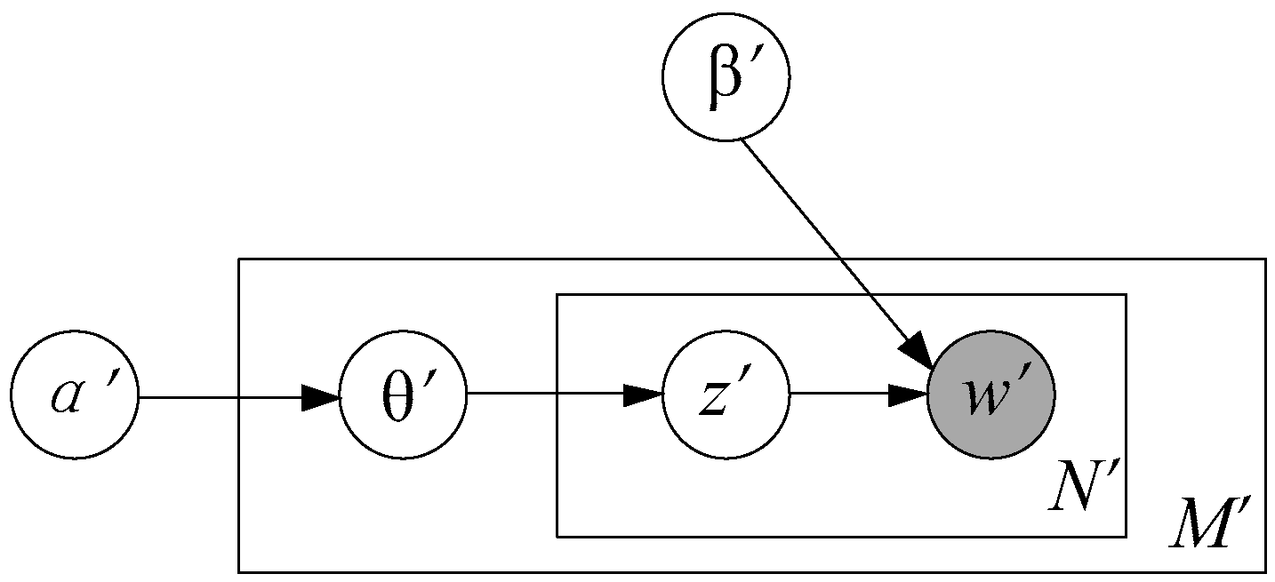
LDA model is a probabilistic graphical model that can be represented as a plate notation concisely in Figure 1. It can be logically divided into three levels: corpus level, document-level and word-level. The parameters α′ and β′ are corpus level parameters, which are sampled once in the process of generating a corpus. The random variable θ′ is a document level variable, which is sampled once for every document. The variables z′ and w′ are word level variables and are sampled once for each word in each document.
The basic idea of LDA is that documents are represented as random mixtures over latent topics, where each topic is characterized by a distribution over words [14]. The joint distribution of a topic mixture θ′, topic set z′, and word set w′ is given by
3.2. Problem Description
For remote sensing data retrieval, the staff usually submit their requirements for RS images to the image database system during their regular work, e.g., they gather SPOT-5 images that cover Shennongjia National Nature Reserve to carry out second class forestry resource inventory between May and June in every year. In other words, if a user frequently performs a certain task, he would be interested in RS images with particular parameters. To better interpret our model, we define some terms and notations used in this article. Table 1 lists the relevant notations.
Definition 1.
(Domain Task) Different application areas have different requirements on remote sensing data, e.g., forestry, agriculture, land resource and disaster. Taking forestry as an example, the common remote sensing data are Landset-5 data for first class forestry resource inventory, IKONOS and QuickBird data for second-class forestry resource inventory, and SPOT-5 data for woodland protection, utilization and planning. Users usually retrieve RS images from the database according to their current tasks. For professional users, the most common method of remote sensing data retrieval is to input specific parameter requirements into the system, such as time, spatial range and wavelength, while the domain tasks are not specifically stated in the query criteria. Therefore, a domain task z can be viewed as a latent topic.
Definition 2.
(Image Element) RS images are captured by relatively limited sensors, which have some fixed parameter configurations. In particular, the image parameters are usually fixed and consistent for a specific sensor. For example, image data captured by Thematic Mapper (TM) sensors contain seven bands (three in visible wavelengths and four in infrared) and two spatial resolutions (30 m and 120 m). The parameter requirements of remote sensing data depend on the domain task. Analogously to LDA, words are generated by topics in fixed conditional distributions, while image parameters are determined by the domain task. Take the second-class forestry resource inventory as an example. The specifications of remote sensing images are as follows: (1) A spatial resolution of less than 5 m is required. (2) The wavelength needs to contain the panchromatic and the near infrared bands (approximately 0.4–0.7 μm and 0.7–1.0 μm). (3) The data processing level is 2. For each task type, it might involve multiple specified images with different parameters. We take the image characteristics such as the spectral resolution, spatial resolution, and radiometric resolution as the words, and each of them is listed in the dictionary as a word. The sequence of the characteristics for each RS image, which is named image element e in our model, is a Nrv-dimension vector with erv = where Nrv is the number of image elements of the vth RS image that retrieved by the rth retrieval behavior (please refer to Definition 6).
Definition 3.
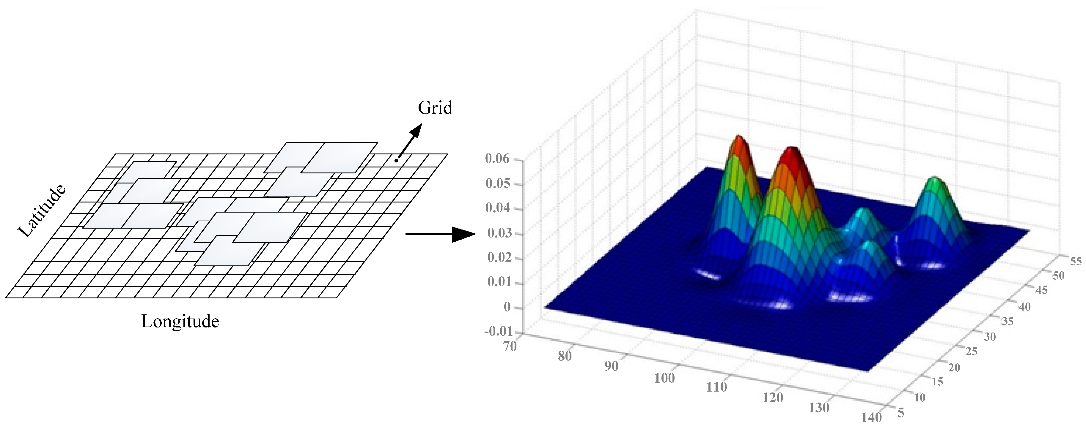
(Spatial Location) The tasks are directly related to actual land cover. Taking agriculture as an example, the relevant tasks are usually carried out in a region that is covered with crops, such as crop yield estimation, or disaster prevention [48]. Therefore, the distribution of spatial location preference depends more on the latent task and less on personal intuition. The spatial location can be extracted from the historical record of retrieval behavior and the RS image metadata. In order to transform the geographical space into one-dimensional space, the coverage area of RS images can be divided into grid cells based on a unified grid system (Figure 2). All grids are numbered or coded in accordance with certain rules, and each grid is listed in the dictionary as a word. Thus, a spatial location s is represented by a collection of grid cells that overlap with the image, which is a Srv-dimension vector with srv = where Srv is the number of grid cells of the vth RS image that retrieved by the rth retrieval behavior (please refer to Definition 6).
Definition 4.
(Time Preference) The time preference indicates the retrieval behavior of the user in the time dimension for each domain task. From the retrieval history record, a sequence of timestamps can be obtained according to the time at which the user accesses each image. For each specific task, the relevant timestamps are arranged in order, thus forming a time series, i.e., Qz = {t1, t2,…, tw}, where w is the indicator of timestamps in the time series for task z.
Definition 5.
(Time Period) There exist multiple time periods for the time series, since most domain tasks are periodic and a single user is assigned to multiple tasks. In the case above, the time period is one year, and forest pest monitoring is normally performed once a month, while forest fire warning is carried out once every 10 days. Therefore, the temporal features of the domain task should be represented by a periodic distribution, rather than a point-in-time, to reflect the real situation more precisely. For each latent task, the period T is extracted from the time series of task z.
Definition 6.
(Retrieval behavior) As shown in Figure 3, a retrieval behavior is generated based on the history of user actions and RS image metadata files (XML format). It consists of request time, user information, number of images, amount of data, and RS Image metadata (such as spatial locations, image parameters). In fact, a retrieval behavior can retrieve multiple images with different spatial location, image element and access time. So for a retrieval history record of a specific user, we create a retrieval behavior profile Dr, which is a set of triples (ev, sv, tv), that means the user accesses RS image v with spatial location sv and image element ev at time tv, The dataset D used in our model consists of retrieval behaviors of the user, i.e., D = {Dr: r ∈ [1,|D|]}, where |D| is the number of retrieval behavior profiles.
Remote sensing data are not as ubiquitous and random as items in location-based services, and the user groups are regular and professional users from relevant departments in the application fields. In a department, the domain tasks are basically similar, and the user retrieval behavior preferences of different users should be convergent. Therefore, we consider a department as a special large user, and all retrieval behavior profiles of the department as document set.
3.3. Space-Time Periodic Task Model
The LDA model is a generative model. It considers a document as a mixture of latent topics and chooses words in the item according to the topics. In our model, tasks are considered as the latent topics, and the image elements, timestamp and spatial location of the item are generated following a distribution specific to the chosen latent tasks in its corresponding period. The following section describes the generative process of our model. Based on the above definitions, we formalize our research problem as follows.
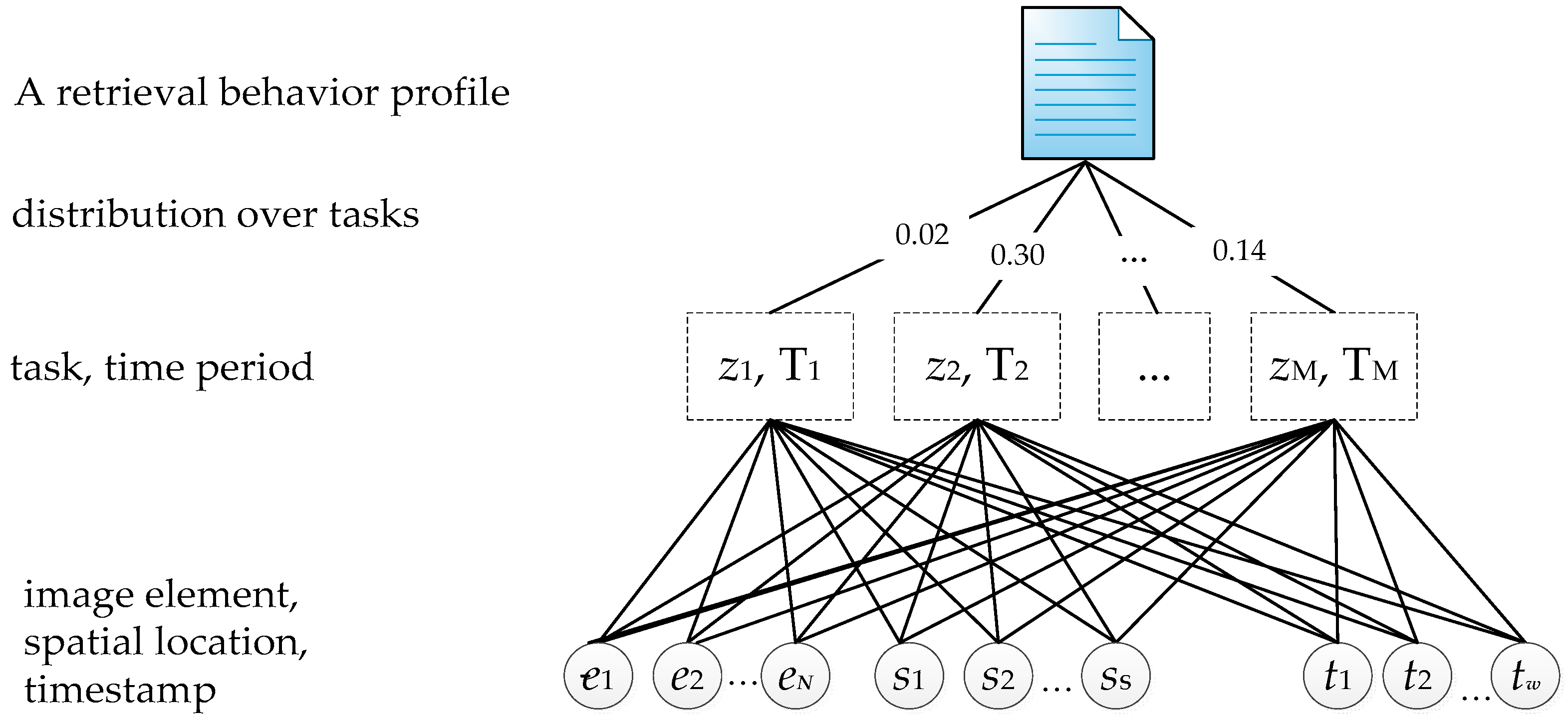
Given a set of image retrieval behavior documents D, the purpose is to model and learn the parameters of tasks, time, spatial location and image parameters for RS image recommendation. Figure 4 illustrates the components of a retrieval behavior document Dr. For each Dr, a task z is generated using some distributions of image element, spatial location and timestamp, and for each specific task z, a time period T can be extracted from the time series of the task z.
3.3.1. Model Structure
The proposed model is a probabilistic mixture generative model based on timestamp, spatial location and image characteristics, and the graphical model is shown in Figure 5. Spatial locations s, image elements e and timestamps t are modeled as observed random variables, shown as shaded circles, while the latent random variable z (tasks) is shown as unshaded circles. |D|, M denote the number of retrieval behavior documents and tasks, |V| represents the number of RS images which are included in each retrieval behavior and s, e represent the collection of spatial location grids and RS image elements for each RS image, not simply a single term in standard topic models. The user task z is associated with a multinomial distribution over the image elements e and spatial locations s, and a von Mises distribution over time t.
Noted that image element e is a collection of image characteristics, including the spectral resolution, spatial resolution, and radiometric resolution. The spatial location s is a collection of spatial grids with serial number, and each spatial grid has a hidden task label. Thus, in our model, ϕ is the probability parameter that individual spatial grid of each image belongs to the M tasks, which is a S × M matrix with . Similarly, the probability parameter σ that individual image elements of each image belong to the M tasks is a N × M matrix with . S, N are for the number of spatial grids and the number of image elements of all RS images that retrieved by retrieval behaviors, respectively.
In our model, the absolute time is mapped into a specific period. For each hidden task, there is a latent period T that would be extracted from the time series of the corresponding task. A major difference of our model is that it does not make Markov assumptions over state transition in time. In contrast to the topics over time (TOT, a non-Markov continuous-time model of topical trends) model [15], our model does not parameterize a continuous distribution over timestamps, as most common tasks have strong cyclical and seasonal characteristics. The von Mises distribution is applied to model the intensity distribution of task over time. This distribution is also known as the circularly distribution [49]. The normal von Mises distribution can be expressed as,
where Tz specifies the period of task z. τ is the initial phase point of task z, and κ is a measure of the concentration (a reciprocal measure of dispersion).When κ is zero, the von Mises distribution reduces to the uniform distribution. As κ increases, the distribution approaches a normal distribution. Thus, the probability distribution of time specific to tasks can be represented as P(t|κ, τ, T), which is determined by three parameters: T, κ, τ.
| Algorithm 1: Generative process |
| Input: a set of retrieval behavior documents D |
| Output: estimated parameters θ, ϕ, σ; |
| for each task z do |
| Draw ϕz ~ Dirichlet (β); |
| Draw σz ~ Dirichlet (γ); |
| Assign a task period Tz; |
| end for |
| for each retrieval behavior profile Dr do |
| Draw θr from Dirichlet (α); |
| Draw a task zri from multinomial zri ~ Multi(zri|θr); |
| Draw an image element ez from multinomial ez ~ Multi(e|σzri); |
| Draw a spatial grid sz from multinomial sz ~ Multi(s|ϕzri); |
| end for |
| for each task z do |
| for each period Tz do |
| Draw a timestamp tzw ~ P(t|κz, τz, Tz) from tzw ~ specific von Mises distribution; |
| end for |
| end for |
The generative process of STPT is outlined in Algorithm 1. To avoid overfitting, we place a Dirichlet prior parameter over each multinomial distribution. Thus, θ, ϕ, and σ are generated by Dirichlet distributions with parameters α, β, γ. The model discovers (1) latent user behavior preference distribution, θ; (2) task distribution over spatial grids, ϕ; (3) task distribution over image elements, σ. The generative model aims to capture the process of user behaviors for decision-making. For example, if a querying user wants to choose and download some RS images from database, he will choose the RS images based on the requirement of tasks. Task distributions θ model the latent user behavior preferences, from which the tasks are sampled. A task z is first chosen according to the task distribution θ, and then the selected task z in turn generates a period T, a relative time t mapped into T, a set of spatial grids s and relevant image elements e following on the generative distributions (i.e., ϕ and σ).
For each retrieval behavior document, the STPT model generates a task z using the multinomial distributions of the image element, spatial grid and von Mises distribution of timestamp of the image. The probability generative function can be defined with the joint distribution as follows:
where P(t|κ, τ, T) is the von Mises distribution given a specific task z, which is shown in Equation (2). The period T can be extracted from the time series of task z, which is discussed below.
3.3.2. Parameter Learning
The parameter learning of the STPT model can be divided into two major steps, normal parameter learning and time parameter learning, as shown in Figure 6. The normal parameter-learning step is to learn parameters by maximizing the marginal likelihood of the observed random variables s and e, and obtain the probability matrix of the elements and tasks, grids and tasks. Then each record is assigned to different tasks according to the probability distribution, and the time series of each task can be derived. The time parameter-learning step is to extract the period Tz from the time series for each specific task z and perform time parameter learning.
a. Normal Parameter Learning
There are two main methods to achieve the first step (normal parameter learning): Markov Chain Monte Carlo (MCMC) and Monte Carlo Exception Maximization (MCEM) [50]. Here, as one of MCMC methods, the collapsed Gibbs sampling algorithm is utilized to maximize the complete data likelihood, which is given in Equation (4).
As the sensitivity to hyper parameters is not very strong in our model, for simplicity, we use the fixed symmetric Dirichlet distribution (α = 50/M, β = γ = 0.1). In the sampling process, the next state is obtained by sequentially sampling all variables from their conditional distribution given all other variables. In the STPT model, we first sample the assignments of two variables (e and s) to task zri. According to the Bayesian rules, the conditional posterior distribution of zri is , where z¬ri denotes the assignment for all zrj such that j ≠ i. It can be computed based on the joint probability distribution as follows.
where nrz is the number of times that task z has been sampled from the multinomial distribution specific to the rth document Dr; nze is the number of times that image element e has been generated by task z. nzs is the number of times that spatial grid s has been generated by task z; the number n¬ri with superscript ¬ri denotes a quantity, excluding the current instance.
b. Time Parameter Learning
Given a specific task, a time subsequence is generated according to the time at which the user accesses each image. Although extracting the period from the whole time series is feasible, it will generate a lot of noisy data. To avoid this issue, the time series analysis and period extraction are performed on the time series of each specific task. Then, the periods of tasks are generated with Discrete Fourier Transformation (DFT) and spectral analysis. The detailed steps of the time period extraction algorithm are given in Algorithm 2. After processing, multiple obvious points with large amplitude might appear, and the largest one can be viewed as the period of the latent task.
| Algorithm 2: Period Extraction |
| input: time series for task z, Qz = {t1, t2, …, tw}; |
| output: the period Tz of task z; |
| step 1: Normalization |
| The time series is mapped to one dimension axis: according to the time at which the user accesses each image, the time items in the series are sorted by time intervals on the time axis, and the earliest point is taken as zero time. |
| Then computes the first order difference of Qz. |
| A new one series is obtained to denote Qz’ = {t’1, t’2, …, t’h} where h = w(w − 1)/2. |
| step 2: Discrete Fourier Transform |
| Perform Fourier transform on the new time series. |
| step 3: Spectral Analysis |
| Calculate spectral density using Equation (7). As it meets the frequency threshold, the period of time series is . |
| return the period value Tz at the spot of maximal Ak; |
Similarly, we also use a Gibbs sampling algorithm to perform the approximate inference of the von Mises distribution [51]. The posterior distribution is as follows:
where
where κ* and τ* are the updated parameters, and Tz is a constant value that can be extracted from the time subsequence corresponding to the specific task z. We introduce an impact factor λjp to represent the influence of other timestamps on the conditional distribution P(tp|t¬p, κp, τp), t¬p denotes all the timestamp elements of t except tp. Detailed derivation of Gibbs sampling for STPT is provided in Appendix A.
3.3.3. Inference Framework
This step addresses the problem of learning the parameters of the STPT model from data. Let (θ, σ, ϕ, κ, τ, T) be the parameters of the model to be learned. The inference process is shown in Algorithm 3. The algorithm contains three major parts. The first is to fetch tasks for each retrieval behavior document randomly; the second is to iterate and update parameters (θ, σ, ϕ) until convergence; the last is to extract the period Tz for each latent task using the Fourier transform method and to update the parameters (κ, τ) of the time distribution. Thus, for each task z, there is a von Mises distribution to associate with it.
| Algorithm 3: Inference Framework of STPT model |
| input: user retrieval behavior document D, Limitation of Iteration Npl, Priors α, β, γ; |
| output: estimated parameter θ, ϕ, σ and {κz, τz}; |
| for each document Dr ∈ D do |
| Assign task randomly; |
| end for |
| Initialize task mode parameters θ, ϕ and σ; |
| for iteration = 1 to Npl do |
| for each document Dr ∈ D do |
| Update task assignment using Equation (5); |
| Update model parameter θrz, ϕzs and σze as follows |
| end for |
| end for |
| for each task z do |
| Fetch the time series Qz and extracted the period Tz with Algorithm 2; |
| Initialize the κz and τz; |
| for iteration = 1 to Npl do |
| for each item <e, s, t> ∈ z do |
| Update parameters κz and τz using Equation (8); |
| end for |
| end for |
| end for |
| Return estimated model parameters θ, ϕ, σ and {κz, τz}; |
4. Experimental Evaluations
In this section, we have implemented the Gibbs sampler and the parameter learning algorithm for the STPT model and performed experiments using both synthetic and real data. The accuracy and effectiveness of our model were evaluated by comparing with the results of existing approaches.
4.1. Dataset
Geographic Information Metadata ISO 19115-1:2014 (International Standards Organization, 2003) is taken as a reference to generate the satellite image metadata, which are described with XML. There are seven kinds of metadata information, including image identity, image file, image acquisition, latitude and longitude, spatial reference, product quality and release [52]. Here, image acquisition information involves some sensor information, such as platform, sensor type, sensor name, band information, and orbit number of the image. To ensure the quality of the simulated data, the values of the main characteristics in the metadata comply with the requirements of common satellite remote sensing data types, such as Landsat, CBERS, SPOT5/HRG, IKONOS, NOAA/AVHRR, QuickBird, GeoEye-1, and WorldView.
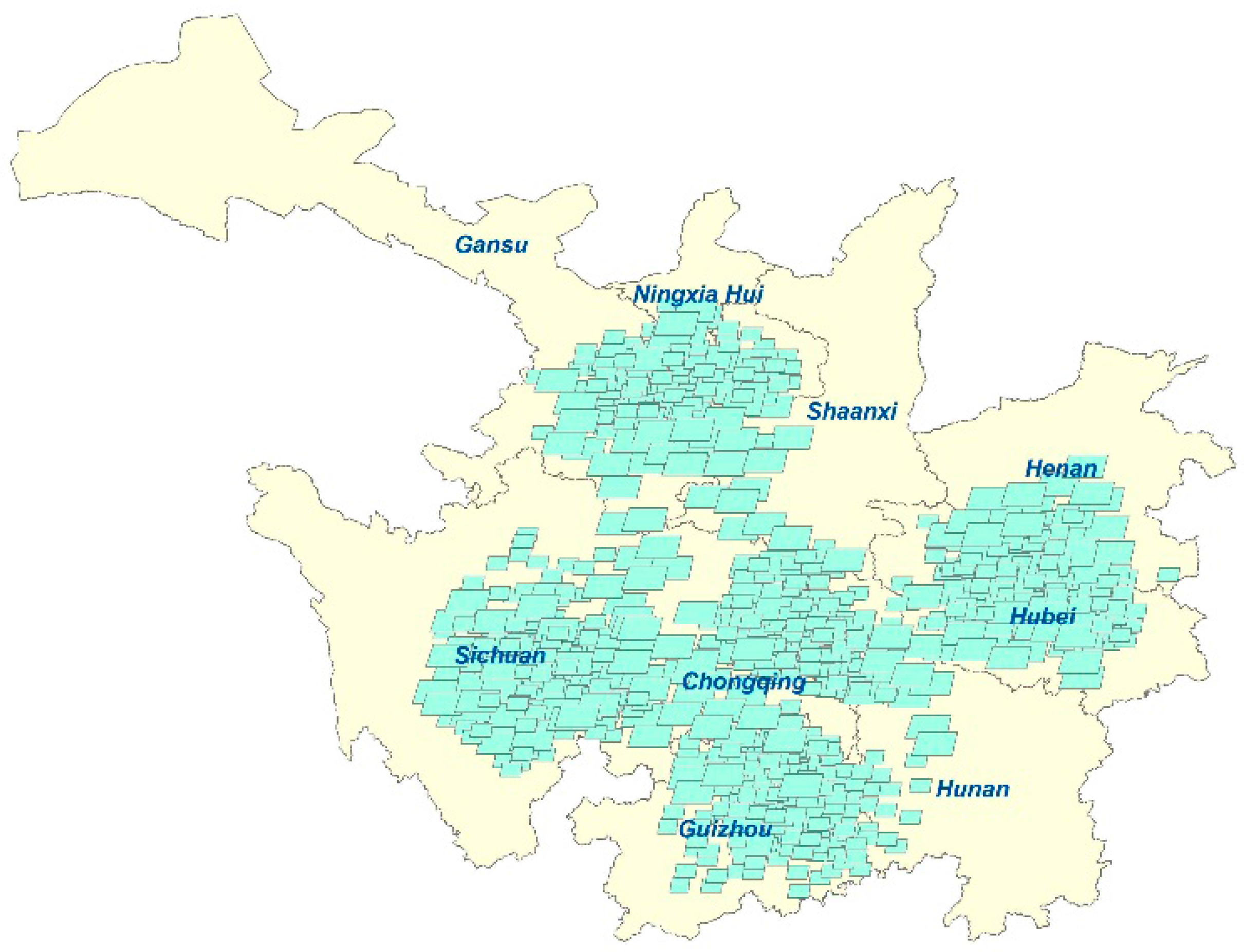
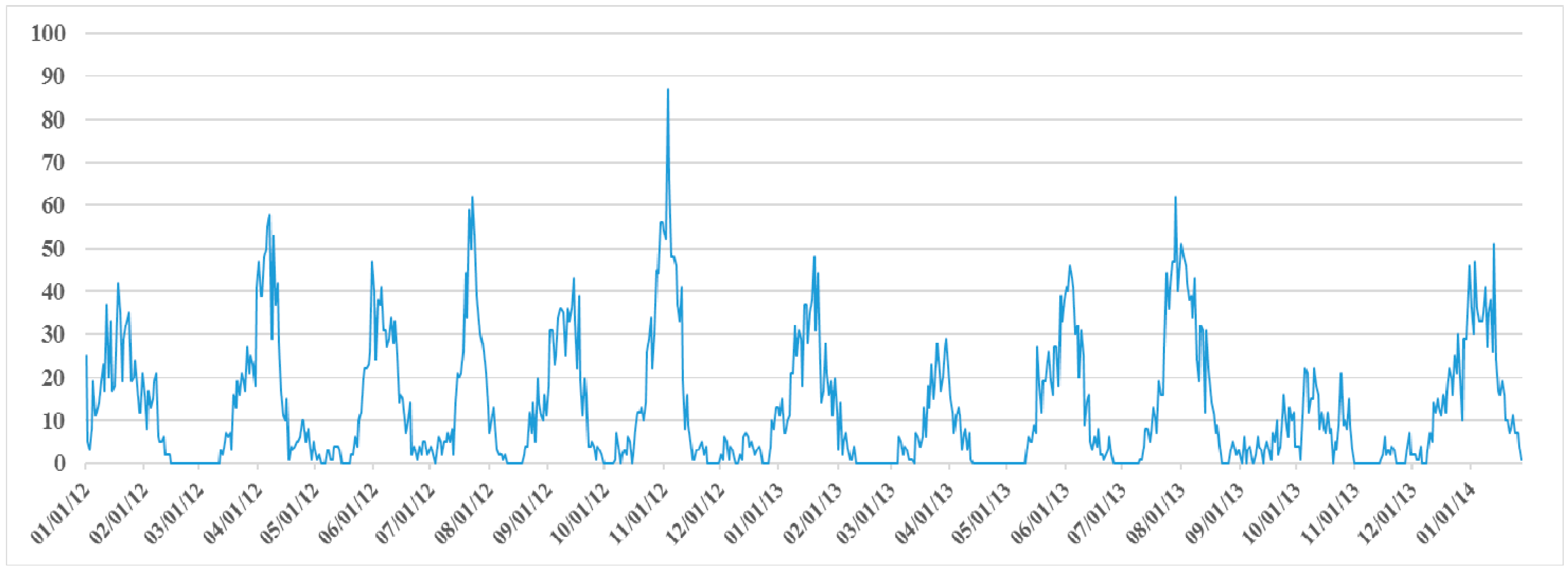
We extracted user searching behaviors from a department between January 2012 and January 2014, and obtained valid retrieval records that involved 9790 image data items from the semantic-based RS image retrieval prototype system [53]. These remote sensing data are distributed mainly over eight provinces in China: Ningxia, Shanxi, Sichuan, Chongqing, Henan, Hubei and Guizhou, shown in Figure 7. Figure 8 displays the number of requests per day during this time, and the time distribution rarely exhibits a fixed period pattern since it may involve multiple domain tasks.
4.2. Comparison Approaches
In our experiment, we compare the performance of our STPT model with those of the following methods, which can be applied to the space-time recommendation system.
Item Location-Aware Topic (ILA-LDA). ILA-LDA, proposed in [44], is a location-aware probabilistic generative model that exploits location-based ratings to model user profiles and produce recommendations. To ensure that this model is effective on the above dataset, we use a fixed value as the item normal score (score = 1). Note that this model does not take the temporal patterns into account.
Topic over Time (TOT). TOT is a temporal topic model that explicitly models time jointly with word co-occurrence patterns [15]. It uses the continuous Beta distribution over time instead of discretizing time.
Spatio-Temporal Topic (STT). The STT model was developed to capture the spatial and temporal aspects of user check-ins in a single probabilistic model [16]. User profiles can be modeled by exploiting the interdependence between temporal activity patterns and locations.
Space-Time Periodic Task (STPT). STPT is the spatiotemporal periodic task model that was proposed in Section 3. It takes the periodicity of the task into account and predicts task distributions over time and location.
4.3. Experimental Evaluations
We use k-fold Cross-validation to evaluate the recommendation models. The original sample is randomly partitioned into 10 equally sized subsamples. Of the 10 subsamples, the 9 subsamples are used as training data, and the remaining single subsample is retained as the validation data for testing the models. For the specific user, the system will recommend the top-k images according to the individual user behavior profile. The initialization parameters of STPT are set to default values (α = 50/K, β = 0.1, γ = 0.1, κ= 2, and M = 20), and updated with training data according to Algorithms 2 and 3. Finally, given a batch of new RS images, the STPT model can calculate several probabilities P(e, t, s) for the specific user. Then the items in the recommendation list are ranked according to the probability that the user will request the image at time t with image characteristic e and spatial location s. It can be calculated with the following Equation (15):
Normalized Discounted Cumulative Gain (NDCG) is employed to evaluate the effectiveness of the proposed method [54]. NDCG is a popular and well-known measurement that is applied in information retrieval. A higher NDCG value indicates that the highly relevant items appeared in the result list. NDCG@k is used to measure the relevance of the top-k items, as shown in Equation (16).
where k is the number of recommended items. reli is the relevance score of the items, and {Ii−n} indicates the RS image dataset that user needs at ith day to come, and m is the time span (days) of ranking list. IDCGk indicates the DCGk value of ideal ranking list. The evaluation procedure is as follows:
- (1)
- Generate randomly a batch dataset from the remaining single subsample as test case |Stest|.
- (2)
- For each RS image, compute the probability P(e, t, s) with the STPT model, and generate a top-k recommendation list RSISTPT based on P(e, t, s).
- (3)
- Given the relevance scores of RSISTPT, generate the ideal ranking list RSIGT which is the ground truth list. In addition, calculate the NDCG@k using Equation (16).
4.3.1. Top-k Recommendation
We collected all historical data for a specific user, “F00019@D01” (D01 stands for a department). This data set is composed of 9790 items of image metadata, and is split into testing and training data sets based on 10-fold cross-validation. Note that the time series of the RS image list in each subsample is continuous. Then, we specified the initialization parameters of the models (α = 50/M, β = 0.1 and γ = 0.1), the number of latent tasks (M = 20), and the spatial granularity (5 km × 5 km).
Figure 9 shows the performances of the recommendation algorithms with 7 days, 14 days and 30 days as the time slices. As demonstrated above, the time slice indicates the valid time span for measuring the RS image list. When we set the time slice to 7 days, the recommendation model generates a list of predictive items that user might require in the next 7 days. Within the time span (7 days), if there are images both in predictive item list and the test item list, the recommendation result is regarded as correct. As a result, the precisions of the model would be calculated by comparing with the test data. Theoretically, on the one hand, the longer the time span is, the more accurate the recommendation model will be (Figure 9d). On the other hand, if the time span is too long, the recommendation result will be meaningless. For each test set, we ensure that the number of available candidate items is larger than k within each time slice. In Figure 9, when the number of Top-k items is greater than 20, the performances of the model stabilize, and our model has obvious advantages over the other models. According to the result, we observed that: (1) the proposed model performs best and the STT model performs better than ILA-LDA and TOT since STPT and STT exploit the temporal and spatial preferences; (2) the ILA-LDA model has relatively poor performance because it does not take into account the distribution of user preferences over time; (3) TOT is inferior to STT and STPT since it lacks spatial location consideration. Also, in the TOT model, the time distribution of each topic is described as a Beta distribution, which is not suitable for the time prediction of the short cycle topic.
4.3.2. Effect of Spatial Granularity and Number of Tasks
The performances of the models are usually affected by inexperienced parameters, such as the number of tasks and the granularity of spatial location. Compared to the variety of words in document data sets, the type of RS images is limited and fixed, so the number of latent tasks is smaller. The latent tasks in our model are composed of timestamps, image elements and spatial grids, by which the spatial area of user interest is partitioned into many grids. The number of tasks is associated with the granularity of spatial location, and this has an impact on performance. We designed an experiment to study the effect of the number of tasks and the granularity of spatial location.
a. Effect of Spatial Granularity
Figure 10 shows the recommendation accuracy (NDCG@25) of models with different granularities of spatial location. Although the NDCG@25 of STPT is lower than that of STT when the grid size is 10 km, STPT is superior to other models in terms of overall performance. The results obviously show that the models obtain the optimal effect when grid size equals 5 km. The NDCG@25 of TOT is fixed since this model does not consider spatial features.
In theory, the greater the grid size is, the more difficult it is to identify the area of interest. The overall performance of a recommendation model with finer granularity is better than that with coarser granularity. In fact, the accuracy values of models decrease as the granularity becomes finer (1 km × 1 km). The reason is that overly fine granularity results in the spatial distribution of the user preference becoming flat and decentralized, and reduces the effect of spatial location.
b. Influence of the Number of Tasks
After tuning the performances of the models in terms of spatial granularity, it is determined that the best grid size is 5 km. The number of tasks is also a critical factor affecting the performance of the model. Next, we determine the influence of the number of tasks on the recommendation models. Setting the grid size to 5 km, the results show that as the number of tasks increases, the accuracy values of the recommendation models first increase, and then decrease. However, for each model, the optimum efficiency is not attained at the same point with the same number of tasks in Figure 11. The optimal number of tasks is 15 for the ILA-LDA model, 25 for the TOT model, and 20 for both the STT and STPT models.
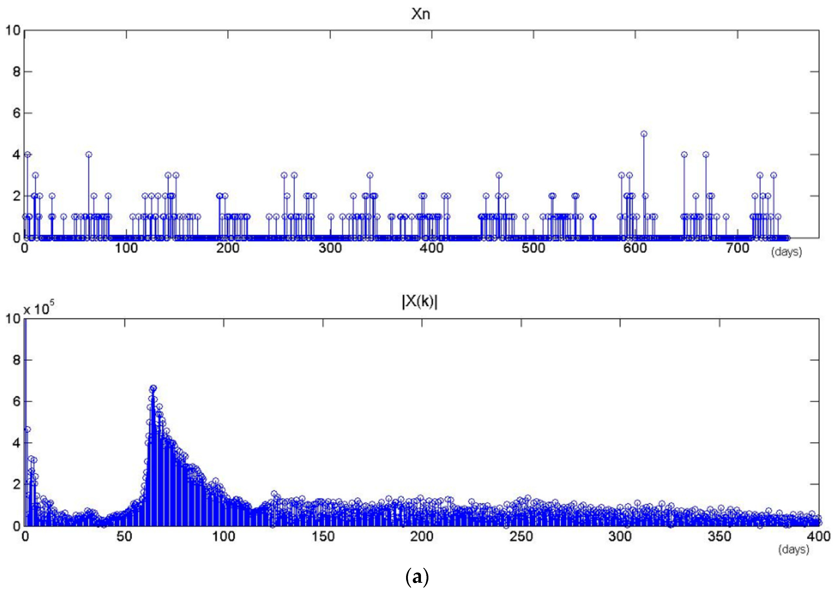
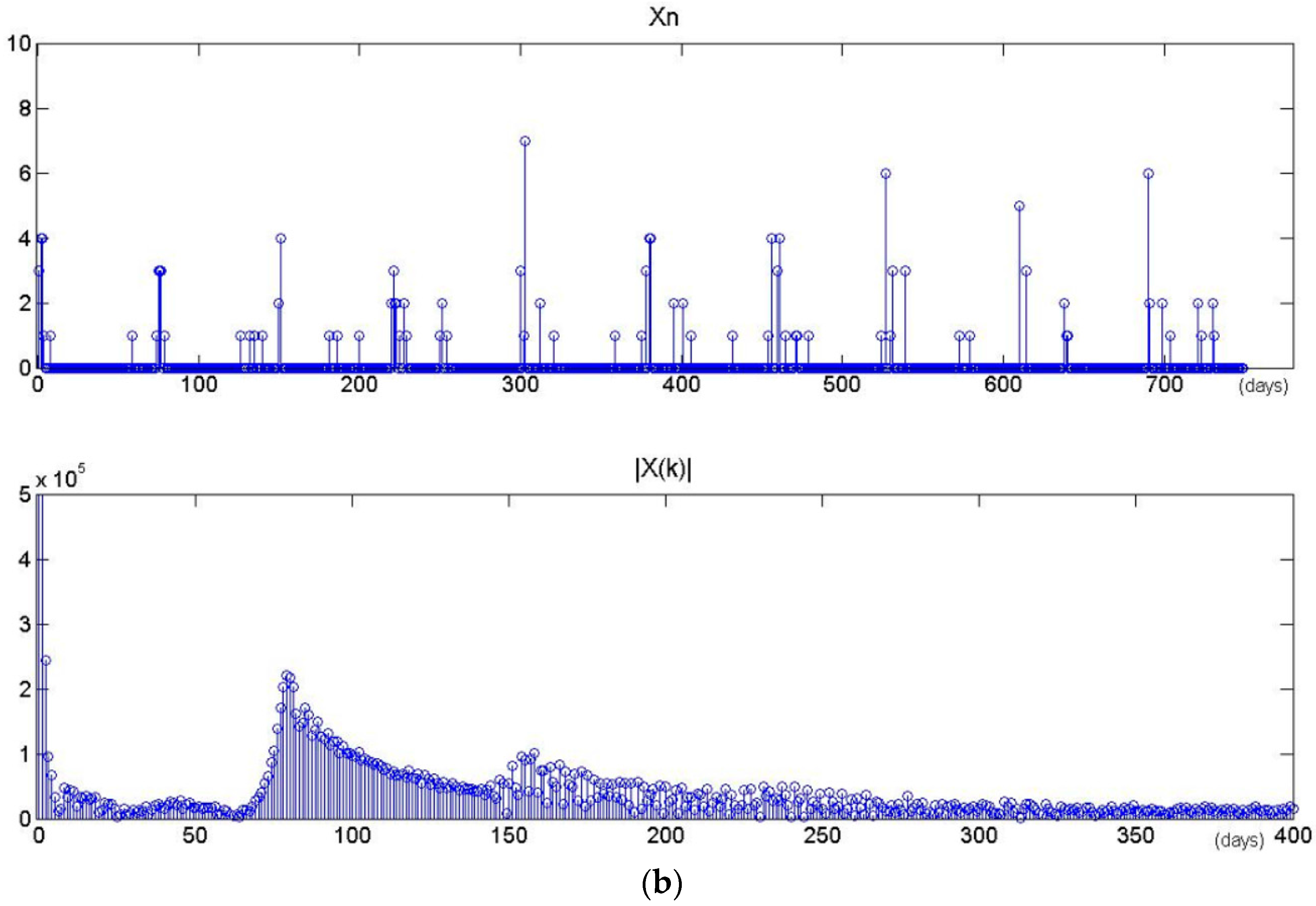
The proposed model assigns a period for each latent task. Consequently, the time series will become sparse as the number of tasks increases. Figure 12 shows the results of period extractions for two latent tasks that are chosen randomly from the STPT model with different number of tasks (M = 20 and M = 40). Xn is the time sequence of specific task z. |Xk| is the result of DFT and spectral analysis. Their maximum amplitudes of |Xk| are located in 65-days and 79-days respectively, which may serve as the periods of the tasks. In all training data, there are 398 timestamps belonging to each task on average when the number of tasks is set to 20, and only 178 timestamps belonging to each task when the number of tasks is set to 40. Figure 13 shows the probability distributions of specific tasks over time presented in Figure 12. We observe that a dense timestamp will generate a reliable period value and has a high fitting degree. The period is not significant when the time series is sparse. Therefore, the number of tasks will impact the performance by influencing the time period as well as the spatial location.
4.3.3. Training and Online Recommendation Time
The proposed model is not an online and incremental learning model. In the short term, the domain task is relatively stable and the parameter requirements of RS images are also fixed for specific task, therefore, there will be fewer changes in the user preference. Meanwhile, the time preference is also dependent on task. So the STPT model would be retrained after a period of time (e.g., three months, half year).
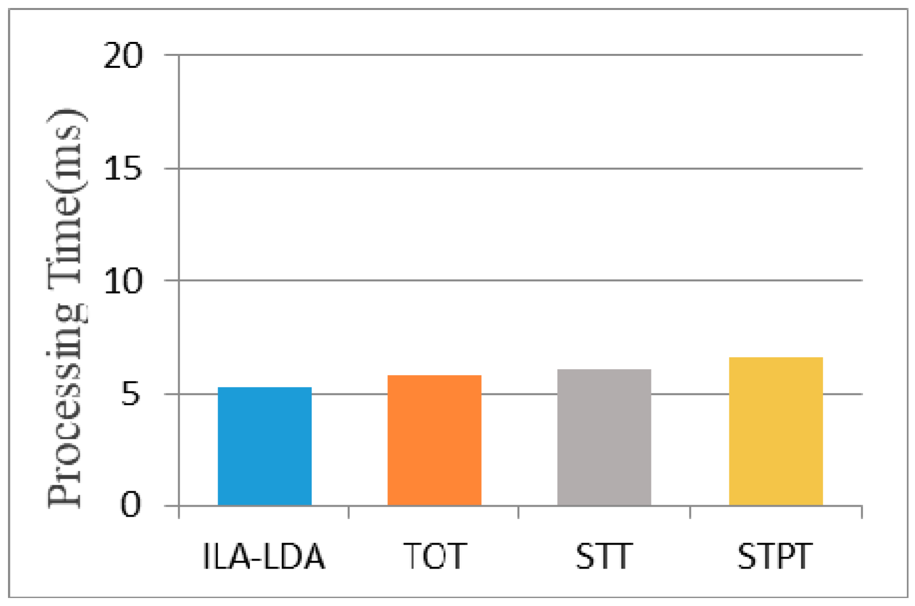
Now we make simple analysis of the effects of offline training and online recommendation time. All recommendation algorithms were implemented in the MATLAB platform on a PC running Windows 7 with four Intel Core i5-3470 processors and 32 GB memory. In the experiment, the time cost of STPT is within 4 h 25 min in terms of 9790 image metadata, 398 timestamps, 20 tasks, and 5 km grid size. TOT and STT cost 3 h 15 min and 3 h 55 min, respectively. Just in terms of results, the time cost of STPT is a little higher than TOT and STT. However, that is due to many factors are considered in developing our model, such as the Gibbs sampling method used for performing the parameter learning and time period extraction, and 10-fold Cross-validation used for splitting into testing and training data set. Figure 14 present the average online efficiency of different approaches to generate the recommendations for the queries for RS images. As the figure shows, there is little difference in online recommendation efficiency. The proposed model also can produce faster responses to queries once model parameters are learned.
5. Conclusions
In this paper, we present a recommendation model for building reliable profiles by using retrieval history records and unstructured meta-data of RS image data. We show how to incorporate the space and time features into the topic model and build the spatiotemporal periodic task model. We map both the spatial location and image characteristics to the latent topic model, and are able to build a single time distribution for each latent task due to the stability and periodicity of tasks. In the process of parameter learning, we first perform the parameter learning only for space and image characteristics with the Gibbs sampling method, and then extract the corresponding period and recalculate the model parameters. We demonstrate the usefulness of the STPT model by comparing it with the existing models. The results of the experiment show that our model outperforms ILA-LDA, TOT and STT in terms of the NCDG score of the top-k recommendations. Furthermore, we also discuss the influences of the granularity of spatial location and the number of latent tasks on top-k recommendation.
There are several important avenues for future work. First, we would like to address the cold-start problem by utilizing the domain knowledge. The model can recommend image data to new users according to the preferences of other users in the same sector. New items can be recommended to users by computing the similarity between the existing items and the new ones. Second, the period can be taken as an updated parameter so that the model can avoid recomputing the parameters, thereby enhancing the efficiency.
Acknowledgments
The authors would like to acknowledge the support and contribution of the National Key Research and Development Program of China (No. 2017YFB0503502, 2017YFB0503601) and the Fundamental Research Funds for the Central Universities (No. 7771705). Thanks are due to Di Chen for assistance with the experiments and to Jiping Liu for excellent technical support.
Author Contributions
Xiuhong Zhang, Di Chen and Jiping Liu contributed to the conception of the study; Xiuhong Zhang and Di Chen performed the data analyses and wrote the manuscript; Jiping Liu contributed the central idea and helped perform the analysis with constructive discussions.
Conflicts of Interest
The authors declare no conflict of interest.
Appendix A
Gibbs Sampling Derivation for STPT
The von Mises distribution is applied to model the intensity distribution of task over time. This distribution is also known as the circularly distribution [51]. The joint probability density function of the von Mises distribution for task z as follows:
where Tz specifies the period of task z. τ is the initial phase point of task z, and κ is a measure of concentration.
As shown in [51], the von Mises conditionals are univariate von Mises distributions, and Gibbs sampling algorithm is suitable to perform the approximate inference of the von Mises distribution. The posterior distribution is as follows:
Let = v, then the posterior distribution can becomes
can be considered as the form of “acosx+bsinx”, then we can get:
Now define the updated parameters and by
and substitute these expressions into Equations (A3) and (A4). Then we have
and then substitute = v into and , we can get
We introduce an impact factor λip to represent that the conditional distribution P(tp|t¬p, κp, τp) is influenced by other timestamps. Let
References
- Fang, C.Y.; Lin, H.; Xu, Q.; Tang, D.L.; Wang, W.C.; Zhang, J.X.; Pang, Y.C. Online generation and dissemination of disaster information based on satellite remote sensing data. In Proceedings of the Web and Wireless Geographical Information Systems, Shanghai, China, 11–12 December 2008; pp. 63–74. [Google Scholar]
- Campbell, J.B.; Wynne, R.H. Introduction to Remote Sensing; Guilford Press: New York, NY, USA, 2011. [Google Scholar]
- Singh, A. Review article digital change detection techniques using remotely-sensed data. Int. J. Remote Sens. 1989, 10, 989–1003. [Google Scholar] [CrossRef]
- Ma, Y.; Wang, L.; Liu, P.; Ranjan, R. Towards building a data-intensive index for big data computing—A case study of Remote Sensing data processing. Inf. Sci. 2015, 319, 171–188. [Google Scholar] [CrossRef]
- Wu, L.; Liu, L.; Li, J.; Li, Z. Modeling user multiple interests by an improved GCS approach. Expert Syst. Appl. 2005, 29, 757–767. [Google Scholar]
- Ferecatu, M.; Boujemaa, N. Interactive remote-sensing image retrieval using active relevance feedback. IEEE Trans. Geosci. Remote Sens. 2007, 45, 818–826. [Google Scholar] [CrossRef]
- Roy, D.P.; Trigg, S.; Bhima, R.; Brockett, B.H.; Dube, O.P.; Frost, P.; Govender, N.; Le Roux, J.; Neo-Mahupeleng, G.; Norman, M. Utility of satellite fire product accuracy information—Perspectives and recommendations from the Southern Africa fire network. IEEE Trans. Geosci. Remote Sens. 2006, 44, 1928–1930. [Google Scholar] [CrossRef]
- Matyas, C.; Schlieder, C. A spatial user similarity measure for geographic recommender systems. In GeoSpatial Semantics; Springer: New York, NY, USA, 2009; pp. 122–139. [Google Scholar]
- Ivánová, I.; Morales, J.; de By, R.; Beshe, T.; Gebresilassie, M. Searching for spatial data resources by fitness for use. J. Spat. Sci. 2013, 58, 15–28. [Google Scholar] [CrossRef]
- Beshe, T. Turning Spatial Data Search Engine to Spatial Data Recommendation Engine. Master’s Thesis, University of Twente, Enschede, The Netherlands, 2012. [Google Scholar]
- O’Sullivan, D.; McLoughlin, E.; Bertolotto, M.; Wilson, D. Adaptive presentation and navigation for geospatial imagery tasks. In Proceedings of the Adaptive Hypermedia and Adaptive Web-Based Systems, Eindhoven, The Netherlands, 23–26 August 2004; pp. 688–698. [Google Scholar]
- Wilson, D.C.; Bertolotto, M.; McLoughlin, E.; O’Sullivan, D. Knowledge capture and reuse for geo-spatial imagery tasks. In Proceedings of the 5th International Conference on Case-Based Reasoning: Research and Development, Trondheim, Norway, 23–26 June 2003; pp. 622–636. [Google Scholar]
- McLoughlin, E.; O Sullivan, D.; Bertolotto, M.; Wilson, D. A knowledge management system for intelligent retrieval of geo-spatial imagery. Lect. Notes Comput. Sci. 2004, 535–544. [Google Scholar]
- Blei, D.M.; Ng, A.Y.; Jordan, M.I. Latent dirichlet allocation. J. Mach. Learn. Res. 2003, 3, 993–1022. [Google Scholar]
- Wang, X.; McCallum, A. Topics over time: A non-Markov continuous-time model of topical trends. In Proceedings of the 12th ACM SIGKDD International Conference on Knowledge Discovery and Data Mining, Philadelphia, PA, USA, 20–23 August 2006; pp. 424–433. [Google Scholar]
- Bo, H.; Jamali, M.; Ester, M. Spatio-Temporal Topic Modeling in Mobile Social Media for Location Recommendation. In Proceedings of the 2013 IEEE 13th International Conference on Data Mining (ICDM), Dallas, TX, USA, 7–10 December 2013; pp. 1073–1078. [Google Scholar]
- Xia, Y.; Zhu, X.; Li, D.; Zhan, Q. A user profile model for intelligent delivery of spatial information. In Proceedings of the Geoinformatics 2008 and Joint Conference on GIS and Built Environment: Geo-Simulation and Virtual GIS Environments, Guangzhou, China, 28–29 June 2008. [Google Scholar]
- Sarwar, B.; Karypis, G.; Konstan, J.; Riedl, J. Item-based collaborative filtering recommendation algorithms. In Proceedings of the 10th International Conference on World Wide Web, Hong Kong, China, 1–5 May 2001; pp. 285–295. [Google Scholar]
- Schafer, J.B.; Konstan, J.A.; Riedl, J. E-commerce recommendation applications. In Applications of Data Mining to Electronic Commerce; Springer: New York, NY, USA, 2001; pp. 115–153. [Google Scholar]
- Pirasteh, P.; Jung, J.J.; Hwang, D. Item-Based Collaborative Filtering with Attribute Correlation: A Case Study on Movie Recommendation; Springer: New York, NY, USA, 2014; pp. 245–252. [Google Scholar]
- Xia, J.B. E-Commerce Product Recommendation Method Based on Collaborative Filtering Technology. In Proceedings of the International Conference on Smart Grid and Electrical Automation, Zhangjiajie, China, 11–12 August 2016. [Google Scholar]
- Foster, J. Collaborative information seeking and retrieval. Ann. Rev. Inf. Sci. Technol. 2006, 40, 329–356. [Google Scholar] [CrossRef]
- Rebollo-Monedero, D.; Forné, J.; Solanas, A.; Martínez-Ballesté, A. Private location-based information retrieval through user collaboration. Comput. Commun. 2010, 33, 762–774. [Google Scholar] [CrossRef] [Green Version]
- Bellogín, A.; Wang, J.; Castells, P. Text Retrieval Methods for Item Ranking in Collaborative Filtering. In Proceedings of the European Conference on Advances in Information Retrieval, Dublin, Ireland, 18–21 April 2011; pp. 301–306. [Google Scholar]
- Melville, P.; Mooney, R.J.; Nagarajan, R. Content-boosted collaborative filtering for improved recommendations. In Proceedings of the Eighteenth National Conference on Artificial Intelligence, Edmonton, AB, Canada, 28 July–1 August 2002; pp. 187–192. [Google Scholar]
- Barragáns-Martínez, A.B.; Costa-Montenegro, E.; Burguillo, J.C.; Rey-López, M.; Mikic-Fonte, F.A.; Peleteiro, A. A hybrid content-based and item-based collaborative filtering approach to recommend TV programs enhanced with singular value decomposition. Inf. Sci. 2010, 180, 4290–4311. [Google Scholar] [CrossRef]
- Yao, L.; Sheng, Q.Z.; Ngu, A.H.H.; Yu, J. Unified Collaborative and Content-Based Web Service Recommendation. IEEE Trans. Serv. Comput. 2015, 8, 453–466. [Google Scholar] [CrossRef]
- Mathew, P.; Kuriakose, B.; Hegde, V. Book Recommendation System through content based and collaborative filtering method. In Proceedings of the International Conference on Data Mining and Advanced Computing, Ernakulam, India, 16–18 March 2016; pp. 47–52. [Google Scholar]
- Lee, B.-H.; Kim, H.-N.; Jung, J.-G.; Jo, G. Location-based service with context data for a restaurant recommendation. In Proceedings of the Database and Expert Systems Applications, Kraków, Poland, 4–8 September 2006; pp. 430–438. [Google Scholar]
- Gupta, G.; Lee, W.C. Collaborative Spatial Object Recommendation in Location Based Services. In Proceedings of the 39th International Conference on Parallel Processing Workshops, San Diego, CA, USA, 13–16 September 2010; pp. 24–33. [Google Scholar]
- Wang, H.; Terrovitis, M.; Mamoulis, N. Location recommendation in location-based social networks using user check-in data. In Proceedings of the ACM Sigspatial International Conference on Advances in Geographic Information Systems, Orlando, FL, USA, 5–8 November 2013; pp. 374–383. [Google Scholar]
- Li, H.; Hong, R.; Zhu, S.; Ge, Y. Point-of-Interest Recommender Systems: A Separate-Space Perspective. In Proceedings of the IEEE International Conference on Data Mining, Atlantic City, NJ, USA, 14–17 November 2015; pp. 231–240. [Google Scholar]
- Kosmides, P.; Demestichas, K.; Adamopoulou, E.; Remoundou, C.; Loumiotis, I.; Theologou, M.; Anagnostou, M. Providing recommendations on location-based social networks. J. Ambient Intell. Humaniz. Comput. 2016, 7, 1–12. [Google Scholar] [CrossRef]
- Wang, W.; Yin, H.; Sadiq, S.; Chen, L.; Xie, M.; Zhou, X. SPORE: A sequential personalized spatial item recommender system. In Proceedings of the IEEE 32nd International Conference on Data Engineering, Helsinki, Finland, 16–20 May 2016; pp. 954–965. [Google Scholar]
- Yin, H.; Cui, B.; Sun, Y.; Hu, Z.; Chen, L. LCARS: A spatial item recommender system. ACM Trans. Inf. Syst. 2014, 32, 11. [Google Scholar] [CrossRef]
- Wang, W.; Yin, H.; Chen, L.; Sun, Y.; Sadiq, S.; Zhou, X. Geo-SAGE: A Geographical Sparse Additive Generative Model for Spatial Item Recommendation. In Proceedings of the 21th ACM SIGKDD International Conference on Knowledge Discovery and Data Mining, Sydney, NSW, Australia, 10–13 August 2015; pp. 1255–1264. [Google Scholar]
- Oku, K.; Kotera, R.; Sumiya, K. Geographical recommender system based on interaction between map operation and category selection. In Proceedings of the 1st International Workshop on Information Heterogeneity and Fusion in Recommender Systems, Barcelona, Spain, 26–30 September 2010; pp. 71–74. [Google Scholar]
- Hong, J.-H.; Su, Z.L.-T.; Lu, E.H.-C. A recommendation framework for remote sensing images by spatial relation analysis. J. Syst. Softw. 2014, 90, 151–166. [Google Scholar] [CrossRef]
- Zhang, J.D.; Chow, C.Y. CoRe: Exploiting the personalized influence of two-dimensional geographic coordinates for location recommendations. Inf. Sci. 2015, 293, 163–181. [Google Scholar] [CrossRef]
- Krestel, R.; Fankhauser, P.; Nejdl, W. Latent dirichlet allocation for tag recommendation. In Proceedings of the Third ACM Conference on Recommender Systems, New York, New York, USA, 23–25 October 2009; pp. 61–68. [Google Scholar]
- Guo, Y.; Joshi, J.B.D. Topic-based personalized recommendation for collaborative tagging system. In Proceedings of the 21st ACM Conference on Hypertext and Hypermedia, Toronto, ON, Canada, 13–16 June 2010; pp. 61–66. [Google Scholar]
- Hong, L.; Ahmed, A.; Gurumurthy, S.; Smola, A.J.; Tsioutsiouliklis, K. Discovering geographical topics in the twitter stream. In Proceedings of the 21st International Conference on World Wide Web, Lyon, France, 16–20 April 2012; pp. 769–778. [Google Scholar]
- Ference, G.; Ye, M.; Lee, W.C. Location recommendation for out-of-town users in location-based social networks. In Proceedings of the ACM International Conference on Information & Knowledge Management, San Francisco, CA, USA, 27 October–1 November 2013; pp. 721–726. [Google Scholar]
- Yin, H.; Cui, B.; Chen, L.; Hu, Z.; Zhang, C. Modeling Location-Based User Rating Profiles for Personalized Recommendation. ACM Trans. Knowl. Discov. Data 2015, 9, 1–41. [Google Scholar] [CrossRef]
- Yuan, Q.; Cong, G.; Ma, Z.; Sun, A.; Thalmann, N.M. Time-aware point-of-interest recommendation. In Proceedings of the 36th International ACM SIGIR Conference on Research and Development in Information Retrieval, Dublin, Ireland, 28 July–1 August 2013; pp. 363–372. [Google Scholar]
- Zhang, J.D.; Chow, C.Y. Spatiotemporal Sequential Influence Modeling for Location Recommendations: A Gravity-based Approach. ACM Trans. Intell. Syst. Technol. 2015, 7, 1–25. [Google Scholar] [CrossRef]
- Zhang, J.D.; Chow, C.Y. Point-of-interest recommendations in location-based social networks. Sigspat. Spec. 2016, 7, 26–33. [Google Scholar] [CrossRef]
- Oetter, D.R.; Cohen, W.B.; Berterretche, M.; Maiersperger, T.K.; Kennedy, R.E. Land cover mapping in an agricultural setting using multiseasonal Thematic Mapper data. Remote Sens. Environ. 2001, 76, 139–155. [Google Scholar] [CrossRef]
- Hughes, G. Multivariate and Time Series Models for Circular Data with Applications to Protein Conformational Angles. Ph.D. Thesis, University of Leeds, Leeds, UK, 2007. [Google Scholar]
- Levine, R.A.; Casella, G. Implementations of the Monte Carlo EM algorithm. J. Comput. Graph. Stat. 2001, 10, 422–439. [Google Scholar] [CrossRef]
- Razavian, N.S.; Kamisetty, H.; Langmead, C.J. The Von Mises Graphical Model: Structure Learning. Carnegie Mellon University School of Computer Science Technical Report; Carnegie Mellon University: Pittsburgh, PA, USA, 2011. [Google Scholar]
- Li, Q.; Wang, S.; Chen, B. Remote sensing image distribute system supported by metadata. In Proceedings of the 2005 IEEE International Geoscience and Remote Sensing Symposium, Seoul, Korea, 25–29 July 2005; p. 4. [Google Scholar]
- Zhu, X.; Li, M.; Guo, W.; Zhang, X. Semantic-based user demand modeling for remote sensing images retrieval. In Proceedings of the 2012 IEEE International Geoscience and Remote Sensing Symposium (IGARSS), Munich, Germany, 22–27 July 2012; pp. 2902–2905. [Google Scholar]
- Manning, C.D.; Raghavan, P.; Schütze, H. Introduction to Information Retrieval: Boolean Retrieval; Cambridge University Press: Cambridge, UK, 2008; pp. 824–825. [Google Scholar]
Figure 1.
Graphical model representation of LDA.

Figure 2.
The distribution of location preference.

Figure 3.
The description of retrieval behavior records.

Figure 4.
The components of Dr.

Figure 5.
The graphical model of STPT.
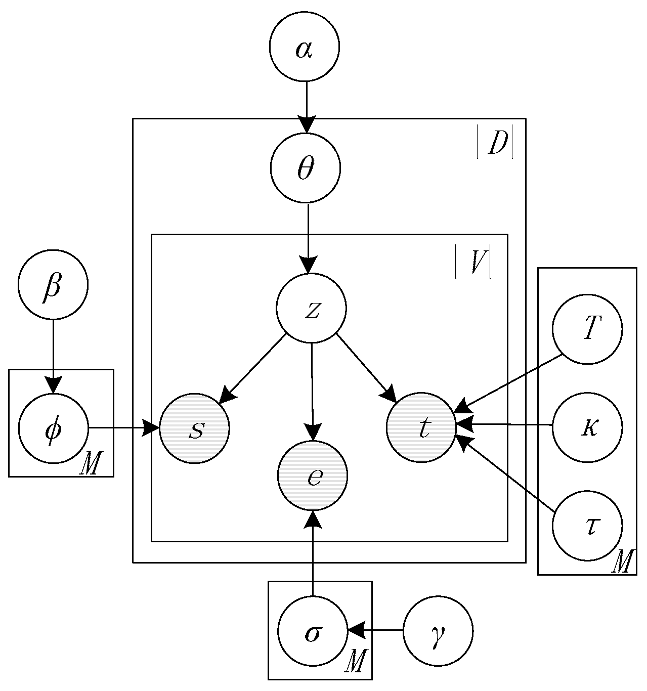
Figure 6.
Inference and modeling process of STPT.

Figure 7.
Spatial distribution of remote sensing data.

Figure 8.
Time distribution of remote sensing data.

Figure 9.
NDCGs of Top-k recommendation. (a) 7 days (time slice). (b) 14 days (time slice). (c) 30 days (time slice). (d) NDCG of STPT with different time slice.
Figure 9.
NDCGs of Top-k recommendation. (a) 7 days (time slice). (b) 14 days (time slice). (c) 30 days (time slice). (d) NDCG of STPT with different time slice.
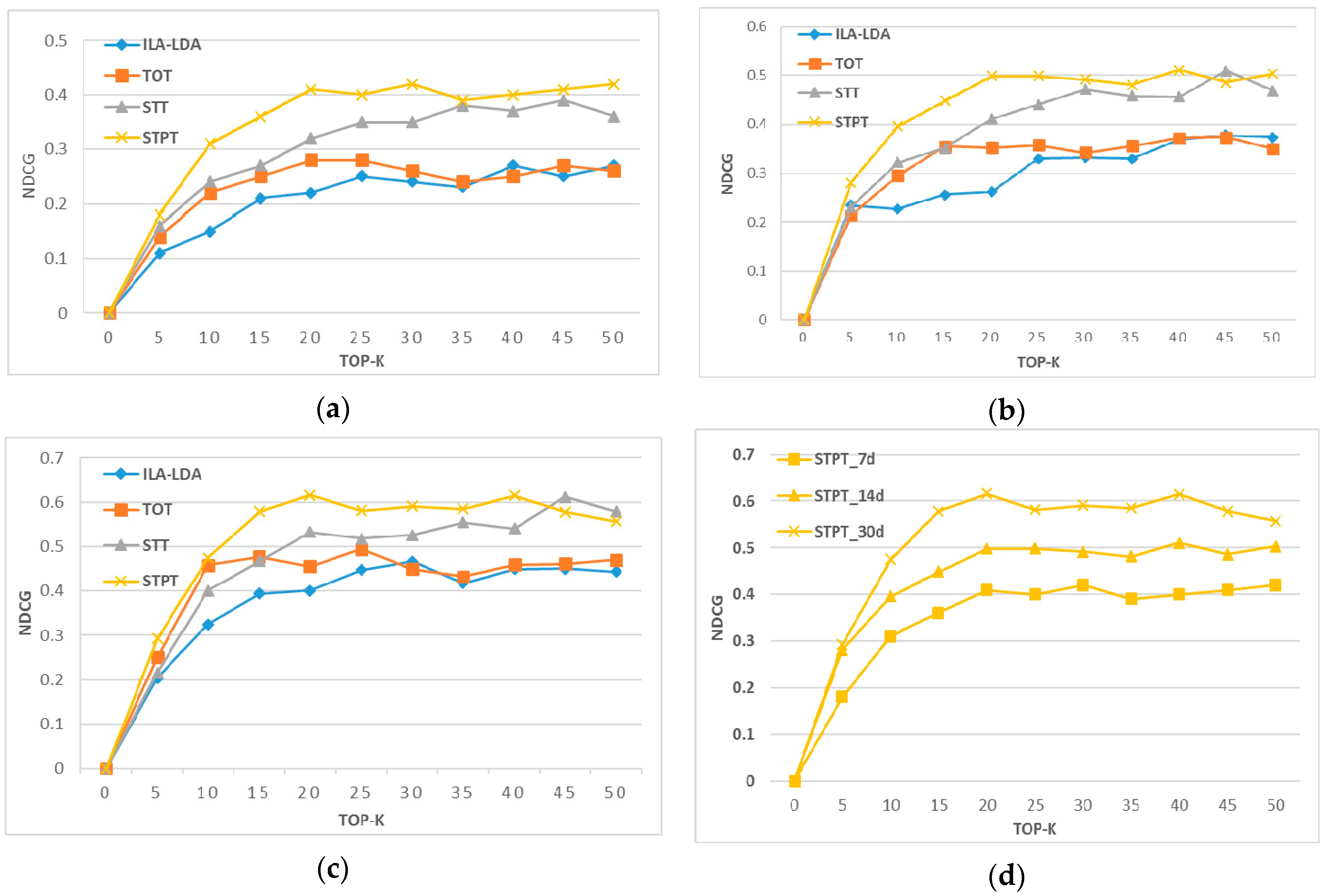
Figure 10.
The NDCG values of recommendation models for different grid sizes.
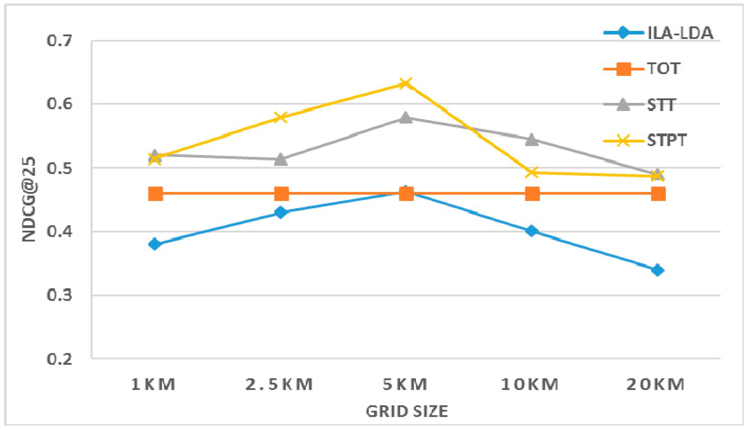
Figure 11.
The NDCG values of the recommendation models for different task numbers.
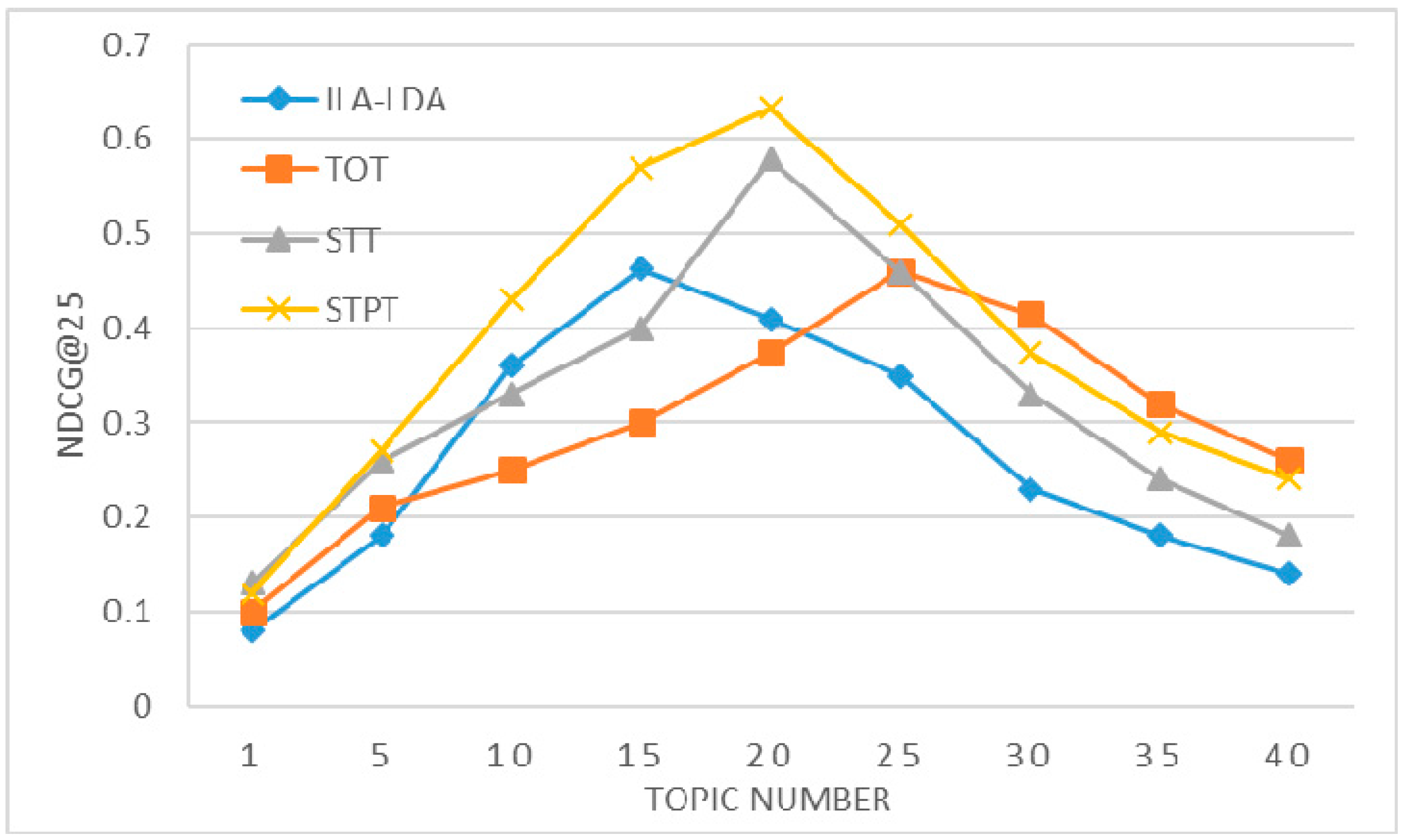
Figure 12.
Time series and their DFTs with different values of M. (a) M = 20. (b) M = 40.


Figure 13.
The probability distributions of tasks over time.
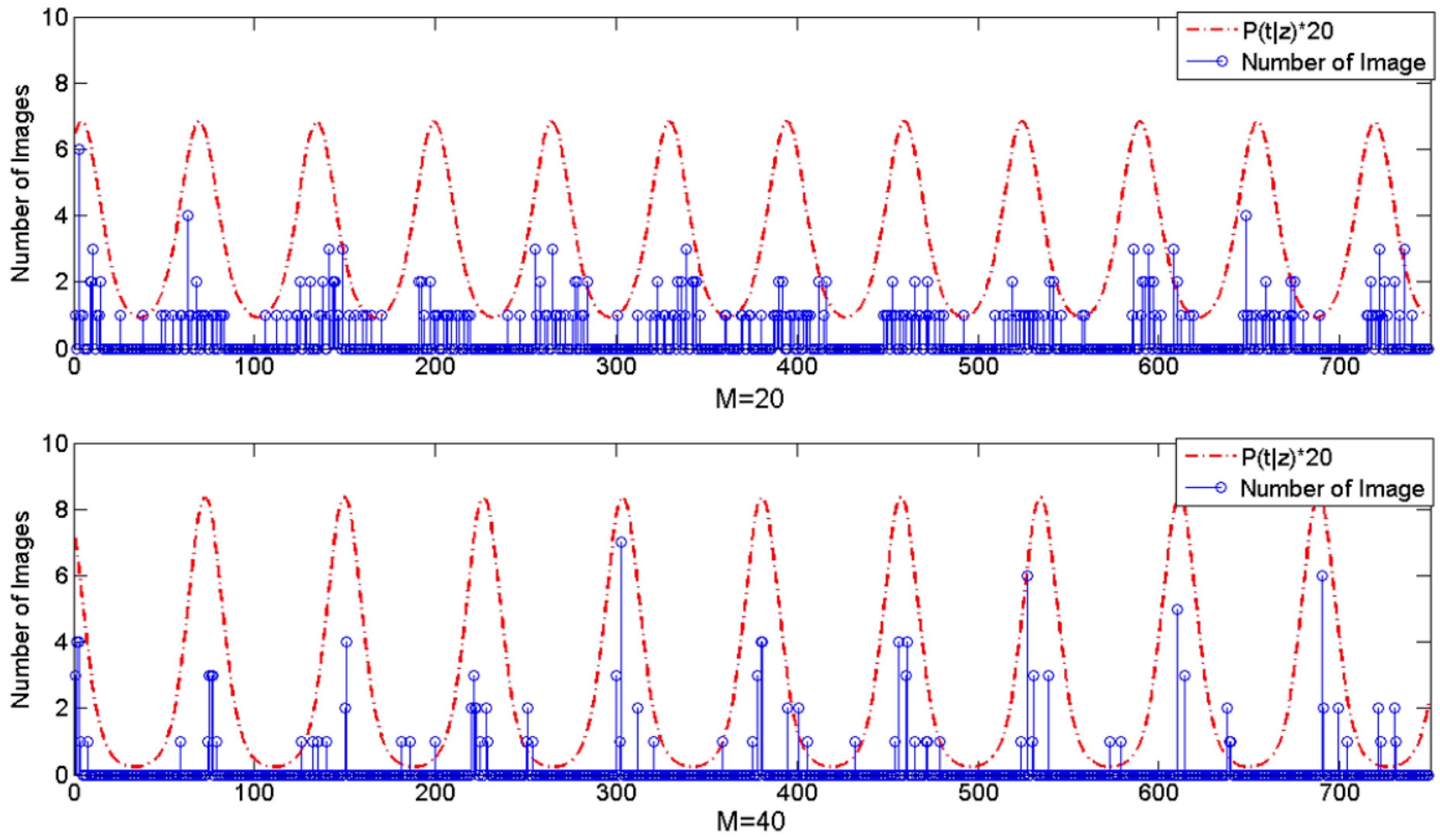
Figure 14.
Efficiency with respect to online recommendations.


Table 1.
Notations in STPT model.
| Variable | Meaning |
|---|---|
| Dr, D | a retrieval behavior document, the set of retrieval behavior documents |
| |D| | the number of retrieval behavior documents |
| S, N | the number of spatial grids and the number of image elements of RS images in the retrieval results, respectively |
| |V| | the number of RS images retrieved by each retrieval behavior |
| M | the number of tasks |
| z | latent task |
| s | the collection of spatial location grids for each RS image |
| T | the time period of task z |
| t | retrieval timestamp of remote sensing image |
| e | the sequence of image elements for each RS image |
| θ | the multinomial distributions of tasks specific to the retrieval behavior document Dr |
| ϕ | the multinomial distributions of spatial grid specific to task z: S × M matrix |
| σ | the multinomial distributions of image elements s specific to task z: N × M matrix |
| α, β, γ | the hyper parameters of the Dirichlet priors for multinomial distributions θ, ϕ, σ, respectively |
| κ | a reciprocal measure of dispersion (for the von Mises distribution) |
| τ | the initial phase point of task z (for the von Mises distribution) |
© 2018 by the authors. Licensee MDPI, Basel, Switzerland. This article is an open access article distributed under the terms and conditions of the Creative Commons Attribution (CC BY) license (http://creativecommons.org/licenses/by/4.0/).
Share and Cite
MDPI and ACS Style
Zhang, X.; Chen, D.; Liu, J. A Space-Time Periodic Task Model for Recommendation of Remote Sensing Images. ISPRS Int. J. Geo-Inf. 2018, 7, 40. https://doi.org/10.3390/ijgi7020040
AMA Style
Zhang X, Chen D, Liu J. A Space-Time Periodic Task Model for Recommendation of Remote Sensing Images. ISPRS International Journal of Geo-Information. 2018; 7(2):40. https://doi.org/10.3390/ijgi7020040
Chicago/Turabian StyleZhang, Xiuhong, Di Chen, and Jiping Liu. 2018. "A Space-Time Periodic Task Model for Recommendation of Remote Sensing Images" ISPRS International Journal of Geo-Information 7, no. 2: 40. https://doi.org/10.3390/ijgi7020040
Note that from the first issue of 2016, this journal uses article numbers instead of page numbers. See further details here.