
A Multiple Ant Colony Optimization Algorithm for Indoor Room Optimal Spatial Allocation


1
Institute of Remote Sensing and Digital Earth, Chinese Academy of Sciences, Beijing 100864, China
2
Department of Geography, University of Wisconsin-Madison, Madison, WI 53706, USA
*
Author to whom correspondence should be addressed.
ISPRS Int. J. Geo-Inf. 2017, 6(6), 161; https://doi.org/10.3390/ijgi6060161
Submission received: 4 March 2017
/
Revised: 17 May 2017
/
Accepted: 24 May 2017
/
Published: 1 June 2017
(This article belongs to the Special Issue 3D Indoor Modelling and Navigation)
Abstract
:Indoor room optimal allocation is of great importance in geographic information science (GIS) applications because it can generate effective indoor spatial patterns that improve human behavior and efficiency. However, few research concerning indoor room optimal allocation has been reported. Using an office building as an example, this paper presents an integrative approach for indoor room optimal allocation, which includes an indoor room allocation optimization model, indoor connective map design, and a multiple ant colony optimization (MACO) algorithm. The mathematical optimization model is a minimized model that integrates three types of area-weighted costs while considering the minimal requirements of each department to be allocated. The indoor connective map, which is an essential data input, is abstracted by all floor plan space partitions and connectivity between every two adjacent floors. A MACO algorithm coupled with three strategies, namely, (1) heuristic information, (2) two-colony rules, and (3) local search, is effective in achieving a feasible solution of satisfactory quality within a reasonable computation time. A case study was conducted to validate the proposed approach. The results show that the MACO algorithm with these three strategies outperforms other types of ant colony optimization (ACO), Genetic Algorithm (GA), and particle swarm optimization (PSO) algorithms in quality and stability, which demonstrates that the proposed approach is an effective technique for generating optimal indoor room spatial patterns.
1. Introduction
Humans spend almost 87% of their time indoors [1]. It is important to conduct research in indoor spaces. Some studies have already been performed, such as representation and space subdivision of indoor spaces [2,3], which provided a thorough technical foundation for further research, such as indoor room optimal allocation.
In the problem of indoor room optimal allocation, spatial search approaches are used to allocate specific objects (such as different office departments) to proper indoor space units (such as rooms) to achieve an optimal spatial layout by considering multiple factors, such as spatial convenience and personal preference. Skillful indoor spatial allocation, such as reasonably allocated departments in an office building, can effectively reduce the cost of office communication. Poor allocation can lead to increased office costs and waste. However, to the best of our knowledge, few studies have been conducted that focus on indoor room optimal allocation.
Previous studies for spatial optimal allocation involve urban planning, such as city land-use optimal allocation [4,5,6,7,8,9], protected ecological area partitioning [10], and farmland management [11]. While establishing models for these problems, macroscopic factors, such as the natural environment (such as land use suitability, compatibility), economic development (such as land use conversion cost, travel time), and spatial/geometrical characteristics (such as distance, contiguity, and compactness) usually are considered [7]. However human factors, such as the distribution of population and jobs, are always abstracted and simplified [12]. However, in an indoor environment, human factors are important because human behavior is closely coupled with the indoor spatial layout [13]. Therefore, human behavior, requirements, and their interaction with the indoor environment should be emphatically taken into consideration during problem modeling.
Moreover, similar to the spatial optimal allocation in urban planning, indoor room allocation is an non-deterministic polynomial-time hard (NP-hard) problem in the discrete domain, whose optimal solution often lies within innumerable combinations of allocable rooms and type alternatives and is hard to be found by traditional Geographic information sciences (GIS) functions within a reasonable time. Previous studies proved that the heuristic algorithm is effective at finding near-optimal solutions by obtaining a trade-off between the quality of solutions and the burden of computation. Numerous heuristic algorithms such as genetic algorithm (GA) [4,14,15,16], simulated annealing (SA) [9,17], artificial immune system (AIS) [6], particle swarm optimization (PSO) [8,18], artificial bee colony (ABC) [5,10], and ant colony optimization (ACO) [7,19] have been proposed as approaches to spatial optimal allocation in urban planning.
Among these algorithms, ACO, which simulates a set of cooperating artificial ants seeking optimal routes (solutions) by local heuristics and knowledge from past experiences [20], is special because of its unique way of constructing solutions. Many heuristic algorithms, such as GA, AIS, PSO, and ABC, construct a new solution by neighborhood search manipulation (such as crossover and mutation) that changes parts of the current solution. Although the random neighborhood search manipulation increases the solution’s diversity, it also leads to the generation of a large amount of low quality solutions because heuristic information cannot be generally used in the neighborhood search procedure, such as the commonly used crossover strategy. Different from it, ACO constructs a new solution by determining each element of a solution pseudo-randomly one by one. It means that heuristic information, which is helpful for obtaining an optimal solution of relative high quality [17], can be applied for the determination of each solution element. Potentially, ACO could be a more effective algorithm to tackle complex spatial optimization problems in certain areas.
In the area of spatial optimal allocation, ACO has been used to tackle this kind of problem. Li modified the ACO method for zoning protected natural areas by adjusting three strategies, route selection probability, heuristic information, and pheromone deposition [19]. However, the proposed ACO can only be used to handle the land use allocation problem that involves only one land use type. Liu used a multi-type ant colony optimization (ACO) method to solve the problem with multiple land use types in large areas [7]. In his modified ACO algorithms, the types of ants correspond to the types of land uses; the ant colony size equals the number of allocable units in study region, and each ant occupies a unit according to site selection probabilities. The locations of all the ants form a solution of the land use allocation problem. It can be seen that the colony size is not scalable and only one solution is obtained in each iteration, which is different from the essence of ACO that positively feeds back by the current-best solution among multiple solutions obtained by multiple ants in each iteration. Moreover, because only one solution is found in each iteration, it will reduce the solution’s diversity, and will thus be trapped into the local optimal solution easily. Therefore, it is not suitable to introduce the modified ACO to solve the indoor room allocation problem directly.
Based on the above analysis, this paper presents an optimal model considering human interaction for indoor spatial allocation. A new multiple ant colony optimization (MACO) algorithm that is able to effectively allocate multiple objects to indoor space units is proposed to solve this NP-hard problem. The remainder of the paper is arranged as follows. Section 2 and Section 3 introduce the details of the approach, including indoor spatial data organization, optimization model construction, and MACO resolution. The approach is tested and illustrated with a case study in Section 4. Finally, Section 5 presents the discussion and conclusions drawn based on previous experiments.
2. Model Formulation
2.1. Indoor Room Optimal Allocation Model
The goal of establishing an indoor room optimal allocation model is to make the connectivity cost of people’s communication minimized, the spatial layout of relative departments concentrated, and the energy consumption reduced. Different optimal allocation models could be established according to different requirements. For example, in this paper, the following demands are considered. (1) To ensure the efficiency of internal communication, the rooms that are assigned to the same office department number should be relatively compact; (2) To enhance the convenience of daily work, the total connectivity cost of the business department’s rooms to the public department’s rooms should be minimized; (3) To reduce the energy consumption by utilizing elevators, the total connectivity cost of all allocated rooms to the building’s exits is low; (4) Considering sustainable development, ensuring convenience and satisfying all department demands, the remaining rooms’ area should be as large as possible.
In this paper, the mathematic symbols used in the model establishment are listed in Table 1.
Based on the first three requirements, three kinds of connectivity cost are defined, (1) (shown in Formula (1)), the connectivity cost within the same department, (2) (shown in Formula (2) ), the connectivity cost of all business departments’ rooms to public departments’, and (3) (shown in Formula (3)), the total connectivity cost from all allocated rooms to the building’s exits. Meanwhile, considering the fourth requirement, all three connectivity costs are weighted by the room area.
Therefore, we can allocate departments with the minimum value for the following functions.
Formula (5) is the area constraint, which requires that the total area of allocated rooms for each department must be larger than the department’s minimum area demand.
The computation scale of the problem is , which will increase dramatically with the increase of , and . It is extremely difficult to find the best solution by greedy searches. Therefore, it is necessary to use a proper heuristic algorithm to find the optimal solution within reasonable time.
2.2. Indoor Spatial Data Model
The goal of designing indoor spatial data is to obtain the required parameters while solving the optimization problem, such as the connectivity cost between every two rooms , and each room’s area .
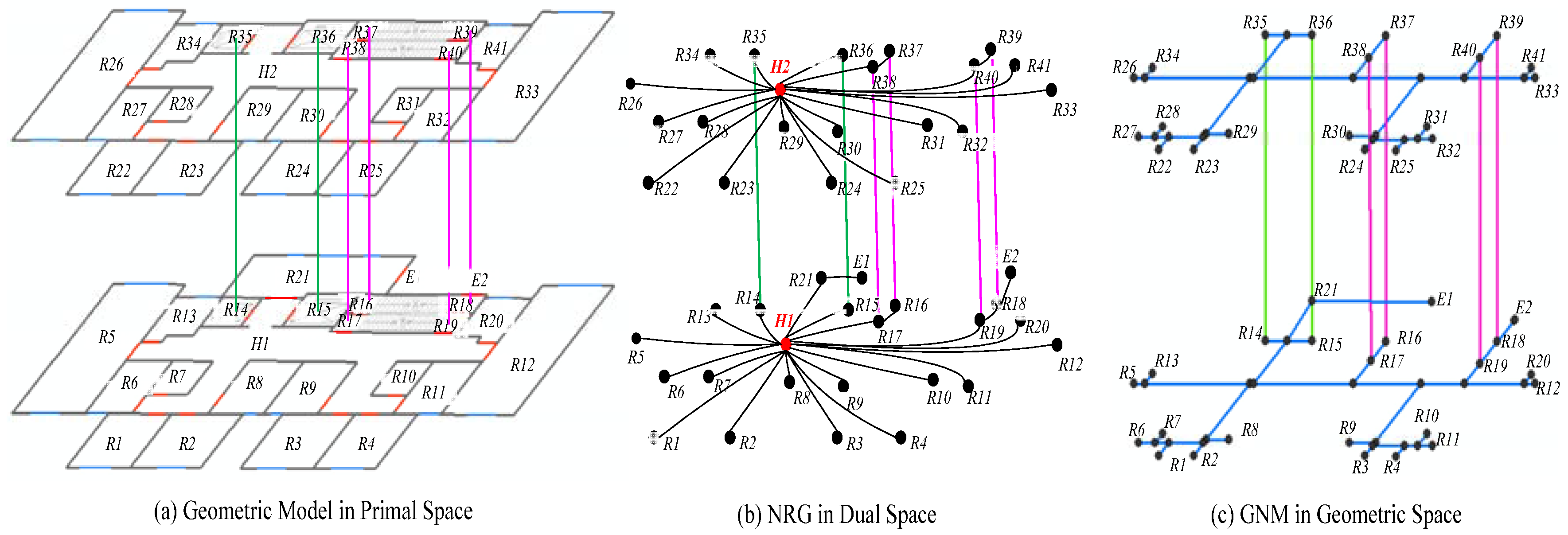
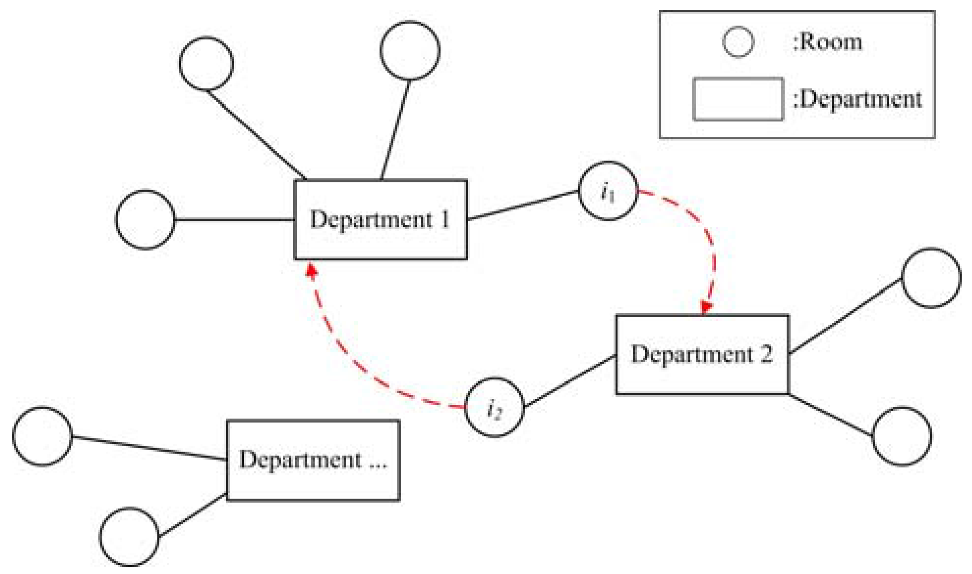
In order to be supportive for obtaining the connectivity cost , the Geometric Network Model (GNM) [21] is imported to model the indoor spatial data. GNM is derived from a logical network, such as the Node-Relation Graph (NRG) in OGC IndoorGML [22], and is used to geometrically and realistically represent the indoor connectivity relationships. Similar to NRG, GNM represents 3D entities (such as rooms, exits, corridors) as nodes in a graph in dual space [23]. However, different from the abstraction of a simple polygon (such as a hallway) to a node in NRG, GNM defines it as line segments. As shown in Figure 1, Figure 1b is the abstraction of an indoor building in primal space (Figure 1a) by the NRG models, but its two hallway nodes (H1 and H2) are represented as line features in the GNM models (shown as the blue line segments in Figure 1c).
In this paper, the main partitions in each floor plan, such as each room, exits, lift lobbies, and staircases, are abstracted as nodes located in each partition’s entrance. In each floor plan and between floors, connections (such as hallways, stairs, and elevators) are abstracted as edges to represent the connectivity among different partitions. Notably, the area of each room and the connectivity costs of each connection should be geographically calculated in primal geographic space.
Based on the indoor connectivity data, an origins and destinations (OD) cost matrix is obtained by setting the point features of all allocable rooms and building exits as origins and destinations. This matrix and each allocable room’s area are used in the optimization computation as inputs.
3. Multiple Ant Colony Optimization
3.1. Basic ACO
ACO is a type of swarm intelligence heuristic algorithm that simulates the behaviors and communication of ants to solve complex optimization problems [20]. In general, five phases are included in a basic ACO algorithm.
(1) Initializing pheromones. Usually, the pheromone on each node is initialized as the same value.
(2) Constructing solutions. Each artificial ant selects route nodes (solution’s elements) successively and pseudo-randomly according to the transition probability to form a route (a solution). The transition probability is determined by the pheromones on all nodes and the heuristic information. Commonly, the more pheromone deposited on a node, the higher the probability that the node is selected by an ant.
(3) Updating solutions. If a better solution is constructed, the best-so-far solution will be recorded as the better one.
(4) Updating the pheromones on all nodes after new solutions are constructed by ants. This contains two kinds of pheromone updating strategies. One is pheromone reinforcement, which is used to increase the pheromone on each solution’s nodes. The better the solution is, the larger the pheromone increment is. The other one is pheromone evaporation, which makes the pheromone on all nodes decrease at a predefined rate and is helpful for ants to “forget” the bad solutions in the previous iteration. By the combination of these two strategies and multiple repeated iterations, the pheromones on the optimal route’s nodes increase, thus, the ants tend to converge to the optimal path (the optimal solution).
(5) Judging the algorithm’s convergence. The convergent condition is usually defined as a maximum iteration number or maximum iteration time. If the convergent condition is not met, step 2 and step 3 will be executed again, otherwise, the algorithm stops.
3.2. Improvement Strategies
Based on the basic ACO algorithm, this paper proposes multiple ant colony optimization (MACO) to solve the problem of indoor spatial optimal allocation. Compared to basic ACO, MACO is improved from three aspects. First, three kinds of heuristic information that are influential to the transition probability calculation are proposed to navigate each ant’s route selection to areas in the solution space where the global optimal solution is located. Second, a two-colony optimization rule is proposed to prevent the ants’ route selection from being trapped in the local optimal solution. Third, a local search strategy is imported to improve the best solution’s quality in each iteration and also the algorithm’s overall performance.
3.2.1. Heuristic Information
When implementing indoor spatial allocation, if a fully random strategy is adopted, a large number of solutions with low quality will be generated, which makes it challenging to find the optimal solution within a reasonable time. Therefore, in this MACO, three types of connectivity costs in the problem’s optimization model (the minimum connectivity cost of allocated rooms and exits, the minimum connectivity cost among rooms that are assigned to the same department, and the minimum connectivity costs between rooms that belong to different departments) can be treated as the heuristic information for assigning rooms to each department.
While evaluating the heuristic information, the mathematic symbols are listed as follows (Table 2).
Explicitly, heuristic information can be calculated based on the following three circumstances.
- If or if and , then , which is the reciprocal of the minimum weighted connectivity cost between the allocated room and the building exits.
- If and , then , which is the reciprocal of the minimum weighted connectivity cost between the allocated room and the allocated rooms whose department type is not .
- If , then , which is the reciprocal of the minimum weighted connectivity cost between the allocated room and the allocated rooms whose department number is .
3.2.2. Two-Colony Optimization Strategy
Because of the usage of these three types of heuristic information, the order of allocating departments has a strong impact on the final allocation solution. In order to ensure more opportunities for generating solutions with a better order of allocating departments, a two-colony optimization rule has been imported to MACO. These two ant colonies are of the same size, .
In the phase of solution generation, the first ant colony is used to pseudo-randomly determine the optimal order of allocating departments according to the transition probability based on the pheromone. The first-colony pheromone matrix is , in which is the number of the department and is the allocation order. If the allocation order of department is and the former departments’ allocating order set is , the transition probability that the allocating order of department is set as is:
in which is the adjustment parameter of pheromone .
Based on the order obtained by the first colony, the second ant colony assigns rooms to each department to form solutions (a sample of the solution is shown in Figure 2) according to its transition probability. The probability is highly related to the heuristic information mentioned in Section 3.2.1 and the second-colony’s pheromones. The second-colony pheromone matrix is , in which is the number of departments and is the number of rooms. The transition probability that a room is assigned to department can be expressed as Formula (8):
in which , are the adjustment parameters of pheromone and heuristic information respectively. The meanings of and can be found in Table 2.
In the phase of pheromone updating, the two colonies use the same elite ant strategy via two pheromone matrixes, and (Formulas (9)–(11)):
Here, the pheromone and of node in and during the iteration are represented by the same symbol . is the pheromone decay parameter, is the pheromone increment on all nodes of the current best solution in iteration , is the pheromone increment of the best-so-far solution , is the best objective function value in iteration , and is the best function value of the best-so-far solution. is a predefined constant, which is used to ensure that the pheromone increments, and , are not too large to lead to a local optimal solution or too small to result in slow convergence relative to the pheromone and .
3.2.3. Local Search
In this MACO, if all ants finish constructing solutions, a greedy local search strategy, swap exchange, is used to further improve the solution quality. This strategy swaps two rooms that were originally assigned to different departments to generate a new solution (shown in Figure 3). Because a local search is a time consuming operation, it is only applied to the best solution in the current iteration .
The procedure of the local search can be expressed as follows.
- Calculate the accumulated connectivity cost between each room that is assigned to department and the other rooms.
- Select the number of rooms and all unallocated rooms to form an allocable room set .
- Randomly swap two rooms , and calculate the new solution’s objective function value. Find the swap operation with the largest improvement value, execute this swap to obtain a new solution , and let .
3.3. Overall Procedure
The overall procedure can be explicitly described as follows.
Input: (1) Indoor connective map, which includes allocable rooms, building exits, room areas, and connectivity costs; (2) allocation demand data, such as department types and each department’s spatial area requirements; and (3) ACO parameters, such as population size , adjustment parameters of the pheromone and heuristic information , pheromone update constant and decay parameter , and the maximum iteration number .
Step 1: Initialize the data, such as the pheromone matrix and and the iteration number .
Step 2: Execute Steps 2.1–2.3 by each ant to construct solutions.
Step 2.0: Set ant counter .
Step 2.1: The ant in the first ant colony determines the departments’ allocating order. Execute steps 2.1.1–2.1.5.
Step 2.1.1: Set departments’ counter , departments’ allocating order .
Step 2.1.2: If , go to step 2.1.3, otherwise, go to step 2.2.
Step 2.1.3: Calculate the transition probability by Formula (7) according to pheromone matrix .
Step 2.1.3: Calculate the distribution of transition probabilities, .
Step 2.1.4: Generate a random number , select the value () as the allocating order of department , .
Step 2.1.5: , . Go to step 2.1.2.
Step 2.2: Based on the order obtained in Step 2.1, the ant in the second colony assign rooms to each department to obtain a solution. Execute steps 2.2.1–2.2.10.
Step 2.2.1: Set departments’ counter , the allocable rooms set , and the allocation solution as a zero matrix .
Step 2.2.2: If , go to step 2.2.3, otherwise, go to step 2.3.
Step 2.2.3: Determine the department that will be allocated in the current calculation, .
Step 2.2.4: Calculate the heuristic information according to Section 3.2.1.
Step 2.2.5: Calculate the transition probability by Formula (8) according to the pheromone matrix and the heuristic information obtained in step 2.2.4.
Step 2.2.6: Calculate the distribution of transition probabilities, .
Step 2.2.7: Generate a random number , and select the value () as the room that was allocated to department , .
Step 2.2.8: Update the set of allocable rooms, .
Step 2.2.9: If , go to step 2.2.10, otherwise, go to step 2.2.4.
Step 2.2.10: . Go to step 2.2.2.
Step 2.3: Update the current-best solution.
Step 2.3.1: Calculate the objective function value according to Formulas (1)–(4).
Step 2.3.2: If , go to step 2.3.3, otherwise, go to step 2.4.
Step 2.3.3: Update the current-best objective function value , the current best allocating order of departments , and the current-best room allocation solution .
Step 2.4: , if , go to step 2.1, otherwise, go to step 3.
Step 3: Apply local search to the best solution in the current iteration to further improve the quality of the current-best solution.
Step 4: Update the best-so-far solution.
Step 4.1: If , go to step 4,2, otherwise, go to step 5.
Step 4.2: Update the best-so-far objective function value , the best-so-far allocating order of departments , and the best-so-far room allocation solution .
Step 5: Update the pheromone Matrix and by Formulas (9)–(11).
Step 6: Set g = g + 1. Evaluate the convergence. If , repeat steps 2–5; otherwise, stop.
Output: The best-so-far solution .
3.4. Time Complexity
In this paper, the quantities of departments and rooms are and , respectively, the maximum iteration number is , and the size of ant colony is . The MACO algorithm’s computational time complexity can be analyzed as follows.
4. Experiment
In this experiment, the proposed MACO algorithm is coded in MATLAB 2012b software and implemented on a PC with an Intel (R) Xeon (R) CPU E3-1230 @ 3.3 GHz and 16 GB RAM using the Windows 7 64-bit operating system.
4.1. Experimental Data Description
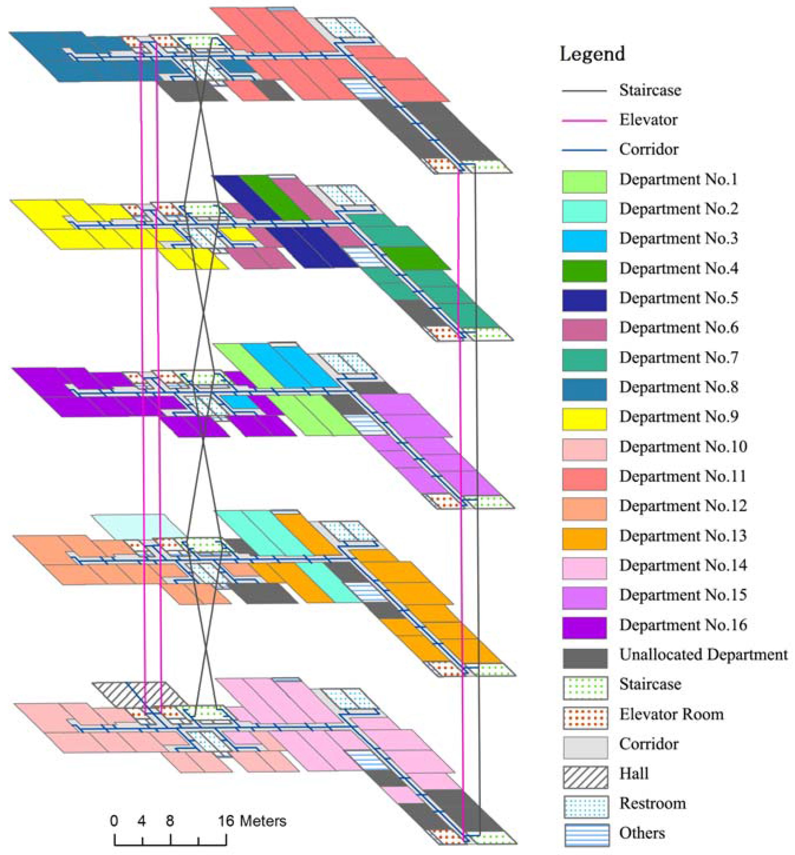
This paper uses an office building as a case study. The building contains five floors, three elevators, and three staircases. There are 145 allocable rooms of different areas. The total area is 3089 m2, the smallest area is 8 m2, and the largest area is 36 m2. Considering factors such as electric energy savings and strenuous stair climbing, the connectivity cost of each elevator that connects two adjacent floors is 10 meters, and each staircase’s connectivity cost is 12 m. The connectivity cost of rooms on the same floor is set as its practical connective distance.
4.2. MACO Parameter Selection
The main parameters concerning MACO include , , , , , , and . In this experiment, the converging condition is set as , or the current-best solution is the best-so-far solution for ten successive times. Based on the preliminary experiment and experiences [19,24,25], an orthogonal experimental approach was used to determine the values of these parameters among the following value ranges: , , , , , and . The parameter selection experiments were designed as shown in Table 6. Each experiment was run ten times.
Based on the range analysis method of orthogonal experiments [26], the results are summarized in Table 7. is the average value of all solutions’ objective function value, while the corresponding parameter value is set as the value in its candidate value range. For example, the number 25.39355 in the first row and first column refers to the average objective value of all solutions with . The range is the gap between the maximum and minimum value, which reflects the objective’s fluctuation range with the change of a single parameter’s value. A larger value of implies a more important influence of the corresponding parameter on the final results. Therefore, the primary order of the six parameters is . The optimal parameters’ value is the value in its candidate range if maintains the minimum objective value. Therefore, the suggested parameter values are , , , , , and .
4.3. Experimental Results and Analysis
Based on the parameter selection experiments, we obtain a set of parameters , , , , , and , that are expected to achieve favorable results.
One optimal MACO solution was selected for result analysis, and its statistic result is summarized in Table 8. Because of the area-weighted connectivity cost in the optimization model, it is impossible for an optimal solution to assign too many rooms to a department. From the table, we find that the area of each department’s allocated rooms is close to its required minimal area. This result is reasonable for meeting the sustainable development requirement; the remaining rooms’ area should be as large as possible, while ensuring convenience and satisfying all department demands.
The solution’s spatial allocation is depicted in Figure 5. From the figure, it can be found that almost all of the public departments are centered on the middle floors to reduce the connectivity cost to other business departments, which matches our common experience. Besides, we find that the rooms assigned to the same department are concentrated on the same floor; this condition arises because of the sufficient allocable rooms in each floor and relatively large connectivity cost settings of elevators and staircases between two adjacent floors while considering factors such as electric energy saving and stair climbing. As a result, the unallocated rooms on one floor are not assigned to a department if their areas cannot satisfy any department’s minimal requirements. Thus, it is reasonable that some rooms are unallocated on low floors, even though they may increase the connectivity cost of all allocated rooms to building exits.
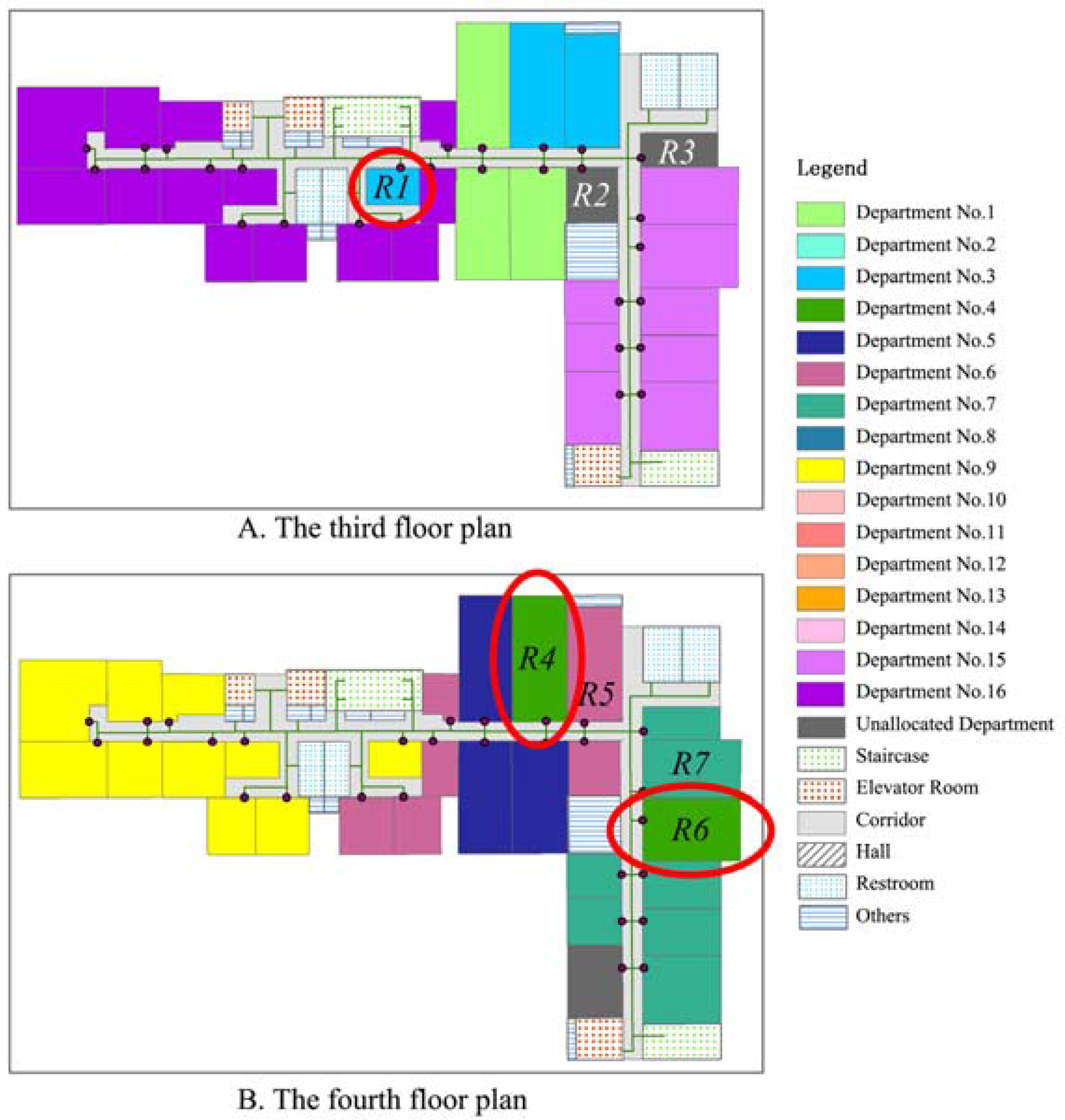
Notably, a few department rooms are not closely concentrated, shown as the rooms in red ovals in Figure 6. In Figure 6A, the rooms of department 3, in the red circle, are not effectively spatially close to other rooms with the same department number, because all the connectivity costs are weighted by room areas. The area of all rooms labeled as department 3 is 80 m2, equal to the department’s minimal area demand. If room (16 m2) or room (14 m2) but not room (11 m2) are assigned to department 3, the area-weighted connectivity costs would increase and result in a worse objective function value, which was approved by executing local search operations. Similar to the situation that occurred in the third floor (Figure 6B), rooms and with the same department number are separated. From the perspective of spatial aggregation, if the types of rooms and were exchanged, or the types of rooms and were exchanged, the costs within the same department, , would be reduced. However, the exchange trials show that the cost between business and public departments, , will increase at a greater rate, which can be seen in Table 9. It proves the optimality and reasonability of the solution generated by MACO.
4.4. Algorithm Validation
4.4.1. Comparison of the Improved Strategies
The proposed MACO algorithm is compared with three other types of ACO methods with different strategies (shown in Table 10). ACO-1 does not use the heuristic information while calculating the transition probability to form a solution. Compared to MACO’s overall procedure, ACO-1 will not execute step 2.2.4, and the probability’s calculation in step 2.2.5 is based on Formula (7) rather than Formula (8). ACO-2 does not use the local search strategy to further improve the current-best solution’s quality, whose procedure is the same as MACO’s procedure without step 3. ACO-3 utilizes only one ant colony to construct a solution. Instead of the first ant colony determining the order of allocating departments pseudo-randomly in MACO, the order of allocating departments is totally determined randomly in ACO-3. It means that its overall procedure does not contain all the operations on the first colony in MACO, which mainly include step 2.1 and step 5 concerning the updating pheromone matrix .
The statistical results of the experiments after ten iterations of each algorithm are shown in Table 11.
Table 11 clearly shows that MACO using the strategies proposed in this paper outperforms other types of ACO algorithms in quality and stability. The importance of each strategy can be observed. (1) The experiment of ACO-1 that lacks heuristic information produced the worst results, which indicates that heuristic information plays the most important role in achieving a solution of high quality. (2) The strategy of local search also plays an essential role for satisfactory results since ACO-2 that lacks local search can only obtain results ranking as second best. (3) Relative to the two strategies discussed above, the strategy of a two-colony rule plays a relatively small role in solution quality because ACO-3’s results are nearest to the MACO results. However, ACO-3 exhibited the least stability with the largest standard deviation.
The approximate computation time of these three strategies, heuristic information, local search, and two-colony rules was 0.7963, 0.2436, and 0.1849 s per iteration, respectively. These values are shown in Figure 7 with the objective function value gap from MACO without using one of these strategies. Figure 7 shows that the heuristic information strategy is relatively time consuming, but it is the most effective strategy to improve the solution quality. The total computation time of MACO is acceptable for practical application.
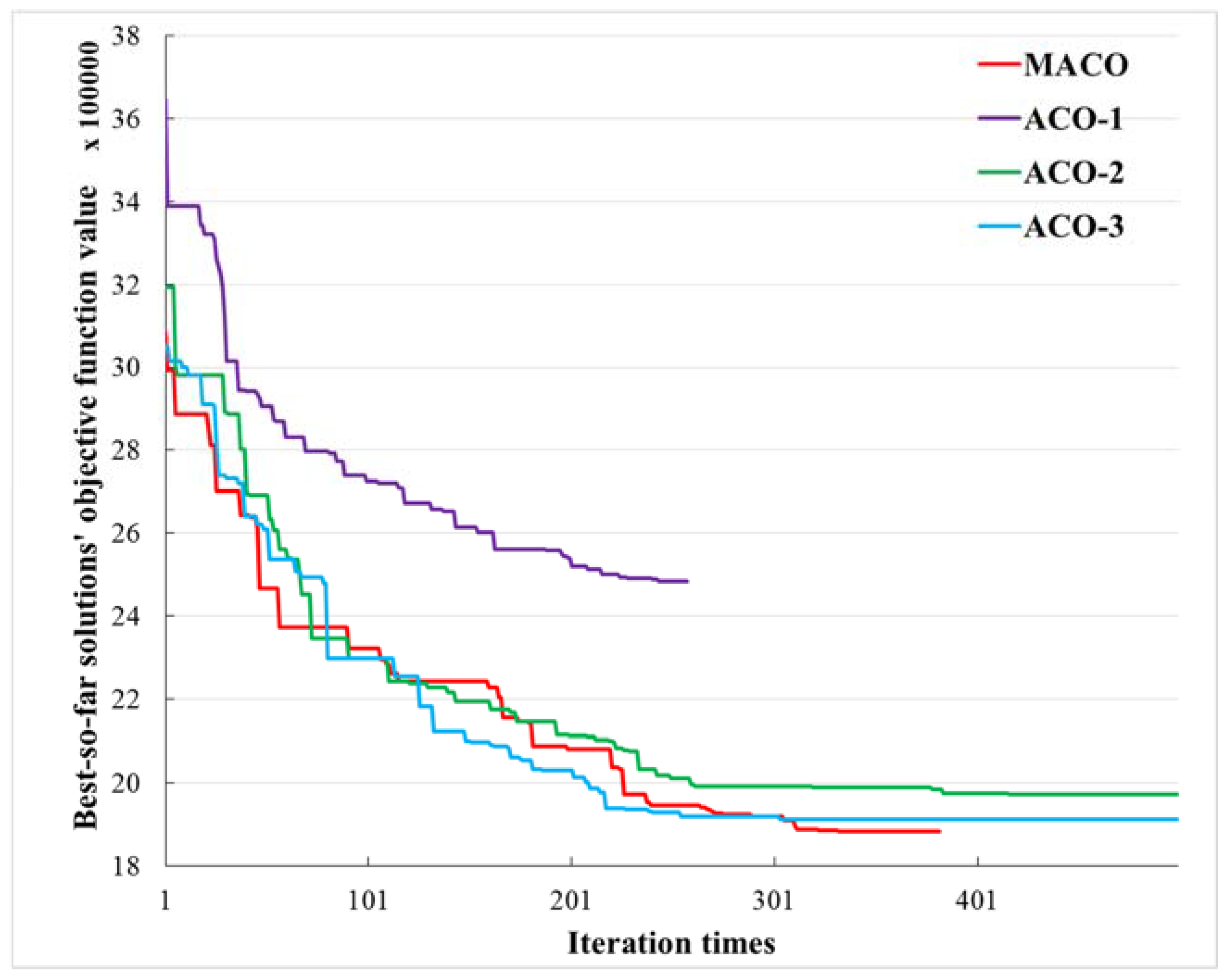
Taking each experiment’s best result as an example, the best-so-far solution found in each iteration of each algorithm is depicted in Figure 8.
The curve of ACO-1 shows that this algorithm always has the worst solution with the largest objective function value during the optimization procedure, which implies that it cannot achieve a satisfactory result without the incorporation of the heuristic information. The curves of MACO, ACO-2, and ACO-3 indicate that the objective function values are evidently optimized before the 200th iteration and that these three algorithms have similar performance while exploring new solutions. However, with the implementation of optimization, if the iteration is more than 300, MACO can achieve better solutions than ACO-2 and ACO-3. Different from ACO-2 and ACO-3, both MACO and ACO-1 provide convergence because the optimal solution is found ten successive times within 500 iterations, which means that the strategies of heuristic information and two-colony rules can effectively reduce a solution’s randomness while ensuring its diversity.
4.4.2. Comparison of the Different Algorithms
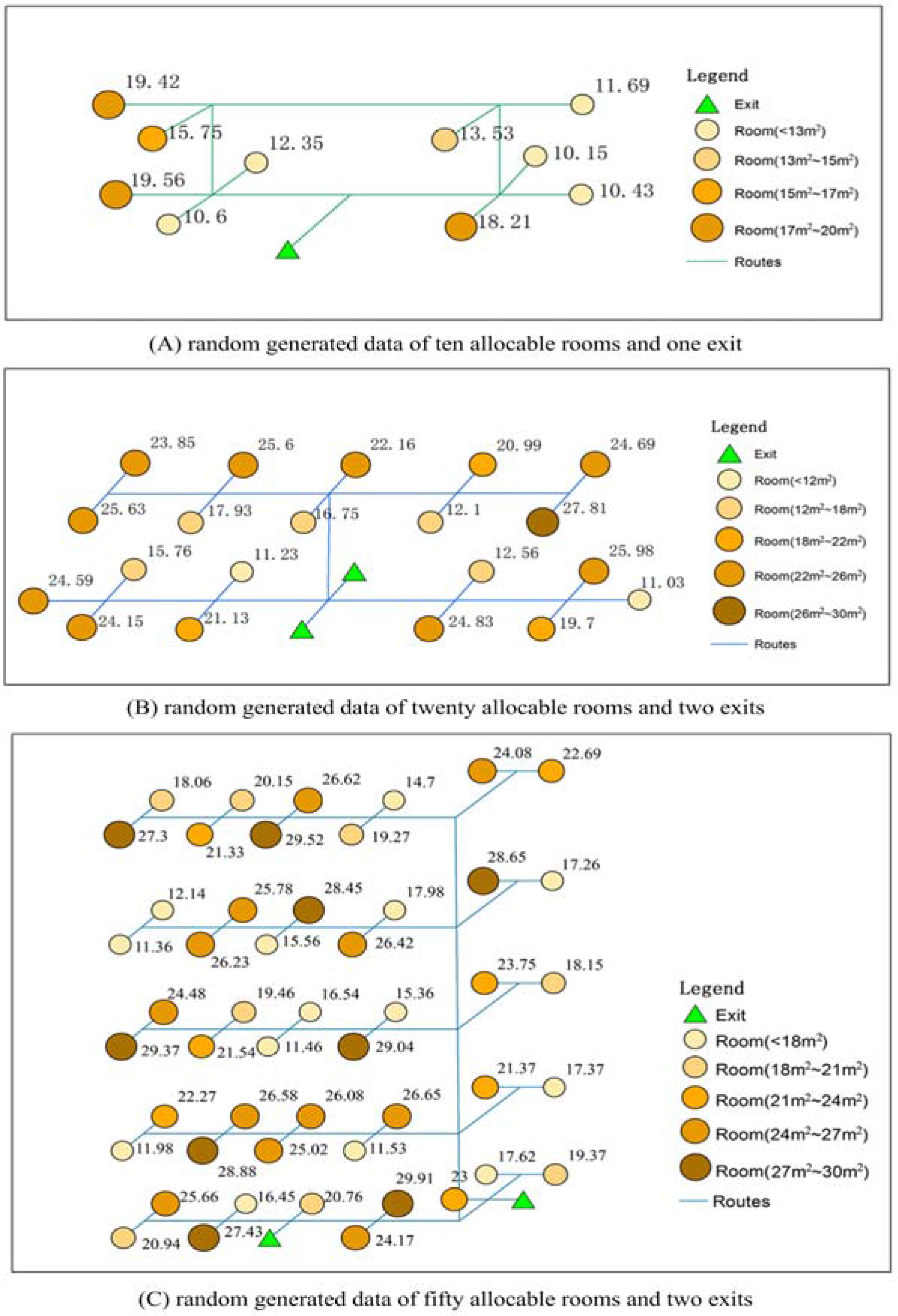
In order to validate the algorithm’s generality and effectiveness, we use three sets of simulated data and two different intelligent algorithms, Genetic Algorithm (GA) and Particle Swarm Optimization (PSO), to make comparisons. The simulated data include randomly generated indoor spatial data (shown in Figure 9) and allocation requirements (Table 12).
While using GA and PSO to solve the problem of indoor room allocation, the same strategy as MACO is used to generate the initial solutions. In the GA algorithm, crossover operations that exchange the department types of two randomly selected rooms with the same position in two solutions, and mutation operations that swap the department types of two randomly selected rooms with different positions in a solution, are combined together to generate new solutions. Similar to [8], the PSO in this comparison experiment adopts a solution neighborhood search rule with the same genetic reproduction mechanisms as GA, namely crossover and mutation, to generate new solutions. It is notable that non-feasible solutions will be easily generated by such neighborhood search strategies. Therefore, the following two steps will be adopted to adjust the non-feasible solution to being feasible.
Step 1. For each department whose allocated room area is larger than its minimal requirement , randomly select a room with the department type k and set its status as unallocated until .
Step 2. For each department k (), pseudo-randomly assign a room to it according to the probabilities determined by heuristic information mentioned in Section 3.2.1 until the department’s area demand is satisfied.
After thirty calculations with the convergent condition that the current-best solution is the best-so-far solution for ten successive times, the statistical results are listed in Table 13. It clearly shows that MACO outperforms GA and PSO in the problem of indoor room allocation with smaller objective function values and standard deviations.
5. Discussion and Conclusions
Similar to city land use allocation, indoor spatial optimal allocation is a complex process in which the complexity of searching for an optimum solution increases enormously with increases in the number of objects to be allocated and the size of the data set. However, indoor spatial optimal allocation has its own distinguishing characteristics. One is that human behavior should be considered in optimization modeling. The other is that the solving algorithm for this discrete domain problem is different since the constraints of the optimization model are more complex. Therefore, this paper derives an indoor spatial allocation model by minimizing certain area-weighted connectivity costs and proposes a MACO algorithm to solve the problem. The proposed algorithm contains three effective strategies, heuristic information, two-colony rules, and local search. A series of experiments proves that MACO is an efficient technique for generating alternative indoor allocation patterns.
This paper focused primarily on the application of an office building’s indoor spatial optimal allocation. Based on the model proposed in this paper, the objective function and constraints could be added or modified for different allocation demands in other application scenarios. The solution is easily extended to other indoor spatial allocation problems, such as allocation in school buildings and commercial centers. The indoor map processing and model optimization algorithm proposed in this paper is versatile and can accommodate other indoor spatial allocation problems.
However, some potential limitations exist that can be summarized from two points of view. First, the proposed model of indoor spatial optimal allocation is a simple version of a practical problem. For example, (1) only two types of departments, business and public, are considered in this model, (2) the tightness differences between different business departments and public departments are not considered, and (3) the demand differences of different departments for floors are not considered. Based on certain supportive data, these limitations could be eliminated. For the first limitation, the parameters of department type could be extended. For the second, the connectivity costs between business and public departments could have different weights. The higher the weight is, the closer the two departments are. For the third limitation, an index of demand suitability could be proposed, and an objective function that maximizes the total suitability could be established.
Second, ACO is a type of random algorithm, which means that it does not necessarily find the best solution; it can only provide a set of optimal solutions for the decision maker. In addition, as the scale of the data rises, the computation time of ACO increases dramatically. Methods to improve its calculation efficiency are a recommended topic for further study.
Acknowledgments
This study was supported by the National Science-technology Support Plan of China (2015BAJ02B00), the Director Foundation of Institute of Remote Sensing and Digital Earth, Chinese Academy of Sciences (Y6SJ2300CX), and the Open Research Fund of Key Laboratory of Digital Earth Science, Institute of Remote Sensing and Digital Earth, Chinese Academy of Sciences (2015LDE0020).
Author Contributions
Lina Yang. Xu Sun, and Tianhe Chi proposed the original idea of this paper; Axing Zhu improved the idea of the paper; Lina Yang conceived and designed the experiments; Xu Sun performed the experiments and analyzed the data; Lina Yang wrote the paper.
Conflicts of Interest
The authors declare no conflict of interests.
References
- Klepeis, N.E.; Nelson, W.C.; Ott, W.R.; Robinson, J.P.; Tsang, A.M.; Switzer, P.; Behar, J.V.; Hern, S.C.; Engelmann, W.H. The National Human Activity Pattern Survey (NHAPS): A resource for assessing exposure to environmental pollutants. J. Expo. Anal. Environ. Epidemiol. 2001, 11, 231–252. [Google Scholar] [CrossRef] [PubMed]
- Teo, T.; Cho, K. BIM-oriented indoor network model for indoor and outdoor combined route planning. Adv. Eng. Inform. 2016, 30, 268–282. [Google Scholar] [CrossRef]
- Jensen, C.S.; Lu, H.; Yang, B. Graph model based indoor tracking. In Proceedings of the Mobile Data Management: Systems, Services and Middleware, Taipei, Taiwan, 18–20 May 2009; pp. 122–131. [Google Scholar]
- Huang, B.; Zhang, W. Sustainable Land-Use planning for a downtown lake area in central China: Multiobjective optimization approach aided by urban growth modeling. J. Urban Plan. Dev. 2014, 140, 1–12. [Google Scholar] [CrossRef]
- Yang, L.; Sun, X.; Peng, L.; Shao, J.; Chi, T. An improved artificial bee colony algorithm for optimal land-use allocation. Int. J. Geogr. Inf. Sci. 2015, 29, 1470–1489. [Google Scholar] [CrossRef]
- Huang, K.; Liu, X.; Li, X.; Liang, J.; He, S. An improved artificial immune system for seeking the Pareto front of land-use allocation problem in large areas. Int. J. Geogr. Inf. Sci. 2013, 27, 922–946. [Google Scholar] [CrossRef]
- Liu, X.; Li, X.; Shi, X.; Huang, K.; Liu, Y. A multi-type ant colony optimization (MACO) method for optimal land use allocation in large areas. Int. J. Geogr. Inf. Sci. 2012, 26, 1325–1343. [Google Scholar] [CrossRef]
- Liu, X.; Ou, J.; Li, X.; Ai, B. Combining system dynamics and hybrid particle swarm optimization for land use allocation. Ecol. Model. 2013, 257, 11–24. [Google Scholar] [CrossRef]
- Sante-Riveira, I.; Boullon-Magan, M.; Crecente-Maseda, R.; Miranda-Barros, D. Algorithm based on simulated annealing for land-use allocation. Comput. Geosci. UK 2008, 34, 259–268. [Google Scholar] [CrossRef]
- Shao, J.; Yang, L.; Peng, L.; Chi, T.; Wang, X. An improved artificial bee Colony-Based approach for zoning protected ecological areas. PLoS ONE 2015, 10, e0137880. [Google Scholar] [CrossRef] [PubMed]
- Liu, X.; Li, X.; Tan, Z.; Chen, Y. Zoning farmland protection under spatial constraints by integrating remote sensing, GIS and artificial immune systems. Int. J. Geogr. Inf. Sci. 2011, 25, 1829–1848. [Google Scholar] [CrossRef]
- Vanegas, C.A.; Aliaga, D.G.; Benes, B.; Waddell, P.A. Interactive Design of Urban Spaces Using Geometrical and Behavioral Modeling; ACM: New York, NY, USA, 2009. [Google Scholar]
- Feng, T.; Yu, L.; Yeung, S.; Yin, K.; Zhou, K. Crowd-driven mid-scale layout design. ACM Trans. Graph. 2016, 35, 1–14. [Google Scholar] [CrossRef]
- Li, X.; Yeh, A. Integration of genetic algorithms and GIS for optimal location search. Int. J. Geogr. Inf. Sci. 2005, 19, 581–601. [Google Scholar] [CrossRef]
- Li, X.; Parrott, L. An improved Genetic Algorithm for spatial optimization of multi-objective and multi-site land use allocation. Comput. Environ. Urban Syst. 2016, 59, 184–194. [Google Scholar] [CrossRef]
- Cao, K.; Batty, M.; Huang, B.; Liu, Y.; Yu, L.; Chen, J. Spatial multi-objective land use optimization: Extensions to the non-dominated sorting genetic algorithm-II. Int. J. Geogr. Inf. Sci. 2011, 25, 1949–1969. [Google Scholar] [CrossRef]
- Duh, J.; Brown, D.G. Knowledge-informed Pareto simulated annealing for multi-objective spatial allocation. Comput. Environ. Urban Syst. 2007, 31, 253–281. [Google Scholar] [CrossRef]
- Liu, Y.; Liu, D.; Liu, Y.; He, J.; Jiao, L.; Chen, Y.; Hong, X. Rural land use spatial allocation in the semiarid loess hilly area in China: Using a Particle Swarm Optimization model equipped with multi-objective optimization techniques. Sci. China Earth Sci. 2012, 55, 1166–1177. [Google Scholar] [CrossRef]
- Li, X.; Lao, C.; Liu, X.; Chen, Y. Coupling urban cellular automata with ant colony optimization for zoning protected natural areas under a changing landscape. Int. J. Geogr. Inf. Sci. 2011, 25, 575–593. [Google Scholar] [CrossRef]
- Colorni, A.; Dorigo, M.; Maniezzo, V. Distributed optimization by ant colonies. In Proceedings of the European Conference on Artificial Life, Paris, France, 11–13 December 1991; pp. 134–142. [Google Scholar]
- Lee, J. A spatial access oriented implementation of a topological data model for 3D urban entities. GeoInformatica 2004, 3, 235–262. [Google Scholar]
- IndoorGML Version: 1.0.; OGC 14–005r3005r3; OGC: Wayland, MA, USA, 2014.
- Munkres, J.R. Elements of Algebraic Topology; Addison-Wesley Menlo Park: Boston, MA, USA, 1984. [Google Scholar]
- Dorigo, M.; Maniezzo, V.; Colorni, A. Ant system: Optimization by a colony of cooperating agents. IEEE Trans. Syst. Man Cybern. Part B 1996, 26, 29–41. [Google Scholar] [CrossRef] [PubMed]
- Chen, C.; Ting, C. Combining Lagrangian heuristic and Ant Colony System to solve the Single Source Capacitated Facility Location Problem. Trans. Res. Part E 2008, 44, 1099–1122. [Google Scholar] [CrossRef]
- Ross, P.J. Taguchi Techniques for Quality Engineering: Loss Function, Orthogonal Experiments, Parameter and Tolerance Design; McGraw-Hill Professional: New York, NY, USA, 1988. [Google Scholar]
Figure 1.
Representation of indoor spatial data.

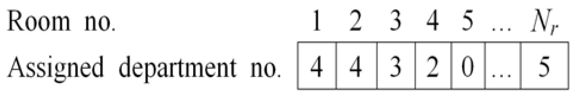
Figure 2.
Solution representation of indoor spatial allocation. The solution can be represented as a vector of Nr dimensions. The assigned department number of zero indicates that the room is not assigned to any department.
Figure 2.
Solution representation of indoor spatial allocation. The solution can be represented as a vector of Nr dimensions. The assigned department number of zero indicates that the room is not assigned to any department.

Figure 3.
Swap move of the local search.

Figure 4.
Indoor connective map of the office building in the case study.
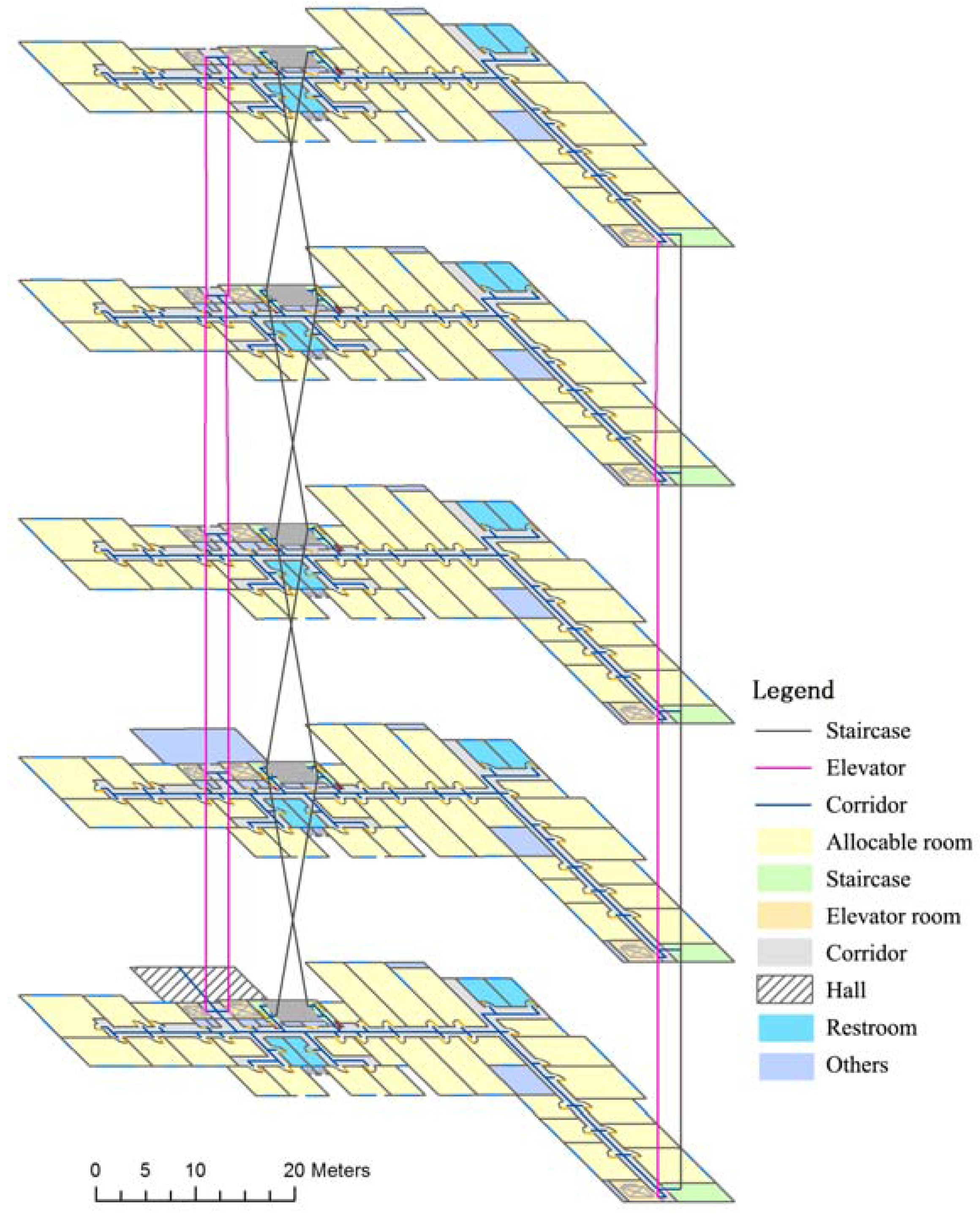
Figure 5.
The spatial representation of the multiple ant colony optimization (MACO) solution.

Figure 6.
The plans of two floors in which the departments in red ovals are not spatially aggregate.
Figure 6.
The plans of two floors in which the departments in red ovals are not spatially aggregate.

Figure 7.
Comparison of the objective function value gap from MACO without using one of these strategies and each strategy’s computation time.
Figure 7.
Comparison of the objective function value gap from MACO without using one of these strategies and each strategy’s computation time.
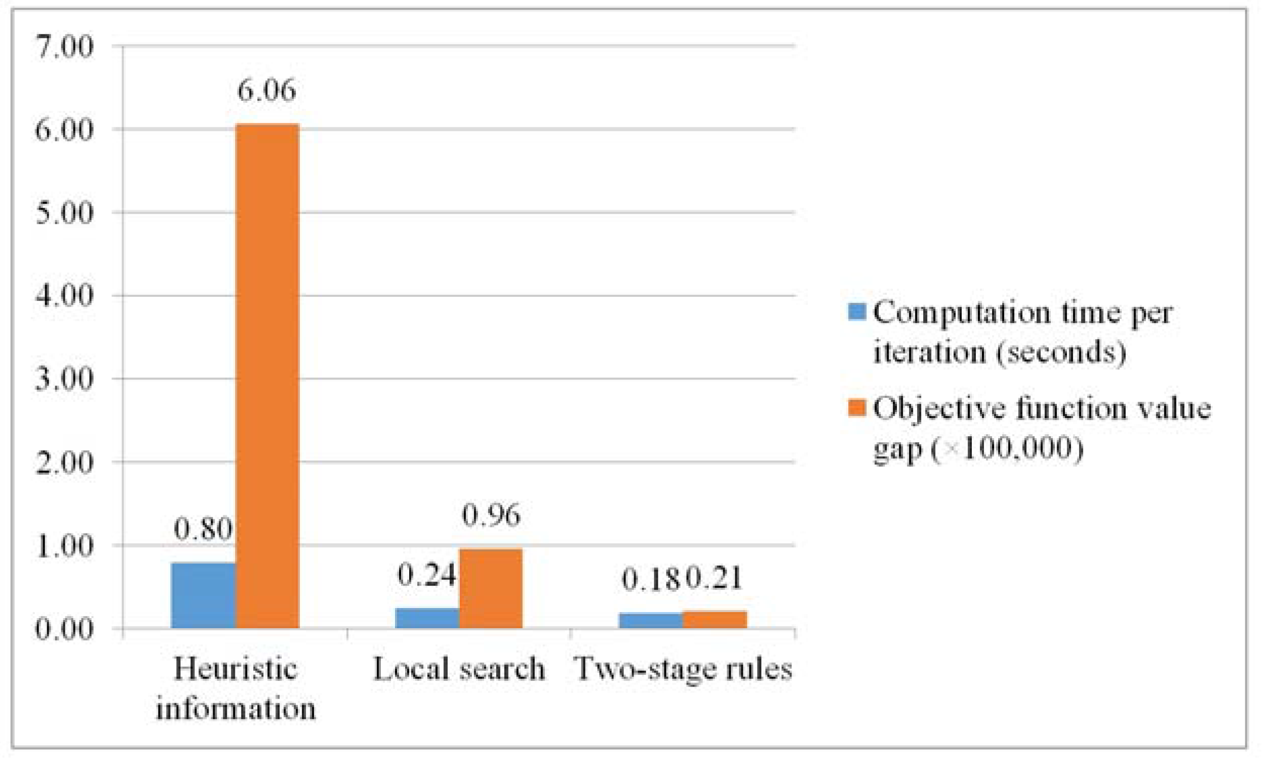
Figure 8.
Best-so-far solutions during 500 iterations. MACO and ACO-1 stopped at the 383rd and 257th iteration, respectively, because of the convergence condition: the current-best solution is the best-so-far solution for ten successive times.
Figure 8.
Best-so-far solutions during 500 iterations. MACO and ACO-1 stopped at the 383rd and 257th iteration, respectively, because of the convergence condition: the current-best solution is the best-so-far solution for ten successive times.

Figure 9.
Visualization of random generated indoor spatial data. The circles of different colors and sizes represent the allocable rooms of different areas. The numerical labels are the rooms’ area with a unit of square meters.
Figure 9.
Visualization of random generated indoor spatial data. The circles of different colors and sizes represent the allocable rooms of different areas. The numerical labels are the rooms’ area with a unit of square meters.


Table 1.
The mathematic symbols in indoor room optimal allocation.
| Mathematic Symbol | Description |
|---|---|
| Office departments | |
| Allocable rooms | |
| Each office department’s demand, the minimum working area | |
| The area of each allocable room | |
| Department type—business departments | |
| Department type—public departments | |
| The number of public departments | |
| The number of business departments | |
| The number of building exits | |
| The number of allocable rooms | |
| The public departments | |
| The business departments | |
| Indoor spatial connectivity cost between two different rooms | |
| The allocation relationship between room and department . If room is assigned to department , ; otherwise, . |
Table 2.
The mathematic symbols in evaluating the heuristic information.
| Mathematic Symbols | Descriptions |
|---|---|
| Room number | |
| , | Department number |
| The department that room is assigned to | |
| , all the rooms that are assigned to department | |
| , all the rooms that have been allocated | |
| The type of department | |
| The heuristic information on node |
Table 3.
Computational time complexity of the objective function value calculation.
| Main Steps | Computational Complexity |
|---|---|
| Calculating using Formula (1) | |
| Calculating using Formula (2) | |
| Calculating using Formula (3) |
Table 4.
Computational time complexity of ants’ behaviors in each iteration.
| Main Steps | Computational Complexity | |
|---|---|---|
| For the first ant colony | Determine the optimal order of allocating departments | |
| Updating pheromone | ||
| For the second ant colony | Calculating heuristic information | |
| Assigning rooms to each department and calculating the objective function value | ||
| Applying local search to the current-best solution and calculating the objective function value | ||
| Updating pheromone | ||
Table 5.
The allocation requirements of the office building in the case study.
| Department Type | Department No. | Minimum Area (m2) |
|---|---|---|
| Public Department | 1 | 100 |
| 2 | 100 | |
| 3 | 80 | |
| 4 | 60 | |
| 5 | 100 | |
| Business Department | 6 | 100 |
| 7 | 140 | |
| 8 | 150 | |
| 9 | 180 | |
| 10 | 210 | |
| 11 | 300 | |
| 12 | 180 | |
| 13 | 260 | |
| 14 | 320 | |
| 15 | 180 | |
| 16 | 220 |
Table 6.
Parameter selection design.
| Experiment ID | ||||||
|---|---|---|---|---|---|---|
| 1 | 20 | 1 | 1 | 1 | 0.9 | 1000 |
| 2 | 20 | 3 | 3 | 3 | 0.95 | 10,000 |
| 3 | 20 | 5 | 5 | 5 | 0.99 | 100,000 |
| 4 | 20 | 7 | 7 | 7 | 0.995 | 1,000,000 |
| 5 | 20 | 9 | 9 | 9 | 0.999 | 10,000,000 |
| 6 | 40 | 1 | 3 | 5 | 0.995 | 10,000,000 |
| 7 | 40 | 3 | 5 | 7 | 0.999 | 1000 |
| 8 | 40 | 5 | 7 | 9 | 0.9 | 10,000 |
| 9 | 40 | 7 | 9 | 1 | 0.95 | 100,000 |
| 10 | 40 | 9 | 1 | 3 | 0.99 | 1,000,000 |
| 11 | 60 | 1 | 5 | 9 | 0.95 | 1,000,000 |
| 12 | 60 | 3 | 7 | 1 | 0.99 | 10,000,000 |
| 13 | 60 | 5 | 9 | 3 | 0.995 | 1000 |
| 14 | 60 | 7 | 1 | 5 | 0.999 | 10,000 |
| 15 | 60 | 9 | 3 | 7 | 0.9 | 100,000 |
| 16 | 80 | 1 | 7 | 3 | 0.999 | 100,000 |
| 17 | 80 | 3 | 9 | 5 | 0.9 | 1,000,000 |
| 18 | 80 | 5 | 1 | 7 | 0.95 | 10,000,000 |
| 19 | 80 | 7 | 3 | 9 | 0.99 | 1000 |
| 20 | 80 | 9 | 5 | 1 | 0.995 | 10,000 |
| 21 | 100 | 1 | 9 | 7 | 0.99 | 10,000 |
| 22 | 100 | 3 | 1 | 9 | 0.995 | 100,000 |
| 23 | 100 | 5 | 3 | 1 | 0.999 | 1,000,000 |
| 24 | 100 | 7 | 5 | 3 | 0.9 | 10,000,000 |
| 25 | 100 | 9 | 7 | 5 | 0.95 | 1000 |
Table 7.
Results of the orthogonal experiments. The bold numbers are the minimal value in each column in the first five rows.
Table 7.
Results of the orthogonal experiments. The bold numbers are the minimal value in each column in the first five rows.
| Statistic Criterion | ||||||
|---|---|---|---|---|---|---|
| 25.39355 | 23.14087 | 29.45160 | 24.47543 | 24.75974 | 22.22692 | |
| 25.41501 | 24.98020 | 24.56443 | 25.64599 | 24.86951 | 24.90870 | |
| 25.27312 | 25.98248 | 24.10325 | 24.59825 | 25.90307 | 26.81958 | |
| 25.10221 | 26.37223 | 24.83291 | 27.34773 | 25.52166 | 26.56158 | |
| 26.20184 | 26.90995 | 24.43355 | 25.31833 | 26.33175 | 26.86895 | |
| Range | 1.09963 | 3.76908 | 5.34835 | 2.87230 | 1.57201 | 4.64203 |
| Primary order | 6 | 3 | 1 | 4 | 5 | 2 |
| Optimal parameter value | 80 | 1 | 5 | 1 | 0.9 | 1000 |
Table 8.
Statistics of each department’s allocated rooms.
| Department ID | Room Number | Room Area (m2) | Required Area (m2) |
|---|---|---|---|
| 1 | 3 | 102 | 100 |
| 2 | 3 | 105 | 100 |
| 3 | 3 | 81 | 80 |
| 4 | 2 | 70 | 60 |
| 5 | 3 | 102 | 100 |
| 6 | 6 | 100 | 100 |
| 7 | 7 | 141 | 140 |
| 8 | 8 | 150 | 150 |
| 9 | 10 | 181 | 180 |
| 10 | 12 | 212 | 210 |
| 11 | 12 | 303 | 300 |
| 12 | 10 | 181 | 180 |
| 13 | 11 | 261 | 260 |
| 14 | 13 | 320 | 320 |
| 15 | 8 | 182 | 180 |
| 16 | 13 | 220 | 220 |
| 0 * | 21 | 364 | - |
Note: * A department ID of zero refers to the unallocated rooms.
Table 9.
Comparison of the exchange trials while validating the optimality of the solution generated by MACO. The bold numbers are the minimal value among all comparisons.
Table 9.
Comparison of the exchange trials while validating the optimality of the solution generated by MACO. The bold numbers are the minimal value among all comparisons.
| Comparison | Department Numbers that Rooms Are Assigned to | Objective Value | ||||||
|---|---|---|---|---|---|---|---|---|
| The optimal allocation | 4 | 6 | 4 | 7 | 2.7073 | 14.733 | 1.3877 | 18.828 |
| Exchange trials 1 | 6 | 4 | 4 | 7 | 2.7029 | 14.762 | 1.3877 | 18.853 |
| Exchange trials 2 | 4 | 6 | 7 | 4 | 2.7044 | 14.749 | 1.3877 | 18.841 |
| Exchange trials 3 | 6 | 4 | 7 | 4 | 2.7000 | 12.778 | 1.3877 | 18.865 |
Table 10.
Comparison of the improved strategies.
| Experiment ID | Solution Construction | Local Search | Transition Probability | |
|---|---|---|---|---|
| Two-Colony Strategy | Pheromone | Heuristic Information | ||
| MACO | √ | √ | √ | √ |
| ACO-1 | √ | √ | √ | × |
| ACO-2 | √ | × | √ | √ |
| ACO-3 | × | √ | √ | √ |
Table 11.
Statistical results of different strategies’ comparison experiments. The bold numbers are the minimal objective function value among all comparable algorithms.
Table 11.
Statistical results of different strategies’ comparison experiments. The bold numbers are the minimal objective function value among all comparable algorithms.
| Experiment ID | Best Objective Function Value | Average Objective Function Value | Standard Deviation | Average Computation Time Per Iteration (Seconds) |
|---|---|---|---|---|
| MACO | 18.82804 | 19.74889 | 0.46364 | 2.6952 |
| ACO-1 | 24.83096 | 25.81269 | 0.60610 | 1.8989 |
| ACO-2 | 19.73300 | 20.71029 | 0.58900 | 2.4516 |
| ACO-3 | 19.12111 | 19.95435 | 0.78379 | 2.5103 |
Table 12.
Random generated allocation requirements data.
| Dataset ID | Public Department | Business Department | ||
|---|---|---|---|---|
| Department No. | Minimum Area (m2) | Department No. | Minimum Area (m2) | |
| A | 1 | 15 | 1 | 30 |
| 2 | 20 | 2 | 40 | |
| B | 1 | 40 | 1 | 90 |
| 2 | 40 | 2 | 70 | |
| 3 | 80 | |||
| 4 | 70 | |||
| C | 1 | 80 | 1 | 120 |
| 2 | 100 | 2 | 180 | |
| 3 | 200 | |||
| 4 | 140 | |||
| 5 | 160 | |||
Table 13.
Statistical results of the different algorithms’ comparison experiments.
| Data Set ID | Algorithm | Best Objective Function Value | Average Objective Function Value | Standard Deviation |
|---|---|---|---|---|
| A | MACO | 1.062468 | 1.230582 | 0.117381 |
| Genetic Algorithm(GA) | 1.062468 | 1.262189 | 0.104001 | |
| Particle Swarm Optimization (PSO) | 1.062468 | 1.178371 | 0.08068 | |
| B | MACO | 16.00452 | 16.68899 | 0.684466 |
| GA | 18.30258 | 21.09572 | 0.959144 | |
| PSO | 18.99274 | 20.59133 | 1.311235 | |
| C | MACO | 67.42195 | 69.78997 | 1.575588 |
| GA | 79.20612 | 89.7569 | 4.959768 | |
| PSO | 92.55909 | 98.81198 | 2.989783 |
© 2017 by the authors. Licensee MDPI, Basel, Switzerland. This article is an open access article distributed under the terms and conditions of the Creative Commons Attribution (CC BY) license (http://creativecommons.org/licenses/by/4.0/).
Share and Cite
MDPI and ACS Style
Yang, L.; Sun, X.; Zhu, A.; Chi, T. A Multiple Ant Colony Optimization Algorithm for Indoor Room Optimal Spatial Allocation. ISPRS Int. J. Geo-Inf. 2017, 6, 161. https://doi.org/10.3390/ijgi6060161
AMA Style
Yang L, Sun X, Zhu A, Chi T. A Multiple Ant Colony Optimization Algorithm for Indoor Room Optimal Spatial Allocation. ISPRS International Journal of Geo-Information. 2017; 6(6):161. https://doi.org/10.3390/ijgi6060161
Chicago/Turabian StyleYang, Lina, Xu Sun, Axing Zhu, and Tianhe Chi. 2017. "A Multiple Ant Colony Optimization Algorithm for Indoor Room Optimal Spatial Allocation" ISPRS International Journal of Geo-Information 6, no. 6: 161. https://doi.org/10.3390/ijgi6060161
Note that from the first issue of 2016, this journal uses article numbers instead of page numbers. See further details here.