Article

Topographic Spatial Variation Analysis of Loess Shoulder Lines in the Loess Plateau of China Based on MF-DFA

1
Key Laboratory of Virtual Geographic Environment of Ministry of Education, Nanjing Normal University, Nanjing 210023, China
2
School of Environment Science, Nanjing Xiaozhuang University, Nanjing 211171, China
3
Jiangsu Center for Collaborative Innovation in Geographical Information Resource Development and Application, Nanjing 210023, China
*
Author to whom correspondence should be addressed.
ISPRS Int. J. Geo-Inf. 2017, 6(5), 141; https://doi.org/10.3390/ijgi6050141
Submission received: 23 December 2016 / Revised: 26 April 2017 / Accepted: 27 April 2017 / Published: 2 May 2017

Abstract

:
The Loess Plateau in China is internationally known for its unique geographical features and has therefore been studied by many researchers. This research exploits the regional differences in the spatial morphological characteristics of Loess shoulder lines in different landform types as an important basis for geomorphological regionalization. In this study, we used ensemble empirical mode decomposition (EEMD), multi-fractal detrended fluctuation analysis (MF-DFA), and detrended cross-correlation analysis (DCCA) to analyze topographic data series extracted from shoulder lines. Loess shoulder-line land variations series data from the Suide, Ganquan, and Chunhua areas on the Loess Plateau were selected and a combination of the two above-mentioned methods was used to study land variations at these three sample sites. The results revealed differences in the topographic variations of the multi-fractal characteristics and the topographic spatial variation in the Loess shoulder line of the three sample sites. Furthermore, the extent to which the results were affected by noise and the analysis scale differed among the three areas.

1. Introduction

The Loess Plateau of China has drawn the attention of many researchers worldwide for its unique geographical condition, geomorphologic research values, loess landform feature, and its special natural and cultural landscapes [1,2]. Many previous studies about the Loess Plateau have been carried out to solve scientific problems regarding its formation process [3,4], landform shape [5,6,7], gully development [8,9,10], soil erosion [11,12], environmental evolution [13,14] etc., and many outstanding research results have been achieved. In recent years, the development of Digital Elevation Model (DEM) applications and Geographic Information System (GIS) spatial analysis techniques has greatly promoted the study of the land surface analysis of the Loess Plateau. Digital land surface analysis has been used to extract the basic terrain derivatives (e.g., slope and aspect) [15,16] and to study complicated applications (e.g., paleo-topographic reconstruction and landform classification) [17,18,19,20,21] of the Loess Plateau. The terrain points [22,23,24], lines [25,26,27], and surfaces [28,29,30] of the Loess Plateau have been well studied in terms of extraction methods based on DEMs. However, these studies mainly focused on research with the view of developing and evaluating technologies and methods, and there is a lack of research and discussion on the role of terrain data in the study of the topography and geomorphology of the Loess Plateau. Tang et al. [1] established the theory of the slope topo-sequence, which they successfully applied to study the Loess landform. The corresponding slope topo-sequence, which showed an obvious spatial distribution, of any of the different Loess landforms could be found [31]. The topo-sequence of hypsometric integrals (HI) was applied to the loess watershed landform in an area of the Loess Plateau affected by severe soil erosion, based on a digital land surface analysis and geo-informatics method named Tupu [32]. Furthermore, an existing method has been put forward to study the spatial distribution based on the landform planation index (LPI), which is the terrain derivative extracted from DEMs [33]. In spite of the fact that these methods realized a quantitative analysis of the macroscopic differentiation rules of the Loess Plateau, these methods are not sensitive to the local topographic changes in the Loess Plateau, which cover up the local variation of the terrain.
The Loess shoulder-line is one of the most significant topographic structures in the Loess Plateau, which separates the complicated physiognomy of the plateau distinctly into positive (inter-gully area) and negative terrains (inner-gully area) (P-N terrains) in terms of the formation and topographic feature of the landforms. This shoulder-line plays important roles in the research of soil and water conservation. As the most vital boundaries, extraction methods [34] and efficient calculations [35,36] have mainly been applied to the Loess shoulder lines in many studies. Few researchers have applied the quantitative index of the shoulder lines to study the spatial distribution of the Loess Plateau land at present. The shoulder lines formed and developed at the slope scale, meandering in the whole watershed, and carved out the spatial pattern of Loess gullies and Loess tableland, Loess ridges, and Loess hills. The regional difference in the spatial morphological characteristics of Loess shoulder lines in different landform types has become an important basis for geomorphological regionalization.
Fractal theory has been used to address the limitation of traditional quantitative methods on geomorphic features, and has opened up a new approach to generally describe the geomorphic features of a drainage basin and its geomorphic evolution [37,38]. More specifically, fractal theory has provided a way to quantitatively describe self-similar or self-affine landforms [39]. The classic application of fractals to geomorphology focused on line elements such as coastlines, rivers, and faults [18]. Based on grid DEMs, the fractal dimension was shown to characterize more than mere terrain “irregularity” or “roughness” [40]; instead, it can also be employed to describe the changes in the variability of the topography in relation to the distance [41]. The relationship between the fractal parameters and the physical processes needs further research. For a loess landform, the fine fractal structure of a single watershed varies for different landform types and developmental processes. Thus, an analysis of the geometric singularity distribution of loess shoulder lines in different loess landforms to obtain the fractal parameters of these shoulder lines could provide theoretical and methodological support for further research on scientific and reasonable classification of loess geomorphic regions.
The research described in this paper is based on elevation data, which was obtained from the actual direction of the curve at a certain distance along shoulder lines extracted from DEMs. The elevation data, as with most time series data, also consist of nonlinear and non-stationary data capable of reflecting the topographic spatial variation and relief of the area surrounding the shoulder lines. The main difference between the time series data and elevation data is that the two kinds of data are based on the time and sampling distance as independent variables, respectively. Due to a high degree of similarity within time series, it is feasible to use the elevation sampling data of shoulder lines to apply to land surface analysis.
In this study, we use the multi-fractal detrended fluctuation analysis (MF-DFA) [42] developed in recent years to study topographic data series extracted from shoulder lines. MF-DFA has successfully been applied to fields as diverse as finance and stock markets [43,44,45], seismicity [46,47,48], mineral grade detection [49], climate change [50,51,52,53,54], traffic flow [55,56], speech signal characteristics [57], plant species identification [58], air pollution [59,60], and heart rate dynamics [61]. It is very valuable to introduce this method into the analysis of shoulder-lines. In this study, MF-DFA can distinguish different landform types of local or global changes of the land surface features.
This research mainly focuses on the introduction of the multi-fractal spectrum exponent and Hurst exponent in order to describe the topographic variation law of different landform types that can reflect the overall macro- and local micro-pattern of the land surface of the Loess Plateau. The research results provide quantitative information in support of the loess landform classification.

2. Materials and Methods
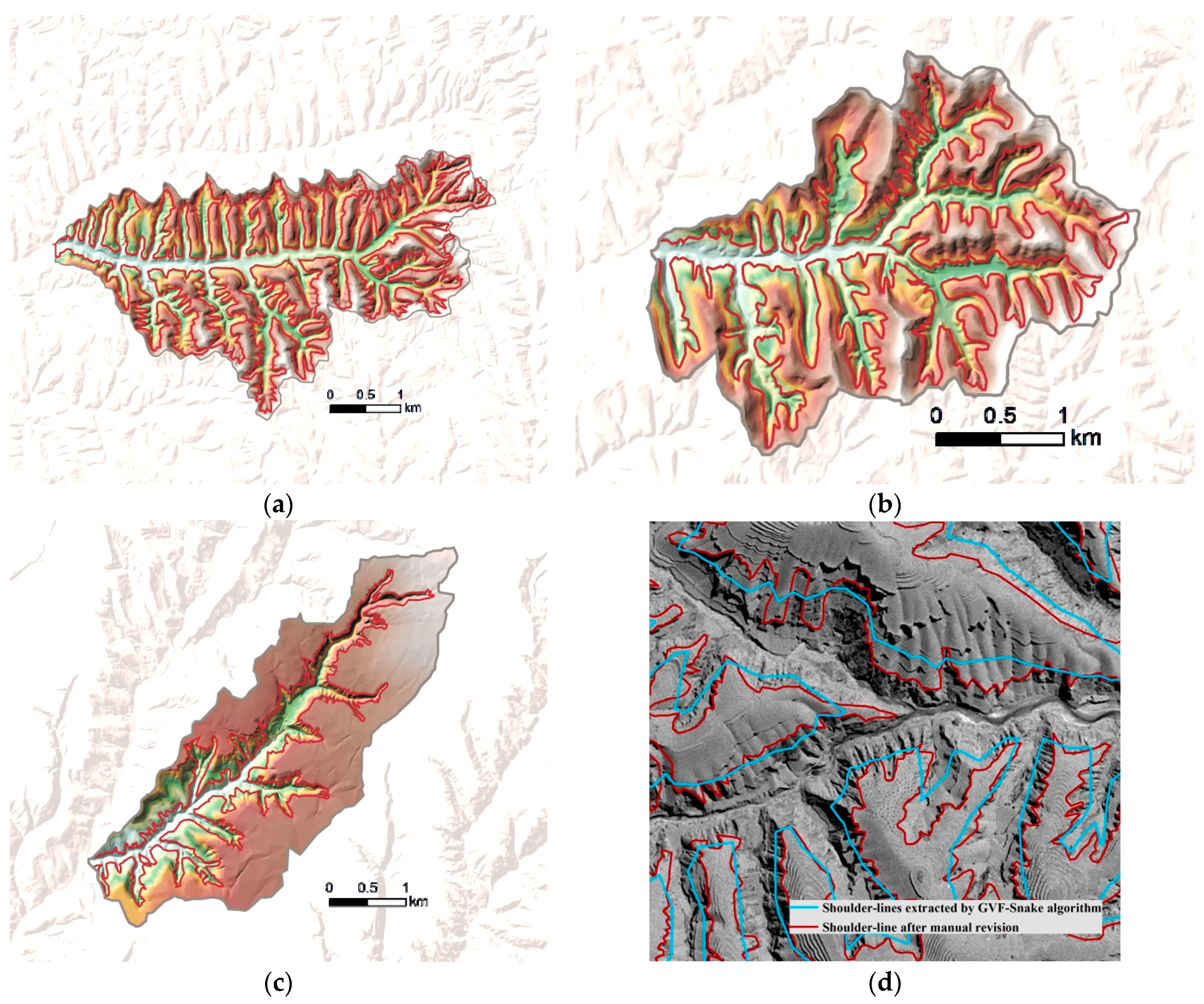
2.1. Study Area

The hilly area of the Loess Plateau of China was taken as the study area. This area was developed on a base of ancient landform consisting of Mesozoic bedrock. The Cenozoic laterite and Loess layers are cut by the flow of water, with soil erosion forming the complex gully systems. The selected area contains three types of landform: loess tableland, loess ridge, and loess hill, which are studied by our proposed method to understand their distributions and differences. Distinguishing these differences required the study sites to be confined to those with the most typical geomorphologic characteristics and without a mixture of landforms. Therefore, three sample areas were selected: (1) loess hill; (2) loess ridge; and (3) loess tableland. Geographic descriptions of each of the sample sites are provided in Table 1.

2.2. Topographical Data

All data used in this study are from the revised shoulder lines of these three sites and were extracted by DEMs with a resolution of 5 m (Figure 1). The DEMs used in this study were obtained from the National Administration of Surveying, Mapping, and Geoinformation of China, and were generated from the 1:10,000 topographic maps with a 1 m contour interval. Firstly, the paper topographic maps were drawn by ground-based surveying and then scanned into the computer with a geometric correction. Then the contour lines were digitalized and interpolated into a triangulated irregular network (TIN). Finally, the grid DEMs were interpolated by the TIN after ordinary manual editing in TIN to correct the mistakes. The shoulder line delineation could be achieved by a manual interpretation process with the automatic result derived by DEMs since the error of automatic results may lead to wrong analytic conclusions. Automatic extraction could be performed by using the GVF Snake algorithm [25]. Among the direction of the shoulder lines, elevation series were sampled with 5-m distance intervals. The number of elevation series in the three sites are 16,000 (Suide), 10,000 (Ganquan), and 7000 (Chunhua).

2.3. Methods

2.3.1. EEMD

Ensemble empirical mode decomposition (EEMD) is an adaptive analysis method for time series proposed by Wu [62], and is performed with the assistance of data noise. The addition of white noise to the signal to be decomposed allows the combination of signal and noise to be regarded as a whole, and then the Intrinsic Mode Functions (IMFs) with modal consistency can be obtained. Since the distribution of the white noise spectrum is uniform, the signals of different scales are automatically distributed to the appropriate reference scale when the signals are added to the white noise, which has a background with the same time-frequency distribution. Because the mean value of this noise is zero, noise of different frequencies will cancel each other after multiple averaging operations, and the result of the integrated mean can be directly used as the final result. The algorithm can be described as follows:
Step 1: Add white noise to the signal to be decomposed
X ( t ) = x ( t ) + n ( t )
where x(t) is the true signal and n(t) is the noise.
Step 2: Perform the EMD decomposition into a series of IMFs c j using the signals with noise
X ( t ) = j 1 m c j + r m
where r m is the residue of data X(t), after m number of IMFs are extracted.
Step 3: Repeat Steps 1 and 2 using a different type of noise each time.
X i ( t ) = x ( t ) + n i ( t )
Then decompose
X i ( t ) = j 1 m c i , j + r i m
Step 4: Calculate the mean value of the IMFs
c j = 1 N i 1 N c i , j    r m = 1 N i 1 N r i , m
The final result is obtained
X ( t ) = j 1 m c j + r m
Each IMF component obtained by the decomposition, irrespective of whether it is pure noise or the original sequence component with a clear physical significance, can be judged by a Monte-Carlo significance test proposed by Wu et al. [63]. IMFs that cannot pass the test with a confidence limit level of 99% can be seen as noise. Here, it is important to note that the noise in this particular situation (referring to the local errors in DEMs caused by sampling or some abnormal data) is totally different from the white noise used in EEMD (which is simply a mathematic support for data decomposition). Finally, all remaining IMFs are reconstructed into an entirely new data series and the fractal characteristics analyzed by the following MF-DFA method.

2.3.2. MF-DFA

The MF-DFA is an effective measure to reflect the developmental process of a system [42]. For the sum standardization of the fixed length time series, the MF-DFA method consists of six steps. The first three steps are essentially the same as in conventional DFA methods. Suppose that { x i } is a numeral series of length N, and this series obeys some compact support, i.e., xi = 0 means an insignificant fraction of the values only. The procedure of the MF-DFA method is as follows:
Step 1: Calculate the cumulative difference sequence of { x i }
Y ( i ) = k = 1 i [ x k < x > ]   i = 1 , 2 , , N
where <x> is the mean value of {x}.
Step 2: Apply backward division of the series Y ( i ) into N s = int ( N / s ) individual segments with an equal length scale s. Generally, there will remain a short part at the end of the series since the length N of the series is often not a multiple of the given scale s. Therefore, a forward division procedure should be repeated so that 2Ns segments can be obtained altogether.
Step 3: Calculate the local trend for each 2Ns segments by the least-squares procedure. Then determine the variance
F 2 ( s , p ) = 1 s i = 1 s { Y [ ( p 1 ) s + i ] y p ( i ) } 2   ( i = 1 ,   2 ,   N s )
F 2 ( s , p ) = 1 s i = 1 s { Y [ N ( p N s ) s + i ] y p ( i ) } 2   ( i = N s + 1 ,   N s + 2 ,   ,   2 N s )
where y p (i) is the fitting polynomial of segment p, p is the number of segments, s is the length scale and, and F is the variance.
Step 4: Calculate the qth order fluctuation function by averaging over all segments.
F q ( s ) = { 1 2 N s p = 1 2 N s [ F 2 ( s , p ) ] q 2 } 1 q   ( when   q   is  any real number that is not zero )
F q ( s ) = exp { 1 4 N s p = 1 2 N s ln [ F 2 ( s , p ) ] }   ( when   q = 0 )
Step 5: Use several different q to determine the scaling exponent of fluctuation function F q ( s ) . If there is long range correlation in series { x i } , F q ( s ) will exhibit an impact of power law relationship on length scale s, i.e.,
log F q ( s ) = log C + H q log s
where C is a constant, Hq is the qth scaling exponent of fluctuation function, i.e., the Hurst index. Since the Hurst exponent Hq can only measure the fluctuation of an elevation series from a global aspect, the local fluctuation trend could be indicated by the local Hurst exponent Ht. Ht could be estimated by performing the Hq calculation procedure in a local series segment around the given series location. Compared with Hq, Ht takes advantage of identifying the instant structural changes in the elevation series.
Step 6: Calculate the qth mass exponent tq, the qth singularity exponent hq and qth singularity dimension Dq. In Equation (7), tq is another measurement for scaling exponents and Hq is the Hurst index, and the relationship between these two parameters is as below,
Tq = q × Hq − 1
The mass exponent tq could be applied for estimating the qth singularity exponent hq and the qth singularity dimension Dq as below:
h q = d t q d q
D q = t q q 1
where hq is the singularity strength, used to describe the singularity degree of each interval in the time series.
Another way to characterize a multi-fractal series is Δ h q , which can be defined as below,
Δ h q = h q m a x h q m i n
where the maximum and minimum values of hq are expressed by h q m a x and h q m i n , respectively. Since the multi-fractal spectrum has either a left or a right truncation when using a pair of the qth-order of negative and positive values to generate the Hurst exponent, the width of the multi-fractal spectrum, Δ h q can indicate the homogeneity of the time series variation. A long tail to the left of the multi-fractal spectrum indicates that the series has a multi-fractal structure insensitive to local fluctuations with small magnitudes, whereas a long tail to the right indicates that the series has a multi-fractal structure insensitive to local fluctuations with large magnitudes. The larger Δ h q , the more uneven the time series distribution is reflected, and the more obvious the multi-fractal feature. The above statistical and analysis work was carried out by using the software MATLAB2014 [64].

2.3.3. DCCA

In the MF-DFA method, the length scale s is an important parameter for analysis. The scale effect assessment between the local Hurst exponent Ht and the elevation sequence is achieved by introducing a well-used method for long-term cross-correlations investigation [65], detrended cross-correlation analysis (DCCA). The procedure of the DCCA method consists of the following four steps:
Step 1: Determine the new profiles from two series, Ht series { x i } and elevation sequence { y i } .
x k = i = 1 k ( x i x ¯ ) ,   y k = i = 1 k ( y i y ¯ )   k = 1 , 2 , , N
Step 2: Similar to Step 2 in the MF-DFA method, divide the profiles { x k } and { y k } into n = 2Ns non-overlapping segments with equal length n.
Step 3: Calculate the detrended covariance as below:
F ( n ) i = 1 N n [ 1 n 1 k = i i + n ( x k x ˜ k , i ) ( y k y ˜ k , i ) ]
where x ˜ k , i and y ˜ k , i are local fitted (least-squares fit) trends of each of the divided segments. If F(n) behaves as a power-law function of n , i.e.,
F ( n ) n α
The cross-correlation exponent α can be measured by the slope of the log–log plot between F(n) and n. If α > 0.5, the long-term cross-correlations between two series are persistent, and vice versa. If α = 0.5, there is a non-cross-correlated relationship between the two series, namely a change in one series has no effect on the behavior of the other series.

3. Results

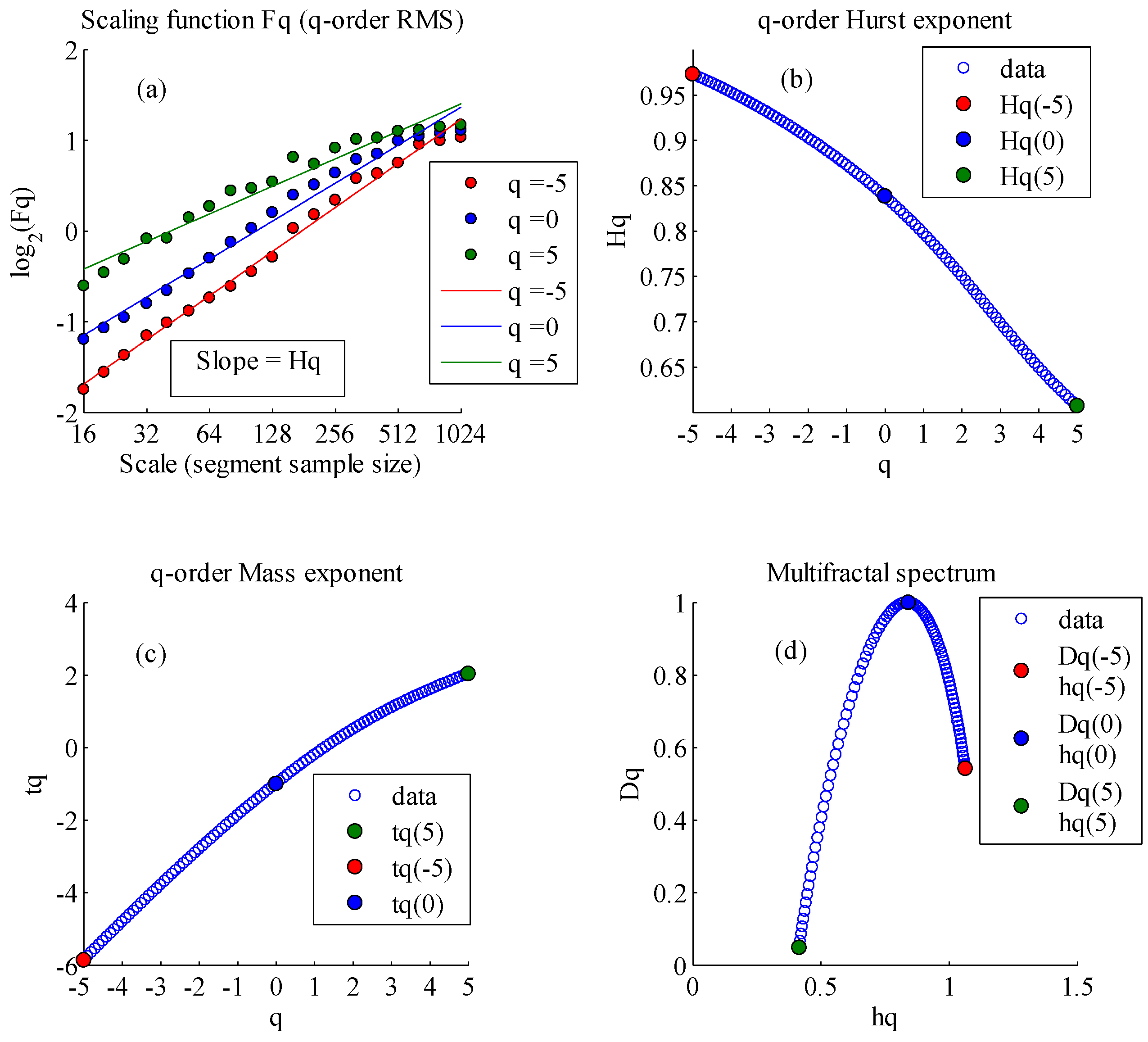
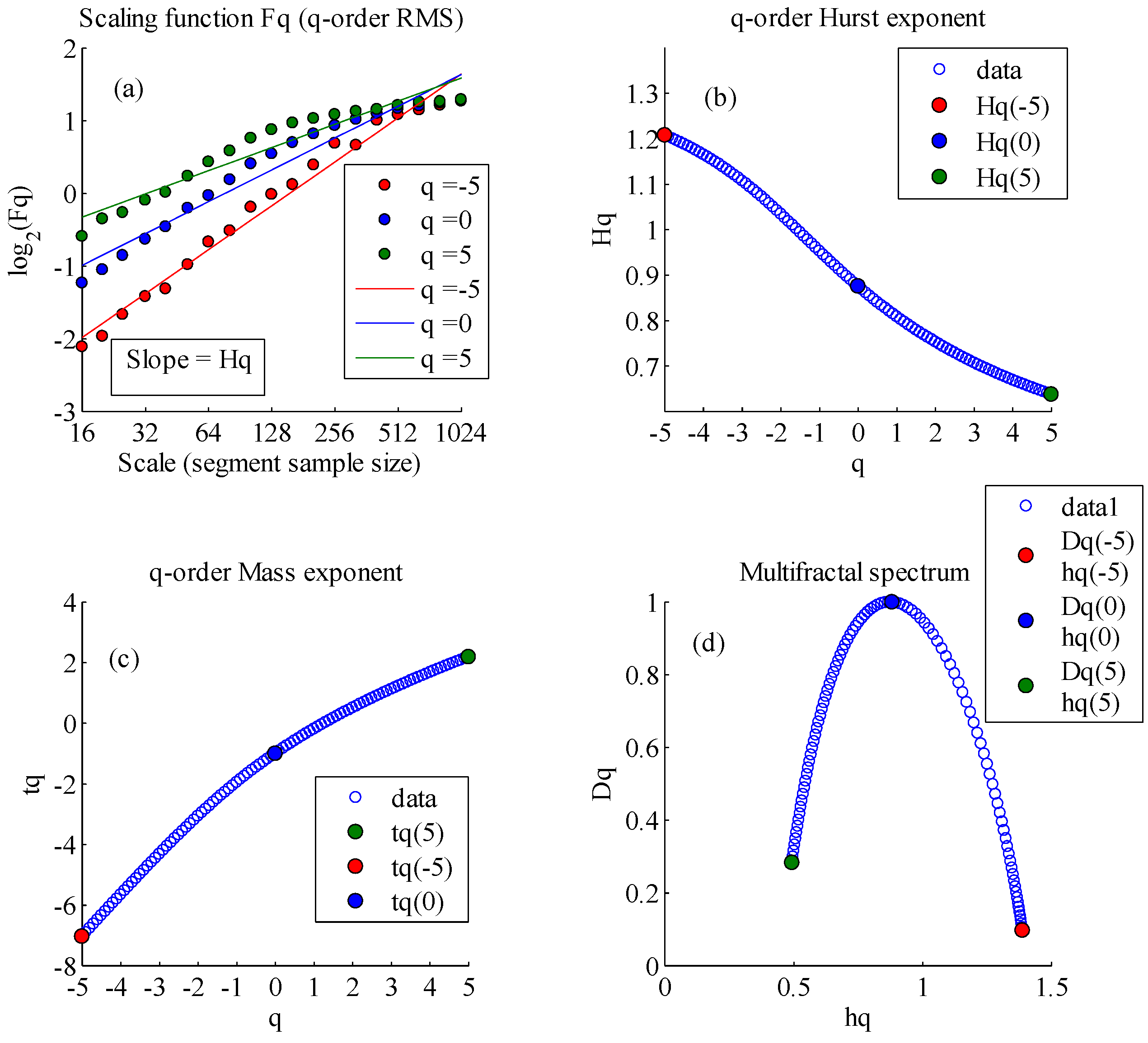
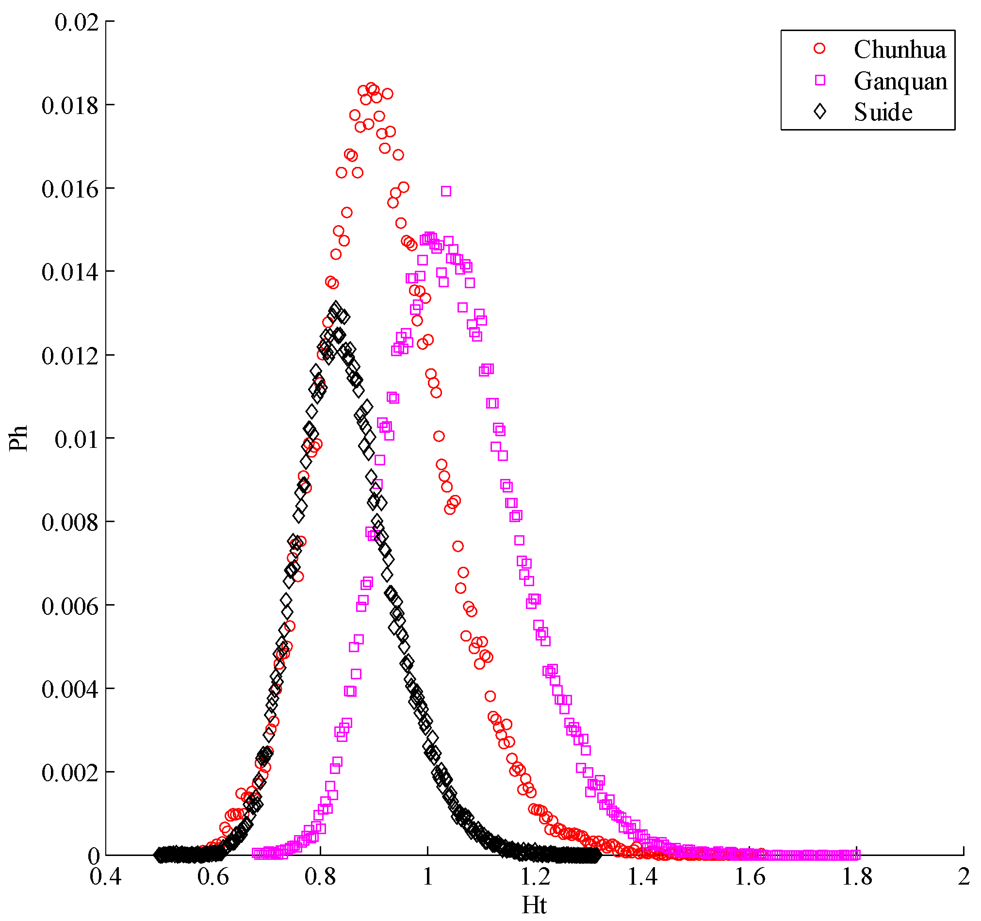
3.1. Multi-Fractal Analysis of Loess Shoulder Line

Figure 2a, Figure 3a and Figure 4a show the q-order scaling function F(q) of the study sites. According to Equations (7)–(9), the tendency by the least-squares method between the scaling function and the scale can be simulated by MATLAB software. Here, q is set to −5, 0, and 5; the scale is 16 to 1024; and the scaling function uses 2 as the basis of the logarithm. From the figures, we can see an increase in the trend between F(q) and q, and a decrease in the trend between H(q) and q. Therefore, we can conclude that the elevation series of the Loess shoulder line has a multi-fractal characteristic.
Figure 2b, Figure 3b and Figure 4b show the q-order Hurst exponents of each of the study sites according to Equation (10). We see a clear decrease in the trend between Hq and q, which confirms our argument that the elevation series of the Loess shoulder line has a multi-fractal characteristic. For the sample series, when q increases from −5 to 5, Hq of Suide decreases from 0.9729 to 0.6069, with the extent 0.366; Hq of Ganquan decreases from 1.2078 to 0.6375, with the extent 0.570; and Hq of Ganquan decreases from 1.0717 to 0.6669, with the extent 0.4048. Thus, Hq of all three areas are significantly not constant values, which reflect the strong multi-fractal characteristic. The range of Hq has a maximum value in Ganquan and a minimum value in Suide, which shows that the multi-fractal strengths of the three sites are different (Ganquan > Chunhua > Suide). In addition, in Suide and Chunhua, when q is at (−5, 5), Hq is at (0.5, 1), which indicates that the elevation series of Loess shoulder-lines has long-range correlation. This is also valid for Ganquan when q is at (−2.3, 5).
Figure 2c, Figure 3c and Figure 4c show the t-tq relationship of the three areas. We can see a clear increasing trend between tq and q, where tq is the upper convex curve. Thus, there is a nonlinear relationship between tq and q, which further confirms the multi-fractal characteristics of the Loess shoulder line [66,67]. The higher nonlinearity of the tq curves is translated into a wider f(a) dispersion with additional pronounced multi-fractal characteristics.
Figure 2d, Figure 3d and Figure 4d shows the Dqhq relationship of the three sites according to Equation (12). All of the bell curves in Figure 2d, Figure 3d and Figure 4d indicate strong multi-fractal characteristics. The top of the multi-fractal spectrum of Ganquan in Figure 3d and Table 2 is relatively flat (the spectrum width Δ h q is 0.8945), which shows that the elevation sampling data exhibit considerable fluctuation and non-uniform distribution. Contrary to this, the plots of Suide and Chunhua are relatively sharp (the spectrum widths Δ h q are 0.6479 and 0.6852), which shows a gentle fluctuation and uniform distribution.
The Suide site is characterized by a long tail to the left in its multi-fractal spectrum (Figure 2d), which is indicative of strong soil erosion in Loess positive and negative terrains. For the Chunhua site, the multi-fractal spectrum (Figure 4d) displays a long tail to the right, which shows that the elevation sampling data sequence changes gently, and that the changes in the land surface along the shoulder line are relatively small due to its relatively weak soil erosion. In Ganquan, Figure 3d shows that the multi-fractal spectrum has an approximately symmetrical shape without obvious tails to the left or right, which indicates that the elevation sampling data sequence of the shoulder line in Ganquan varies, and the land surface changes are uneven in some areas along the shoulder line and gentle in other areas.

3.2. Spatial Variation of Loess Shoulder Line

Two scales were selected to analyze the spatial distribution of the Hurst exponent. Figure 5a is the normalization result of the elevation sampling data sequence, Figure 5b is Ht with scale = 7, and Figure 5c is Ht with scale = 17. In Figure 5b,c we can see that, when scale = 7, the maximum Ht is 1.3165 (Pn = 8020), the minimum is 0.5467 (Pn = 11800), and the mode value is 0.8292; when scale = 17, the maximum Ht is 1.1736 (Pn = 8020), the minimum is 0.5082 (Pn = 11,800), and the mode value is 0.8292. The minimum value indicates that the land there is fractured while the maximum is gentle. It should be noticed that the extreme point of Ht on both scales is the same, because the scale has little effect on the analysis in the case of Suide, or probably because, at Suide, the land surface of the Loess shoulder line is fractured but has an undulating land topography distribution.
Figure 6a–c shows the results for Ganquan. In Figure 6b,c we can see that, when scale = 7, the maximum Ht is 1.8004 (Pn = 3900), the minimum is 0.6799 (Pn = 10,200), and the mode value is 1.035; and when scale = 17, the maximum Ht is 1.5420 (Pn = 2100), the minimum is 0.6838 (Pn = 1000), and the mode value is 1.035. The extreme point of Ht on both scales is totally different. This may be due to the fact that the scale has a strong effect on the analysis in Ganquan, which indicates that land morphology features vary unevenly.
Figure 7a–c shows the result for the Chunhua site. In Figure 7b,c we can see that, when scale = 7, the maximum Ht is 1.5751 (Pn = 1500), the minimum is 0.5807 (Pn = 6000), and the mode value is 0.8963; and when scale = 17, the maximum Ht is 1.3978 (Pn = 2700), the minimum is 0.5996 (Pn = 3400), and the mode value is 0.8963. The local Hurst exponent is mostly greater than the mode, while the extreme point of Ht of both scales is similar in that it is totally different, this may be due to the strong effect of the scale on the analysis of the Chunhua site, which indicates that the land morphology features are distributed unevenly.

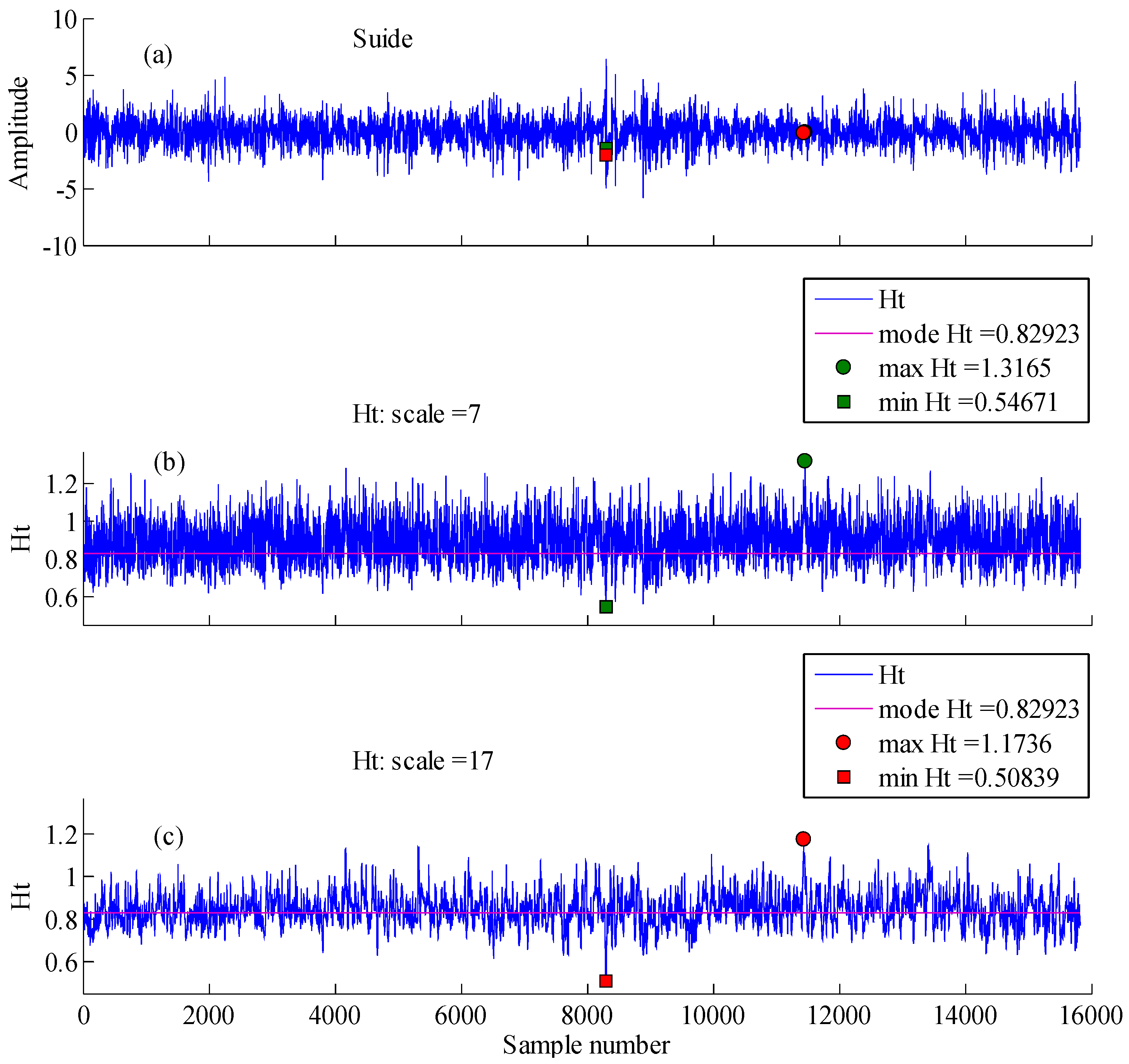
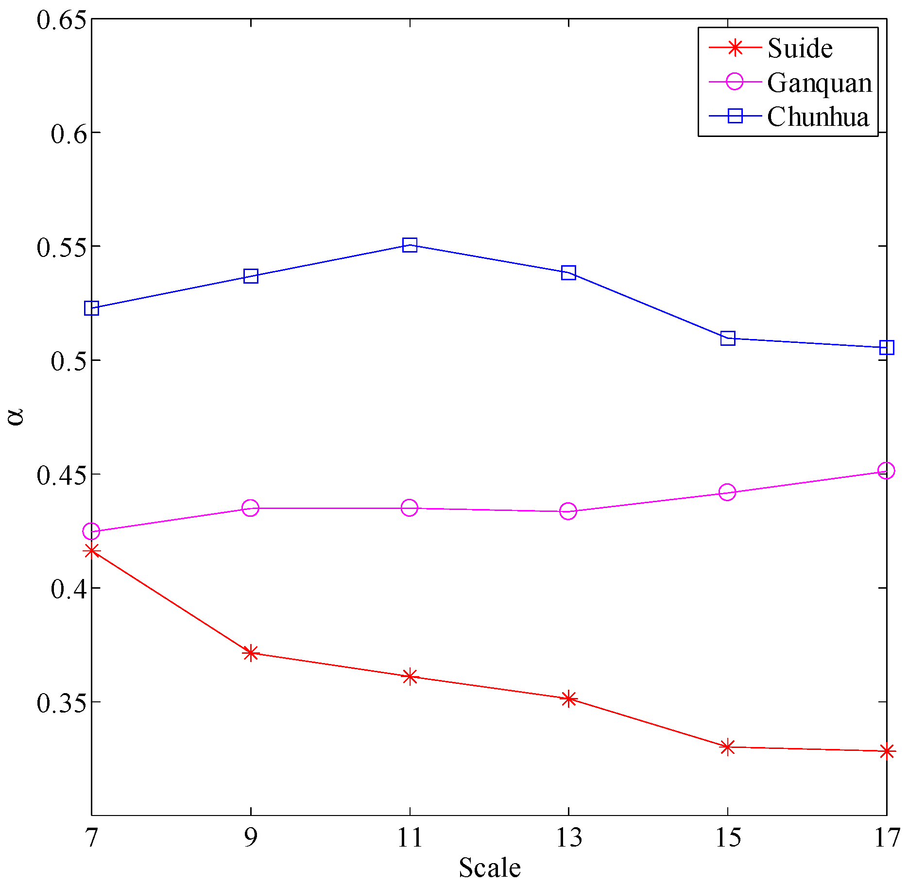
3.3. Scale Effect of Loess Shoulder-Line Topographic Variation

Figure 8a,b shows that the correlation coefficient α of the loess shoulder-line topography and local Hurst exponent of topographic variation of the Suide study site for the analysis of scale 7 and 17 are relatively small, i.e., 0.4163 and 0.3283, respectively. The DCCA parameter α decreases with increasing analysis scale, which indicates the analysis scale to loess shoulder-line topographic variation is not affected. In the different analysis scales, the DCCA correlation coefficient α of the Suide site is less than that of the Ganquan and Chunhua study sites. In all the analysis scales, the highest correlation coefficient is 0.4163, and the best analysis scale is 7 for the Suide study site. All of the DCCA correlation coefficients α are very low for the Suide site and this suggests that the local Hurst exponent is not reliable for representing the loess hill land surface variation. Figure 8c,d shows that the DCCA correlation coefficient α in the analysis scale 7 and 17 are 0.4246 and 0.4512, respectively, for the Ganquan study site. In this case, the DCCA parameter α increases when the analysis scale increases. This indicates the reliability of the local Hurst exponent that reflects the loess ridge land surface variation. For the Ganquan site, the optimal analysis scale is scale 17 when using the local Hurst exponent to describe the topographic variation. Figure 8e,f shows that the correlation coefficient α is more than 0.5 for the Chunhua site, at the analysis scale 7 and 17, the values of the correlation coefficient α are 0.5229 and 0.5055, respectively. The local Hurst exponent and loess shoulder-line land variation has a relatively strong correlation in the Chuanhua site and this indicates that the local Hurst exponent is very suitable to reflect the loess tableland topographic variation. According to Figure 9, at the different analysis scales, the DCCA correlation coefficient α is the highest for the Chunhua site, for which the correlation coefficient α is different from that of the other two sites. An increase in the analysis scale first increases and then decreases the correlation coefficient α, which reaches its maximum when the analysis scale is 11, which is the best analysis scale of the Chunhua site. In the loess shoulder-line land surface analysis of loess tableland, the selection of a suitable analysis scale has a great influence on the results of land surface analysis.
Figure 10 shows the PhHt probability distribution for all study sites. As demonstrated in Figure 11, the plot of the local Hurst exponent conforms to an approximate normal distribution and the mean Ht increases in the order: Suide < Chunhua < Ganquan. This result indicates that the topographic variations are relatively smoother at the Ganquan site, and relatively steeper at the Suide site. As demonstrated in Figure 11, the standard deviation of Ht decreases in the order: Chunhua > Ganquan > Suide. This result also indicates that Ht is concentrated around the mean of the Suide site, Ht is scattered around the mean of the Ganquan site, and Ht is the most disperse around the mean of the Chunhua site.

4. Discussion

4.1. Influence Factors of Loess Shoulder-Line

The analytic result shows the MF-DFA methods achieve a much deeper understanding of the data structure than other data analysis methods. Since the multi-fractal analysis method can be successfully applied to many complex systems, it has great potential to be applied to the land surface structure of loess shoulder lines in the Loess Plateau. The influence factors and the physical meaning of the multi-fractal characteristics of the loess shoulder-line land elevation sampled must be considered to be important.
Figure 11a shows the multi-fractal spectrum obtained by MF-DFA analysis of loess shoulder-line land elevation sampling at the Chunhua, Ganquan, and Suide study sites. This figure shows that the three curves of the multi-fractal spectrum are very similar to the curve with a long tail to the right. Determining the factors causing these results is a problem worthy of further discussion with respect to the method of land surface analysis in the Loess gully areas. First, the extraction accuracy of the Loess shoulder line is one of the important factors to influence the study. Many researchers [25,26,34] have performed an in-depth study on the extraction methods and the accuracy of the Loess shoulder line. This study is based on previous researchers’ high-accuracy extraction of the Loess shoulder line in the study area and to ensure that Loess shoulder-line data can accurately reflect the topography change of the study site. The Loess shoulder-line land elevation sample data in our study is a one-dimensional elevation series, as in other research fields, such as the time series of climate change, hydrological time series, and seismic data series. There must be noise in the series data, which may be another significant factor to cause the deviation (error) in the result of the topographic analysis of the Loess shoulder line. Thus, noise filtering of the data series is very important when using the MF-DFA method to analyze the topographic changes of the Loess shoulder-line. After the noise removal process described in Section 2.3.1, the Loess shoulder-line land elevation sample series data is analyzed by the MF-DFA method. Figure 11 shows a comparison between the multi-fractal spectrum obtained before and after noise filtering, which differs completely. The results obtained with raw data without any noise removal process, displayed in Figure 11a, show the similarity of the multi-fractal characteristics of the three study sites. Figure 11b shows that the changes in the land surface of the Loess shoulder line are different for the three study sites, and that the topographic change reflected in the multi-fractal spectrum of the Loess shoulder-line is consistent with the actual terrain. A detailed description of the loess shoulder-line topographic variation at the three sites is presented in the Results Section. This is reflected in the land surface analysis of the loess shoulder line, where the noise in the data is a non-negligible impact factor.

4.2. Correlation Analysis with Other Geographical Agents

The results of Suide show that the width of the multifractal spectrum of the Suide site is 0.6479, which indicates that the internal variation of the terrain of this site is relatively uniform. This may be related to the land use type of the Suide site, which is mainly artificial terraced fields. The Suide site is characterized by a large number of artificial terraces of various types, which have a great effect on reducing the soil erosion [68]. In addition, the site also has a large number of check-dams, which also has a great effect on weakening soil erosion [69,70,71]. The check-dam intercepts a large amount of sediment from an upstream channel, and the slope in combination with the siltation of the check-dam, gradually forms a new equilibrium profile upstream, and elevates the erosion datum of its control site. The erosion energy of the upper reaches of the dam and the slope on both sides of the dam gradually decrease; therefore, the erosion effect is weakened, forcing the evolution of the small watershed to accelerate the transition into “old age.”
The results of the Ganquan site show that the multifractal spectral width is 0.8945, which indicates that the variation in terrain changes along the Ganquan site is very different and the terrain change is more intense. This may also be related to the land use type, rainfall intensity, and so on. The main land use type in the Ganquan site is grassland, but the coverage is very low, and many places are bare loess, with a weak effect on soil erosion. The average annual precipitation at the Ganquan site is ~500 mm, which is mainly concentrated in the form of heavy rain in summer, and soil erosion is very serious. Unlike the Suide site, Ganquan has few such soil and water conservation facilities. Heavy rain in summer could cause serious soil erosion, so the gullies develop very actively, resulting in the intensive terrain variation of the Ganquan site.
The results of the Chunhua site show that the multifractal spectral width is 0.6852, which indicates that the difference in terrain variation along the shoulder line is similar. The landform type of the Chunhua site is dominated by loess tableland, and the ratio of hilly to gully sites is about 8:2. Although the annual precipitation is 600.6 mm, the land use type is mainly garden and woodland, and the vegetation cover is more pronounced. In addition, the loess soil layer at the Chunhua site is thinner and the bedrock is exposed, leading to a high erosion base as well as weak soil erosion.

5. Conclusions

A multifractal, also known as a multiple fractal measure, reveals a class of complexities and singularity. A whole site with a complex fractal characteristic can be divided into many small sites with different singularities, so that the internal fine structure of the fractal can be understood more thoroughly.
Loess shoulder-line land surface variations series data from the Suide, Ganquan, and Chunhua sites were selected and the MF-DFA method was used to study the variations in these three land sites. The following conclusions were drawn. The loess shoulder-line topographic variations have strong multi-fractal characteristics at the three sites. The strongest multi-fractal characteristics were found at the Ganquan site, followed by the Chunhua site, with the weakest multi-fractal characteristics at the Suide site. The noise and analysis scale of sampling data have a strong influence on the analysis of the loess shoulder line, and the best scale values of the three areas are different, namely 7, 17, and 11 for the Suide, Ganquan, and Chunhua sites, respectively. The topographic spatial variations of the loess shoulder-line are mainly related to other geographic agents, such as lithology, precipitation, and land use. At the Suide site, artificial landforms (such as artificial terraces and check-dams) are the main factor; at the Ganquan site, precipitation; and at the Chunhua site, lithology. The results showed that the combination of EEMD, MF-DFA, and DCCA achieved success in revealing the terrain variations on a watershed. The results could provide theoretical and methodological support for further research on scientific and reasonable classification of loess geomorphic regions. We are optimistic about the potential use of our methods.

Acknowledgments

This work was supported by the National Natural Science Foundation of China (Nos. 41471316, 41401441, and 41671389), and a project funded by the Priority Academic Program Development of Jiangsu Higher Education Institutions No. 164320H116.

Author Contributions

Jianjun Cao conceived, designed, and performed the experiments; Jianjun Cao and Jiaming Na wrote the paper; Jilong Li contributed to the data analysis; Guoan Tang reviewed the manuscript; Xuan Fang made revision; and Liyang Xiong made revision and supervised the study. All authors read and approved the manuscript.

Conflicts of Interest

The authors declare no conflict of interest.

References

  1. Tang, G.; Li, F.; Liu, X.; Long, Y.; Yang, X. Research on the slope spectrum of the Loess Plateau. Sci. China Ser. E Technol. Sci. 2008, 51, 175–185. [Google Scholar] [CrossRef]
  2. Liu, D.; Ding, Z.; Guo, Z. Loess, Environment, and Global Change; Science Press: Beijing, China, 1991. [Google Scholar]
  3. Ding, Z.; Sun, J.; Liu, T.; Zhu, R.; Yang, S.; Guo, B. Wind-blown origin of the Pliocene red clay formation in the central Loess Plateau, China. Earth Planet. Sci. Lett. 1998, 161, 135–143. [Google Scholar] [CrossRef]
  4. Guo, Z.; Ruddiman, W.F.; Hao, Q.; Wu, H.; Qiao, Y.; Zhu, R.X.; Peng, S.; Wei, J.; Yuan, B.; Liu, T. Onset of Asian desertification by 22 Myr ago inferred from loess deposits in China. Nature 2002, 416, 159–163. [Google Scholar] [CrossRef] [PubMed]
  5. Moore, I.D.; Gessler, P.; Nielsen, G.; Peterson, G. Soil attribute prediction using terrain analysis. Soil Sci. Soc. Am. J. 1993, 57, 443–452. [Google Scholar] [CrossRef]
  6. Quine, T.A.; Govers, G.; Walling, D.E.; Zhang, X.; Desmet, P.J.; Zhang, Y.; Vandaele, K. Erosion processes and landform evolution on agricultural land—New perspectives from caesium—137 measurements and topographic—Based erosion modelling. Earth Surf. Process. Landf. 1997, 22, 799–816. [Google Scholar] [CrossRef]
  7. Zhou, Y.; Tang, G.; Yang, X.; Xiao, C.; Zhang, Y.; Luo, M. Positive and negative terrains on northern Shaanxi Loess Plateau. J. Geogr. Sci. 2010, 20, 64–76. [Google Scholar] [CrossRef]
  8. Wu, Y.; Cheng, H. Monitoring of gully erosion on the Loess Plateau of China using a global positioning system. Catena 2005, 63, 154–166. [Google Scholar] [CrossRef]
  9. Hessel, R.; van Asch, T. Modelling gully erosion for a small catchment on the Chinese Loess Plateau. Catena 2003, 54, 131–146. [Google Scholar] [CrossRef]
  10. Zhu, T. Gully and tunnel erosion in the hilly Loess Plateau region, China. Geomorphology 2012, 153, 144–155. [Google Scholar] [CrossRef]
  11. Xiubin, H.; Tang, K.; Zhang, X. Soil erosion dynamics on the Chinese Loess Plateau in the last 10,000 years. Mt. Res. Dev. 2004, 24, 342–347. [Google Scholar] [CrossRef]
  12. Fu, B.; Zhao, W.; Chen, L.; Zhang, Q.; Lü, Y.; Gulinck, H.; Poesen, J. Assessment of soil erosion at large watershed scale using RUSLE and GIS: A case study in the Loess Plateau of China. Land Degrad. Dev. 2005, 16, 73–85. [Google Scholar] [CrossRef]
  13. Wu, F.; Fang, X.; Ma, Y.; An, Z.; Li, J. A 1.5 Ma sporopollen record of paleoecologic environment evolution in the central Chinese Loess Plateau. Chin. Sci. Bull. 2004, 49, 295–302. [Google Scholar] [CrossRef]
  14. Jahn, B.-M.; Gallet, S.; Han, J. Geochemistry of the Xining, Xifeng and Jixian sections, Loess Plateau of China: Eolian dust provenance and paleosol evolution during the last 140 ka. Chem. Geol. 2001, 178, 71–94. [Google Scholar] [CrossRef]
  15. Goulden, T.; Hopkinson, C.; Jamieson, R.; Sterling, S. Sensitivity of DEM, slope, aspect and watershed attributes to LiDAR measurement uncertainty. Remote Sens. Environ. 2016, 179, 23–35. [Google Scholar] [CrossRef]
  16. Bolstad, P.V.; Stowe, T. An evaluation of DEM accuracy: Elevation, slope, and aspect. Photogramm. Eng. Remote Sens. 1994, 60, 1327–1332. [Google Scholar]
  17. Xiong, L.-Y.; Tang, G.-A.; Zhu, A.-X.; Li, J.-L.; Duan, J.-Z.; Qian, Y.-Q. Landform-derived placement of electrical resistivity prospecting for paleotopography reconstruction in the loess landforms of China. J. Appl. Geophys. 2016, 131, 1–13. [Google Scholar] [CrossRef]
  18. Bi, L.; He, H.; Wei, Z.; Shi, F. Fractal properties of landforms in the Ordos Block and surrounding areas, China. Geomorphology 2012, 175, 151–162. [Google Scholar] [CrossRef]
  19. Cheng, W.; Zhou, C.; Li, B.; Shen, Y.; Zhang, B. Structure and contents of layered classification system of digital geomorphology for China. J. Geogr. Sci. 2011, 21, 771–790. [Google Scholar] [CrossRef]
  20. Xiong, L.Y.; Tang, G.A.; Strobl, J.; Zhu, A. Paleotopographic controls on loess deposition in the Loess Plateau of China. Earth Surf. Process. Landf. 2016, 41, 1155–1168. [Google Scholar] [CrossRef]
  21. Bergonse, R.; Reis, E. Reconstructing pre-erosion topography using spatial interpolation techniques: A validation-based approach. J. Geogr. Sci. 2015, 25, 196–210. [Google Scholar] [CrossRef]
  22. Zhu, H.; Tang, G.; Qian, K.; Liu, H. Extraction and analysis of gully head of Loess Plateau in China based on digital elevation model. Chin. Geogr. Sci. 2014, 24, 328–338. [Google Scholar] [CrossRef]
  23. Tian, J.; Tang, G.-A.; Zhou, Y. Points Group of Topographical Feature Based On SOFM. In Proceedings of the 2012 2nd International Conference on Remote Sensing, Environment and Transportation Engineering (RSETE), Nanjing, China, 1–3 June 2012; pp. 1–4. [Google Scholar]
  24. Li, J.; Tang, G.-A.; Zhang, T.; Xiao, C.-C. Conflux threshold of extracting stream networks from DEMs in north Shaanxi province of Loess Plateau. Bull. Soil Water Conserv. 2007, 2, 75–78. [Google Scholar]
  25. Song, X.D.; Tang, G.A.; Li, F.Y.; Jiang, L.; Zhou, Y.; Qian, K.J. Extraction of loess shoulder-line based on the parallel GVF snake model in the loess hilly area of China. Comput. Geosci. 2013, 52, 11–20. [Google Scholar] [CrossRef]
  26. Yan, S.-J.; Tang, G.A.; Li, F.-Y.; Zhang, L. Snake model for the extraction of loess shoulder-line from DEMs. J. Mt. Sci. 2014, 11, 1552–1559. [Google Scholar] [CrossRef]
  27. Bai, R.; Li, T.; Huang, Y.; Li, J.; Wang, G. An efficient and comprehensive method for drainage network extraction from DEM with billions of pixels using a size-balanced binary search tree. Geomorphology 2015, 238, 56–67. [Google Scholar] [CrossRef]
  28. Chen, Y.-G.; Yang, C.-J.; Chen, X.-Y.; Ma, T.-W.; Wang, L.; Du, J.-Y. A new method of tree structure for analysing nested watershed shape. Geomorphology 2016, 265, 98–106. [Google Scholar] [CrossRef]
  29. Li, T.; Wang, G.; Chen, J. A modified binary tree codification of drainage networks to support complex hydrological models. Comput. Geosci. 2010, 36, 1427–1435. [Google Scholar] [CrossRef]
  30. Liu, K.; Ding, H.; Tang, G.; Na, J.; Huang, X.; Xue, Z.; Yang, X.; Li, F. Detection of catchment-scale gully-affected areas using unmanned aerial vehicle (UAV) on the Chinese Loess Plateau. ISPRS Int. J. Geo-Inf. 2016, 5, 238. [Google Scholar] [CrossRef]
  31. Li, F.; Tang, G.; Wang, C.; Cui, L.; Zhu, R. Slope spectrum variation in a simulated loess watershed. Front. Earth Sci. 2016, 10, 328–339. [Google Scholar] [CrossRef]
  32. Zhu, S.; Tang, G.A.; Li, F.; Xiong, L. Spatial variation of hypsometric integral in the Loess Plateau based on DEM. Acta Geogr. Sin. 2013, 7, 921–932. [Google Scholar]
  33. Qian, Y.; Xiong, L.; Li, J.; Tang, G. Landform planation index extracted from DEMs: A case study in Ordos platform of China. Chin. Geogr. Sci. 2016, 26, 314–324. [Google Scholar] [CrossRef]
  34. Jiang, S.; Tang, G.; Liu, K. A new extraction method of loess shoulder-line based on marr-hildreth operator and terrain mask. PLoS ONE 2015, 10, e0123804. [Google Scholar] [CrossRef] [PubMed]
  35. Jiang, L.; Tang, G.; Liu, X.; Song, X.; Yang, J.; Liu, K. Parallel contributing area calculation with granularity control on massive grid terrain datasets. Comput. Geosci. 2013, 60, 70–80. [Google Scholar] [CrossRef]
  36. Liu, K.; Tang, G.; Jiang, L.; Zhu, A.-X.; Yang, J.; Song, X. Regional-scale calculation of the LS factor using parallel processing. Comput. Geosci. 2015, 78, 110–122. [Google Scholar] [CrossRef]
  37. Gagnon, J.-S.; Lovejoy, S.; Schertzer, D. Multifractal earth topography. Nonlinear Process. Geophys. 2006, 13, 541–570. [Google Scholar] [CrossRef]
  38. Ramisch, A.; Bebermeier, W.; Hartmann, K.; Schütt, B.; Alexanian, N. Fractals in topography: Application to geoarchaeological studies in the surroundings of the necropolis of Dahshur, Egypt. Q. Int. 2012, 266, 34–46. [Google Scholar] [CrossRef]
  39. Mandelbrot, B.B. How long is the coast of Britain. Science 1967, 156, 636–638. [Google Scholar] [CrossRef] [PubMed]
  40. Xu, T.; Moore, I.D.; Gallant, J.C. Fractals, fractal dimensions and landscapes—A review. Geomorphology 1993, 8, 245–262. [Google Scholar] [CrossRef]
  41. Chase, C.G. Fluvial landsculpting and the fractal dimension of topography. Geomorphology 1992, 5, 39–57. [Google Scholar] [CrossRef]
  42. Kantelhardt, J.W.; Zschiegner, S.A.; Koscielny-Bunde, E.; Havlin, S.; Bunde, A.; Stanley, H.E. Multi-fractal detrended fluctuation analysis of nonstationary time series. Phys. A Stat. Mech. Its Appl. 2002, 316, 87–114. [Google Scholar] [CrossRef]
  43. Lee, H.; Chang, W. Multi-fractal regime detecting method for financial time series. Chaos Solitons Fractals 2015, 70, 117–129. [Google Scholar] [CrossRef]
  44. Stošić, D.; Stošić, T.; Stanley, H.E. Multi-fractal properties of price change and volume change of stock market indices. Phys. A Stat. Mech. Its Appl. 2015, 428, 46–51. [Google Scholar] [CrossRef]
  45. Dewandaru, G.; Masih, R.; Bacha, O.I.; Masih, A.M.M. Developing trading strategies based on fractal finance: An application of MF-DFA in the context of Islamic equities. Phys. A Stat. Mech. Its Appl. 2015, 438, 223–235. [Google Scholar] [CrossRef]
  46. Chamoli, A.; Yadav, R. Multi-fractality in seismic sequences of NW Himalaya. Nat. Hazards 2015, 77, 19–32. [Google Scholar] [CrossRef]
  47. Michas, G.; Sammonds, P.; Vallianatos, F. Dynamic multi-fractality in earthquake time series: Insights from the corinth rift, Greece. Pure Appl. Geophys. 2015, 172, 1909–1921. [Google Scholar] [CrossRef]
  48. Telesca, L.; Matcharashvili, T.; Chelidze, T.; Zhukova, N.; Javakhishvili, Z. Investigating the dynamical features of the time distribution of the reservoir-induced seismicity in Enguri area (Georgia). Nat. Hazards 2015, 77, 117–125. [Google Scholar] [CrossRef]
  49. Wan, L.; Zhu, Y.; Deng, X. Multi-fractal characteristics of gold grades series in the Dayingezhuang Deposit, Jiaodong Gold Province, China. Earth Sci. Inf. 2015, 8, 843–851. [Google Scholar] [CrossRef]
  50. Liu, D.; Luo, M.; Fu, Q.; Zhang, Y.; Imran, K.M.; Zhao, D.; Li, T.; Abrar, F.M. Precipitation complexity measurement using multi-fractal spectra empirical mode decomposition detrended fluctuation analysis. Water Resour. Manag. 2016, 30, 505–522. [Google Scholar] [CrossRef]
  51. Shao, Z.-G.; Ditlevsen, P.D. Contrasting scaling properties of interglacial and glacial climates. Nat. Commun. 2016, 7, 10951. [Google Scholar] [CrossRef] [PubMed]
  52. Mali, P. Multi-fractal characterization of global temperature anomalies. Theor. Appl. Climatol. 2015, 121, 641–648. [Google Scholar] [CrossRef]
  53. Lana, X.; Burgueño, A.; Martínez, M.; Serra, C. Monthly rain amounts at Fabra Observatory (Barcelona, NE Spain): Fractal structure, autoregressive processes and correlation with monthly western Mediterranean Oscillation index. Int. J. Climatol. 2016, 37, 1557–1577. [Google Scholar] [CrossRef]
  54. Lana, X.; Burgueño, A.; Martínez, M.; Serra, C. Complexity and predictability of the monthly western Mediterranean Oscillation index. Int. J. Climatol. 2016, 36, 2435–2450. [Google Scholar] [CrossRef]
  55. Yin, Y.; Shang, P. Multiscale multi-fractal detrended cross-correlation analysis of traffic flow. Nonlinear Dyn. 2015, 81, 1329–1347. [Google Scholar] [CrossRef]
  56. Xu, M.; Shang, P.; Xia, J. Traffic signals analysis using qSDiFF and qHDiFF with surrogate data. Commun. Nonlinear Sci. Numerical Simul. 2015, 28, 98–108. [Google Scholar] [CrossRef]
  57. Zhao, H.; He, S. Analysis of speech signals’ characteristics based on MF-DFA with moving overlapping windows. Phys. A Stat. Mech. Its Appl. 2016, 442, 343–349. [Google Scholar] [CrossRef]
  58. Wang, F.; Liao, D.-W.; Li, J.-W.; Liao, G.-P. Two-dimensional multi-fractal detrended fluctuation analysis for plant identification. Plant Methods 2015, 11, 1. [Google Scholar] [CrossRef] [PubMed]
  59. Zhang, C.; Ni, Z.; Ni, L.; Li, J.; Zhou, L. Asymmetric multi-fractal detrending moving average analysis in time series of PM2.5 concentration. Phys. A Stat. Mech. Its Appl. 2016, 457, 322–330. [Google Scholar] [CrossRef]
  60. Xue, Y.; Pan, W.; Lu, W.-Z.; He, H.-D. Multi-fractal nature of particulate matters (PMS) in Hong Kong urban air. Sci. Total Environ. 2015, 532, 744–751. [Google Scholar] [CrossRef] [PubMed]
  61. Bhaduri, A.; Ghosh, D. Quantitative assessment of heart rate dynamics during meditation: An ECG based study with multi-fractality and visibility graph. Front. Physiol. 2016, 7, 44. [Google Scholar] [CrossRef] [PubMed]
  62. Wu, Z.; Huang, N. Ensemble empirical mode decomposition: A noise-assisted data analysis method. Adv. Adapt. Data Anal. 2009, 1, 1–41. [Google Scholar] [CrossRef]
  63. Wu, Z.; Huang, N.E. A study of the characteristics of white noise using the empirical mode decomposition method. Proc. R. Soc. Lond. A Math. Phys. Eng. Sci. 2004, 460, 1597–1611. [Google Scholar] [CrossRef]
  64. Ihlen, E.A.F. Introduction to multifractal detrended fluctuation analysis in Matlab. Front. Psychol. 2012, 3, 1–18. [Google Scholar] [CrossRef] [PubMed]
  65. Podobnik, B.; Stanley, H.E. Detrended cross-correlation analysis: A new method for analyzing two nonstationary time series. Phys. Rev. Lett. 2008, 100, 084102. [Google Scholar] [CrossRef] [PubMed]
  66. Lee, C.K.; Ho, D.S.; Yu, C.C.; Wang, C.C.; Hsiao, Y.H. Simple multi-fractal cascade model for air pollutant concentration (APC) time series. Environmetrics 2003, 14, 255–269. [Google Scholar] [CrossRef]
  67. Lee, C.-K.; Juang, L.-C.; Wang, C.-C.; Liao, Y.-Y.; Yu, C.-C.; Liu, Y.-C.; Ho, D.-S. Scaling characteristics in ozone concentration time series (OCTS). Chemosphere 2006, 62, 934–946. [Google Scholar] [CrossRef] [PubMed]
  68. Fu, B. Soil erosion and its control in the Loess Plateau of China. Soil Use Manag. 1989, 5, 76–82. [Google Scholar] [CrossRef]
  69. Zhao, G.; Kondolf, G.M.; Mu, X.; Han, M.; He, Z.; Rubin, Z.; Wang, F.; Gao, P.; Sun, W. Sediment yield reduction associated with land use changes and check dams in a catchment of the Loess Plateau, China. Catena 2017, 148, 126–137. [Google Scholar] [CrossRef]
  70. Wei, Y.; He, Z.; Li, Y.; Zhao, G.; Mu, X. Sediment Yield Deduction from Check-dams Deposition in the Weathered Sandstone Watershed on the North Loess Plateau, China. Land Degrad. Dev. 2017, 28, 217–231. [Google Scholar] [CrossRef]
  71. Zhao, G.; Mu, X.; Han, M.; An, Z.; Gao, P.; Sun, W.; Xu, W. Sediment yield and sources in dam-controlled watersheds on the northern Loess Plateau. Catena 2017, 149, 110–119. [Google Scholar] [CrossRef]
Figure 1. Data used in this study: (a) Suide; (b) Ganquan; (c) Chunhua; and (d) comparison of the automatic extraction and manual revision (enlargement of part of the Suide site).
Ijgi 06 00141 g001
Figure 2. Multi-fractal analysis of the Loess shoulder line in the Suide site. (a) q-order scale function; (b) q-order Hurst exponent; (c) q-order mass exponent; (d) multifractal spectrum.
Ijgi 06 00141 g002
Figure 3. Multi-fractal analysis of the Loess shoulder line in the Ganquan site. (a) q-order scale function; (b) q-order Hurst exponent; (c) q-order mass exponent; (d) multifractal spectrum.
Ijgi 06 00141 g003
Figure 4. Multi-fractal analysis of the Loess shoulder line in the Chunhua site. (a) q-order scale function; (b) q-order Hurst exponent; (c) q-order mass exponent; (d) multifractal spectrum.
Ijgi 06 00141 g004
Figure 5. Hurst exponent of sampling data of shoulder line with different scales for the Suide site.(a) the standard of profile of shoulder line; (b) Ht variation in analysis scale 7; (c) Ht variation in analysis scale 17.
Ijgi 06 00141 g005
Figure 6. Hurst exponent of sampling data of shoulder line with different scales for the Ganquan site. (a) the standard of profile of shoulder line; (b) Ht variation in analysis scale 7; (c) Ht variation in analysis scale 17.
Ijgi 06 00141 g006
Figure 7. Hurst exponent of sampling data of shoulder line with different scales for the Chunhua site. (a) the standard of profile of shoulder line; (b) Ht variation in analysis scale 7; (c) Ht variation in analysis scale 17.
Ijgi 06 00141 g007
Figure 8. DCCA analysis of the local Hurst exponent of the topographic variation and loess shoulder-line elevation sample data at different scales. (a) The α of analysis scale 7 in Suide site; (b) the α of analysis scale 17 in Suide site; (c) the α of analysis scale 7 in Ganquan site; (d) the α of analysis scale 17 in Ganquan site; (e) the α of analysis scale 7 in Chunhua site; (f) the α of analysis scale 17 in Chunhua site.
Ijgi 06 00141 g008
Figure 9. Scale effects of DCCA parameters α on the local Hurst exponent of loess shoulder-line and topographic variation.
Ijgi 06 00141 g009
Figure 10. Probability distribution of the local Hurst exponent of loess shoulder-line land surface variation.
Ijgi 06 00141 g010
Figure 11. Multi-fractal spectrum of loess shoulder-line elevation sample data: (a) multi-fractal spectrum of raw data; and (b) multi-fractal spectrum of noise filtering data.
Ijgi 06 00141 g011
Table 1. Geographic description of study sites.
LandformLocationGeographic Descriptions
Loess hill110°15′00′′–110°22′30′′ E; 37°32′30′′–37°37′30′′ NLocated in Suide county, Shaanxi province with an elevation between 814 and 1188 m, an average slope inclination of 29° and 9.39 km−1 of gully destiny. The intensive soil erosion in this area characterizes the fragmented land, which have a strong self-like morphology.
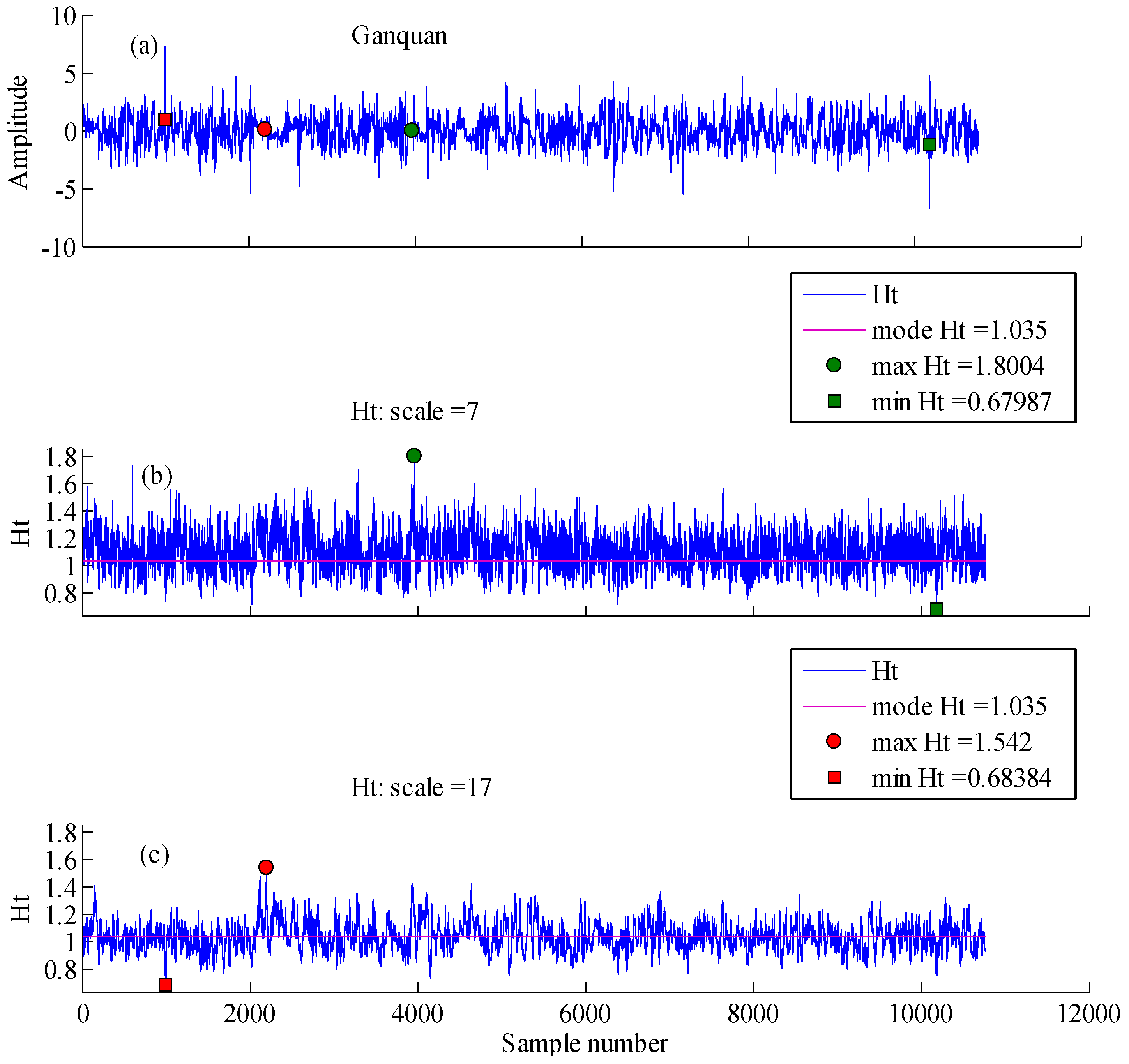
Loess ridge110°18′30′′–110°22′00′′ E; 37°33′00′′–36°35′00′′ NLocated in Ganquan, Shaanxi province, with an elevation between 990 and 1404 m, an average slope inclination of 27° and 7.74 km−1 of gully density. This area is characterized by an irregular bank-shaped distribution in morphology, which is almost a loess ridge with 200–300 m in width.
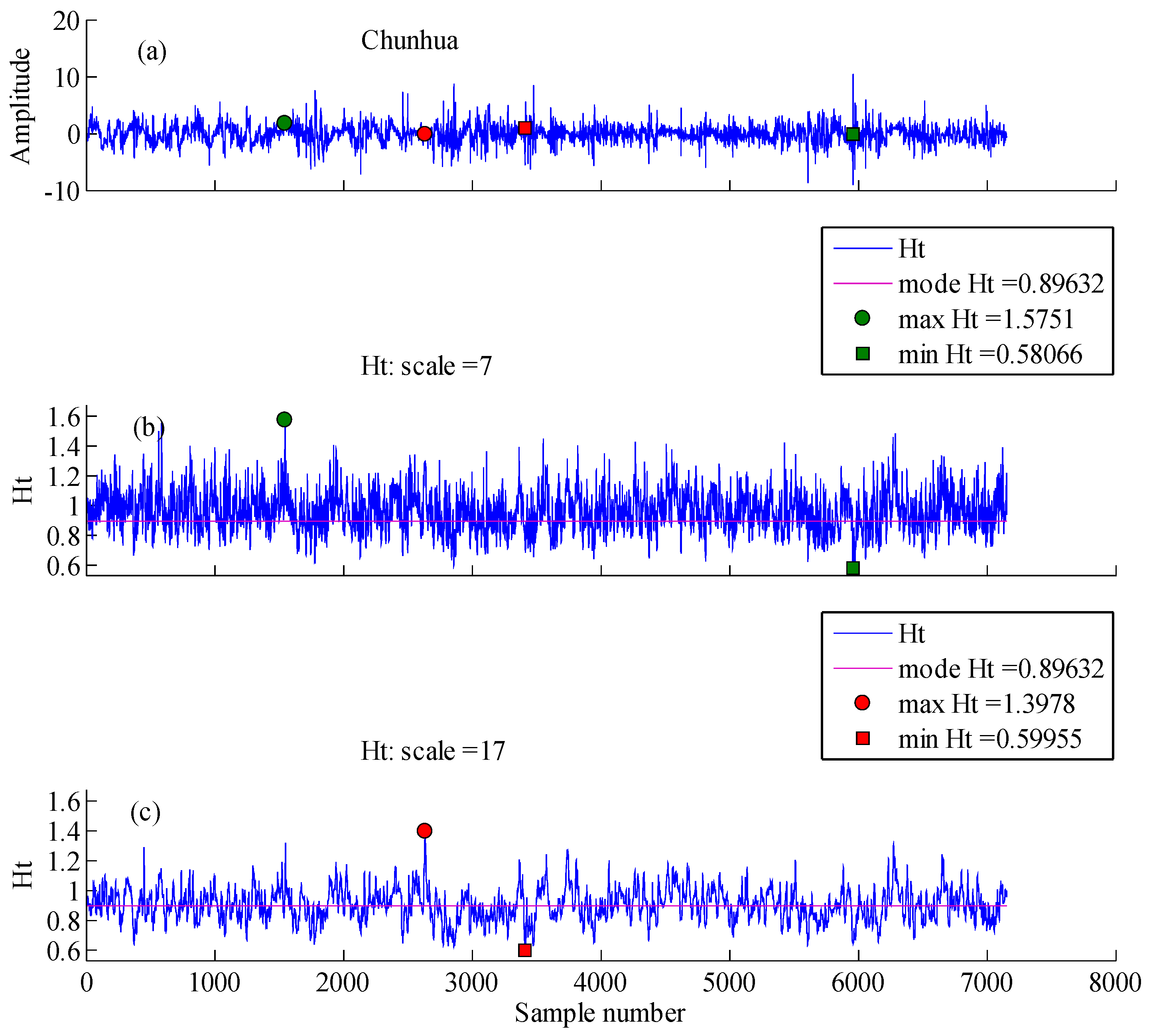
Loess tableland108°22′30′′–108°30′00′′ E; 34°50′00′′–34°55′00′′ NLocated in Chunhua, Shaanxi province, with an average elevation between 768 and 1188 m, an average slope inclination of 12, and 1.79 km−1 of gully density. The gentle slopes of land surface decreased the total soil loss by erosion.
Table 2. Parameters of multi-fractal analysis of the study sites.
SitesqtqhqDqHq Δ h q
Suide−5−5.86471.06450.54230.97290.6479
0−10.834410.8381
52.03480.41660.04820.6070
Ganquan−5−7.03911.38850.09651.20780.8945
0−10.868310.8755
52.18730.49400.28290.6375
Chunhua−5−6.35841.26070.05491.07170.6852
0−10.789010.7918
52.33430.57550.54310.6669

