
Upscaling of Surface Soil Moisture Using a Deep Learning Model with VIIRS RDR


School of Remote Sensing and Information Engineering, Wuhan University, Wuhan 430079, China
*
Author to whom correspondence should be addressed.
†
These authors contributed equally to the work.
ISPRS Int. J. Geo-Inf. 2017, 6(5), 130; https://doi.org/10.3390/ijgi6050130
Submission received: 7 March 2017
/
Revised: 19 April 2017
/
Accepted: 25 April 2017
/
Published: 27 April 2017
Abstract
:In current upscaling of in situ surface soil moisture practices, commonly used novel statistical or machine learning-based regression models combined with remote sensing data show some advantages in accurately capturing the satellite footprint scale of specific local or regional surface soil moisture. However, the performance of most models is largely determined by the size of the training data and the limited generalization ability to accomplish correlation extraction in regression models, which are unsuitable for larger scale practices. In this paper, a deep learning model was proposed to estimate soil moisture on a national scale. The deep learning model has the advantage of representing nonlinearities and modeling complex relationships from large-scale data. To illustrate the deep learning model for soil moisture estimation, the croplands of China were selected as the study area, and four years of Visible Infrared Imaging Radiometer Suite (VIIRS) raw data records (RDR) were used as input parameters, then the models were trained and soil moisture estimates were obtained. Results demonstrate that the estimated models captured the complex relationship between the remote sensing variables and in situ surface soil moisture with an adjusted coefficient of determination of = 0.9875 and a root mean square error (RMSE) of 0.0084 in China. These results were more accurate than the Soil Moisture Active Passive (SMAP) active radar soil moisture products and the Global Land data assimilation system (GLDAS) 0–10 cm depth soil moisture data. Our study suggests that deep learning model have potential for operational applications of upscaling in situ surface soil moisture data at the national scale.
1. Introduction
Soil moisture is a crucial variable in controlling the hydrologic cycle between the land surface and the atmosphere through vegetation evaporation and transpiration [1,2,3,4]. Accurate soil moisture estimation at a site is of great importance in modeling the surface hydrologic circle and climate change. Direct observations of ground measurements provide surface soil moisture with high accuracy and scalable frequency at the points measured. However, the most obvious limitations of the ground soil moisture measurements are their spatial discontinuity at specific locations [5], and, therefore, point-based or ground station measurements do not represent the spatial distribution since soil moisture varies spatiotemporally [6]. For the requirement of soil moisture estimation at a large scale (i.e., national scale), satellite remote sensing (RS) measurements are the preferred operational option. RS has shown great promise in providing improved spatial and temporal coverage of soil moisture measurements [7]. The main difficulties lie in how to accurately estimate the surface soil moisture. An effective method to enhance the accuracy of soil moisture estimates is to upscale in situ soil moisture measurements using RS measurements via statistical regression models. However, conventional statistical regression models have difficulties in extracting complex correlations between large-scale RS data and in situ soil moisture.
There are three types of upscaling methods. One type is land surface model based upscaling approach, which merges in situ soil moisture measurements with predictions of a land surface model. Cai et al. [8] used a hyper-resolution land surface model (HydroBlocks) to upscale in situ soil moisture measurements for the SMAP Validation Experiment 2015. Such models can accurately upscale in situ soil moisture measurements at the field-scale, depending on plenty of parameterizing ground data [9]. Therefore, the model-based method might not be suitable for large-scale applications of soil moisture upscaling with few ground-based parameters.
The second type uses traditional statistical regression methods to upscale in situ measurements with optical/IR RS indices or active/passive RS land surface parameters. Using polynomial regression statistics based on Universal Triangle methods Wang et al. [10,11] upscaled in situ soil moisture measurements using MODIS-based land surface temperature (LST) and normalized difference vegetation index (NDVI) data to map daily soil moisture products at 1 km resolution. By implementing a geostatistical algorithm, such as block kriging, researchers can compute the spatial semivariogram of surface soil moisture measurements at different stations in a local area and compute the surface soil moisture across the whole area [12,13]. Qin et al. [9,14] found that a Bayesian linear regression-based model performs better than the ordinary least square linear regression-based or the block kriging-based models when upscaling in situ soil moisture data with MODIS-based apparent thermal inertia (ATI) data. Based on the strategy of temporal stability and the high frequency of in situ soil moisture observations [15], stations with temporally continuous measurements have been selected to build a linear regression model based on in situ soil moisture data. However, the complexity and nonlinearity of the relationships makes it impossible to obtain large-scale estimates using traditional statistical regression methods.
The third type of approach involves using machine learning methods, such as support vector regression (SVR), and artificial neural networks (ANN). These methods can usually achieve more accurate soil moisture estimates than traditional statistical regression method because they can better model nonlinear relationships without special mathematic equations or assumptions about the data distribution based on larger-scale soil samples. Sajjad et al. [16] have found that an SVR-based model performed better than an ANN-based model when upscaling in situ soil moisture at 12 km resolution with resampled TRMM backscatter and resampled AVHRR NDVI data. However, constructing a stable regression relationship between these RS variables and in situ data remains challenging because it is difficult to extract the complicated nonlinearities from large training datasets. Recently, deep learning networks have been introduced to learn useful representations from large unlabeled datasets and has been applied for classification and regression in many fields [17,18]. When applied to a well-known benchmark, i.e., the recognition of handwritten digits in the Mixed National Institute of Standards and Technology database, the best reported error rates are 1.6% for shallow neural network using randomly initialized backpropagation and 1.4% for support vector machines (SVMs) [17]. Multicolumn deep convolutional neural networks (CNN) were the first to achieve a near-human performance, with the best reported error rate of 0.23% [19]. RS applications, such as land cover classification [20], feature selection [21], and climatology prediction [22], use deep learning networks, but the use of these methods in soil moisture estimation at the national scale using RS data remains untested. The purpose of the present study is to investigate the possibility of using a deep neural network for upscaling of soil moisture with large-scale datasets sampled from in situ soil moisture and RS measurements.
In this paper, we propose a deep learning method based on a deep feedforward neural network (DFNN) to upscale in situ surface soil moisture data for cropland in China using VIIRS raw data records (RDR). VIIRS RDR refers to the raw data from the satellite (Suomi National Polar-Orbiting Partnership spacecraft launched on 28 October 2011) transmitted to the earth, which can be calibrated to radiance radiance/reflectance and brightness temperatures with geolocation, namely VIIRS sensor data records (SDR) [23]. We can obtain real-time daily VIIRS RDR received by the meteorological satellite direct broadcasting service system in the Ministry of Water Resources of China since 2012. In addition, the Ministry of Water Resources of China has the unique advantage of 1997 soil moisture ground stations and 10-day observations. Based on abundant satellite remote sensing and ground measurements and the compelling advantages of the deep learning techniques, we upscaled soil moisture ground measurements using VIIRS RDR to achieve a national surface soil moisture product at 750 m resolution.
The remainder of this paper is organized into the following four sections. Section 2 describes the data and the study area. Then, we describe the deep learning models with the input parameters and building procedure in Section 3. Section 4 discusses the calibrated models and the adjustments in the model training parameters and assesses the results of the model validation and the residual charts, which are used to discuss the model variance. The paper concludes with a summary of our findings in Section 5.
2. Study Area and Data
2.1. Study Area
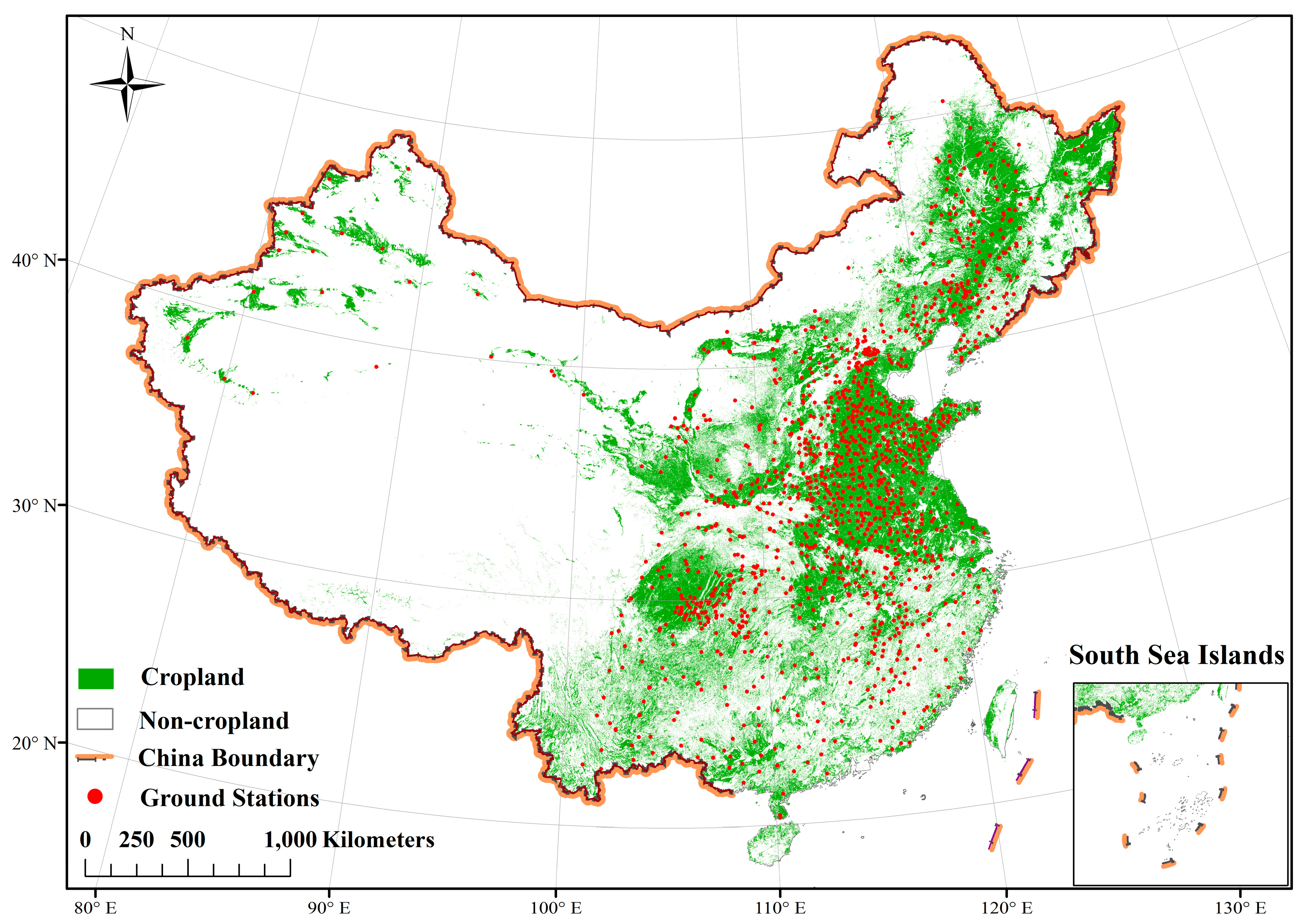
The focus of our study was China’s cropland, and these were delineated from GlobeLand30 [24,25] land use land cover (LULC) map produced in 2010. The data refers to 10 land cover types, namely cultivated land, forest, grassland, and others. We use cultivated land of GlobeLand30 as croplands masked from 2012 to 2015. The dataset can be found at the following link: http://www.globallandcover.com (last access date: 2 October 2016). The cropland mask was extracted by identifying cultivated land as one class and all nine other land cover types as a single non-cropland class. In Figure 1, the green regions denote cropland, and the white regions represent non-cropland areas.
2.2. Data
In addition to the GlobeLand30 2010 dataset, VIIRS SDR, in situ soil moisture measurements, precipitation ground observations, SMAP and GLDAS data were used in this study as follows.
(1) VIIRS RDR
VIIRS RDR has five imagery bands, sixteen moderate resolution bands and one day–night band, and, in this study, twelve moderate resolution bands were selected (See Table 1), where M1, M2, M3, M4, M5, M6, M7, M8, M10 and M11 were used to calculate the top of atmosphere (TOA) reflectance, and M12, M15 and M16 were used to calculate the TOA brightness temperature. These data were collected on the 1st, 11th, and 21st day of each month from May to October during each year from 2012 to 2015. M9, M13 and M14 were not chosen for this study because most of the band radiances would be absorbed by water vapor according to the atmospheric transmission profile [26].
(2) In situ soil moisture measurements
The croplands of China contain 1875 distributed ground stations for soil moisture observations (see the red points in Figure 1). The Chinese Ministry of Water Resources collects soil samples from all of the ground stations every 10 days to measure the soil moisture content in the top 10-cm soil layer by the gravimetric method [28]. In Figure 1, the red points represent the locations of the soil moisture sampling stations. The stations are sparse in western China and dense in the other regions. At these stations, soil samples were collected, and the soil moisture content of the upper 10-cm soil layer was measured gravimetrically [28]. We present the gravimetric soil moisture in percent in this article. These in situ soil moisture measurements were performed at 08:00 a.m. Beijing Time on the 1st, 11th, and 21st day of each month from May to October during each year from 2012 to 2015.
(3) Precipitation data
China Merged Precipitation Analysis (CMPA) with hourly, 0.1° × 0.1° resolution data [29] were collected to filter invalid soil moisture observations measured at the same date and time (06:00 a.m.–02:00 p.m.) as the in situ soil ground measurements.
(4) SMAP and GLDAS data
We compare the upscaling estimates over China cropland with the Soil Moisture Active Passive (SMAP) [30] active radar and Global Land data assimilation system (GLDAS) [31] soil moisture products to demonstrate the advantages of our model. SMAP is an orbiting observatory that measures the amount of water in the top 5 cm (2 inches) of soil everywhere on Earth’s surface, which is designed to measure soil moisture every 2–3 days over a three-year period. SMAP’s radar started transmitting data on January 2015, and it stopped on 7 July 2015 when its radar sensor broke. Therefore, only three months (May to July 2015) of SMAP radar daily soil moisture level 3 product (∼3 km resolution) corresponding to in situ soil moisture were obtained [30].
GLDAS produces global vertical layers (0–100 cm) of daily gravimetrical soil moisture (kg/cm2) every three hours at 25 km resolution [31]. Because the GLDAS soil moisture at 00:00 UTC matches the time of ground measurement, we use the upper layer (0–10 cm) of the GLDAS soil moisture at 00:00 every day at the same time range as SMAP for the research area. Readers can find these datasets by using the following link: https://search.earthdata.nasa.gov (last access date: 2 October 2016).
3. Methodology
3.1. Input Parameters of Soil Moisture Estimation Models
Short Wave Infrared (SWIR) reflectance of soil was proven to be sensitive to the surface soil moisture. Lobell and Anser [32] describe the relationship between the soil moisture and soil reflectance using the in situ soil moisture. For a given value of soil porosity, all of the bands of soil reflectance have a strong absorbing effect on soil moisture, especially in SWIR regions where the wavelength of soil reflectance band is approximately 1300 nm, 1900 nm and 2200 nm.
Corresponding to these regions, M7, M8, M10 and M11 are the four VIIRS solar reflectance bands (SRB). Those bands are defined as input parameters of MODEL I. Because visible/near infrared bands between 350 nm and 1000 nm are also correlated with surface soil moisture, they can also absorb surface soil moisture. M1, M2, M3, M4, M5, M6, M7, M8, M10 and M11 are used as input parameters of MODEL II. In addition, land surface temperature (LST) also has a linear relationship with surface soil moisture [33], which is the function of Thermal Emissive Bands (TEB). Therefore, M12, M15 and M16 are employed as input parameters of MODEL III.
- MODEL I:
- MODEL II:
- MODEL III:
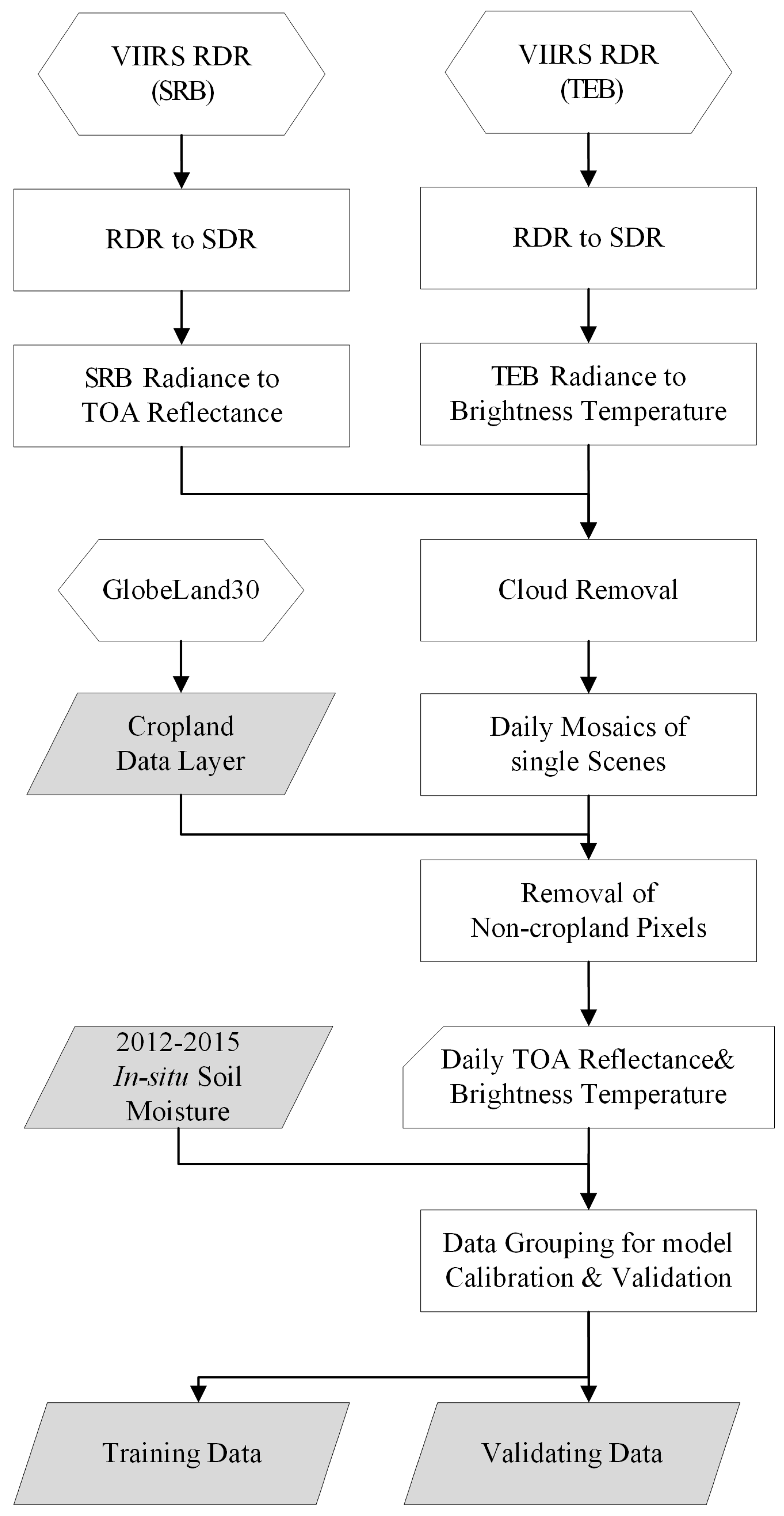
The model input calculation procedure includes the following steps (1)–(6), as shown in Figure 2.
(1) Convert VIIRS RDR to VIIRS SDR
Thirteen bands of VIIRS RDR are used in this study, including the raw data of ten SRB (M1, M2, M3, M4, M5, M6, M7, M8, M10, and M11) and three TEB (M12, M15 and M16). To convert RDR to the radiance of SRB and TEB, we used Community Satellite Processing Package (CSPP), SDR Version 2.2 Patch. Readers can find the package by using the following link: http://cimss.ssec.wisc.edu/cspp/npp_sdr_v2.2.3.shtml (last access date: 2 July 2016). This approach calculates the geolocation information and converts the data from raw counts to radiance.
(2) Convert SRB radiance and TEB radiance to TOA reflectance and brightness temperature, respectively.
To remove the Bow-tie effect at the edge of the single scene of VIIRS SDR, we performed geometric correction to derive the correct radiance using the geolocation file. In addition, the TOA reflectance was calculated by Equation (1), where L represents SRB radiance and EarthSun_dist denotes the distance between the earth and sun, which can be calculated using the current date. Band mean solar irradiance (BMSI) and solar zenith angle (SZA) are SRB constants which can be adapted from the header file of VIIRS SDR. The brightness temperature was calculated by Equation (2), where k denotes the Boltzmann constant, which is equal to ; h refers to Planck’s constant, which is equal to ; c represents the speed of light, which is equal to ; refers to wavelength of a certain VIIRS TEB; and L denotes to the pixel value of VIIRS TEB radiance.
(3) Cloud removal of single scenes of VIIRS image
To remove cloud, we employed the Fmask method [34] using both VIIRS TOA reflectance and brightness temperature since Fmask version 3.3 is proven to be an effective package for detecting cloud pixels in Landsat series, VIIRS SDR product and Sentinel 2 level 1 product efficiently and accurately [35].
(4) Daily mosaic of single scenes of TOA reflectance or brightness temperature
We mosaicked single scenes of TOA reflectance or brightness temperature with non-cloud pixels over the whole area of China. During the process, the pixel values of the overlapping regions were averaged for each pixel.
(5) Removal of non-cropland pixels
Since soil moisture is meaningful for sites at croplands in the research area, we removed non-cropland pixels such as water and urban areas. We used GlobeLand30 to exclude pixels with nine different land cover types differing from cropland.
(6) Data grouping for model calibration and validation
First, soil moisture measurements at 1875 ground stations were confined to the valid range of 0 to 100 and invalid measurements were screened out. Then, a total of 68,342 items of soil moisture measurements were kept by a no precipitation filter, ensuring the measuring time period of selected soil moisture measurements had no precipitation. In situ soil moisture measurements were linked with the calculated TOA reflectance or brightness temperature at the same location and time, which ensures that the three measurements were kept only if all of the data are valid. A total of 9789 pairs of samples were obtained by overlapping in situ soil measurements and TOA reflectance of VIIRS SWIR bands (M7, M8, M10, and M11); a total of 8096 pairs of samples were obtained by overlapping in situ soil measurements and TOA reflectance of VIIRS SWIR and Visible bands (M1, M2, M3, M4, M5, M6, M7, M8, M10, and M11); and a total of 6428 pairs of samples were obtained by overlapping in situ soil measurements and TOA reflectance of VIIRS SWIR and Visible bands (M1, M2, M3, M4, M5, M6, M7, M8, M10, M11, M12, M15, and M16). Finally, the valid soil samples were randomly split into model calibration (one-tenth of the samples) and validation datasets (nine-tenths of the samples). The datasets of each year (2012–2015) were split in the same way. The model calibration datasets were used as the input parameters of the deep learning model, while the model validation datasets were used to validate the calibrated models. The soil moisture estimation samples taken for training were independent of those taken for validation.
3.2. Model Building Using Deep Learning
Deep feedforward neural network (DFNN) was used because it is an established supervised tool that can produce a regression task to extract deep features among a large number of variables and enable high predictive accuracy. The H2O implementation of deep learning was used in this study, which is based on a DFNN that is trained with gradient descent using error back propagation. Readers can find the H2O R package 3.0 edition by using the following link: https://github.com/h2oai/h2o-3 (last access date: 22 December 2016).
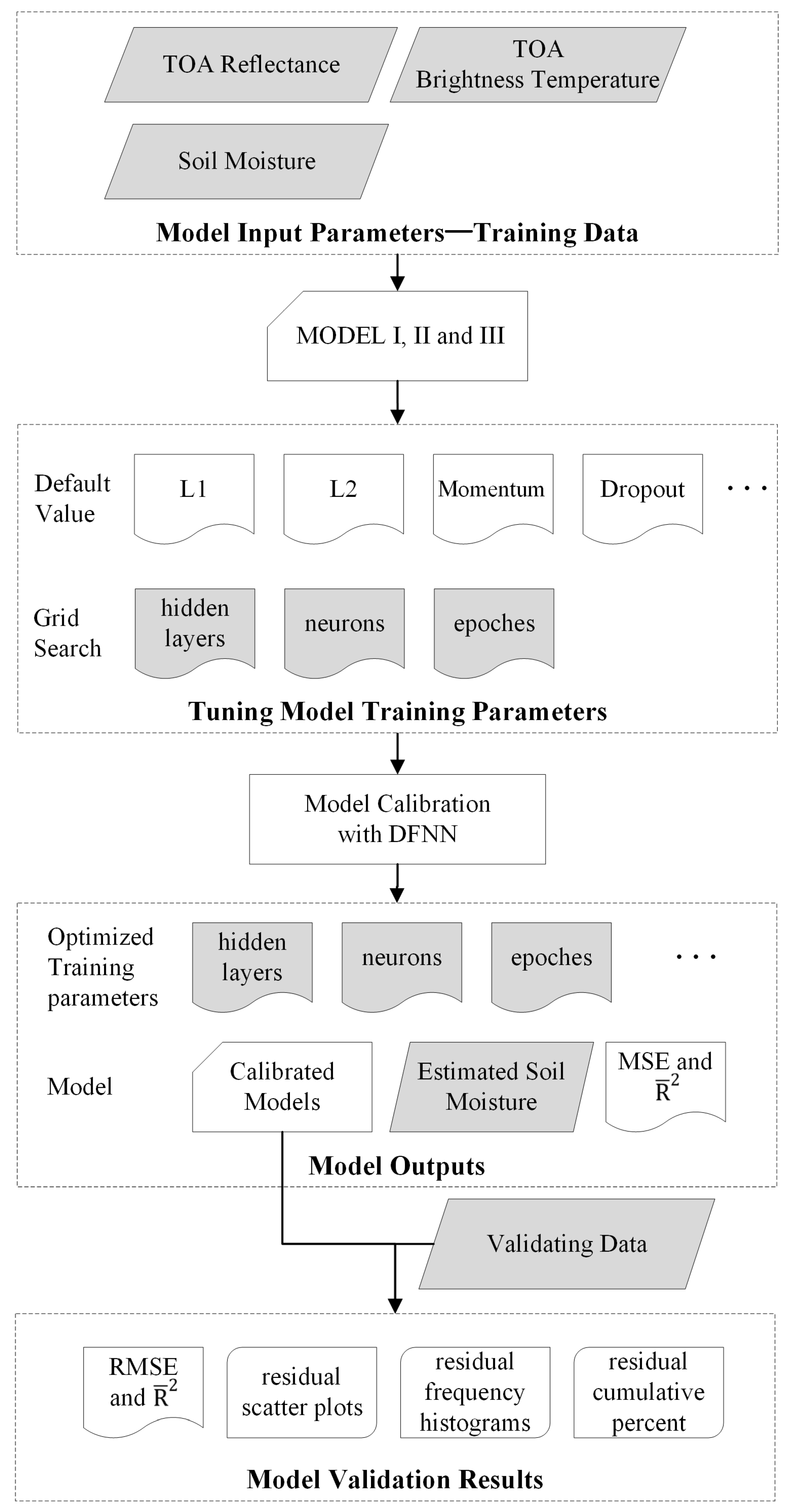
We built deep learning-based models including one input layer with two types of explanatory variables (VIIRS TOA reflectance and brightness temperature), one response variable (in situ soil moisture), one output layer (estimated soil moisture), and multiple hidden layers. The procedure of model building, as shown in Figure 3, includes the following steps.
(1) Tuning the model’s training parameters
The H2O deep learning model has more than 70 parameters [36]. To reduce the complexity of the H2O deep learning model, we adopted the recommended default values for the majority of model parameters, such as L1 = 0.2, L2 = 0.2, momentum_start = 0.5, input_dropout_ratio = 0.2, hidden_dropout_ratios = 0.5, and others, where L1, L2 and dropout are effective regularization techniques to prevent model overfitting. In addition, the default rectifier linear was used as the activation function. The H2O deep learning model enables the following constraining parameters: (1) the number of hidden layers; (2) the number of hidden units in each hidden layer, i.e., neurons; and (3) the number of iterations over the training samples, i.e., epochs. To address the optimal values, a grid search algorithm [37,38] was employed. For each model, the number of hidden layers started at 3 and ended at 11, neurons started at 100 and ended at 500, and epochs started at 1000 and ended at 3500. Then, after each iteration, the number of hidden layers, neurons and epochs would be increased by 1100 and 100, respectively. When the minimum MSE value and maximum are obtained, the optimal parameters are determined.
(2) Model calibration using DFNN
By tuning hidden layers, neurons and epochs, three groups of models can be calibrated when the highest and lowest MSE value occurs. The output of the calibration includes the calibrated models (model category, weights, biases, statues of neuron layers, etc.), the estimated soil moisture, and the optimized training parameters (hidden layers, neurons and epochs).
(3) Model validation using in situ soil moisture
The number of validating samples was approximately one tenth of total samples. All samples were independent of the training samples. To measure model variance and to further explore model performance, we performed residual analysis on estimated soil moisture and in situ soil moisture using residual scatter plots, residual frequency histograms, and residual cumulative percent plots. The residual scatter plots were employed to identify probable outliers under a conditional probability of 99.7%. Based on this confidence level, Jarque–Bera tests [39] were performed on the residual data to evaluate the normality of the models. Accompanied by residual frequency histograms and residual cumulative percent plots, the Jarque–Bera test uses the hypothesis that the data are normally distributed at the significance level of 0.3%. When the probability is lower than 0.003, the null hypothesis can be rejected and the data are normally distributed, and vice versa. Additionally, the Jarque–Bera test results can be used to determine whether the residual data have the skewness and kurtosis patterns that match those of a normal distribution.
4. Results and Discussion
4.1. Model Calibration Using DFNN
By tuning the number of hidden layers, neurons and epochs, we obtained and MSE for the three models, as shown in Table 2, Table 3 and Table 4, respectively. For Model I, we first used 10 hidden layers and 500 neurons. When the number of epochs was less than 1000, low value occurred; when the number of epochs was increased to 2000, the results had a significant agreement, with = 0.9746 and MSE = 0.0003. This finding demonstrates that a large number of epochs enables complex model learning pattern recognition and better prediction results in this situation. For nine hidden layers and 500 neurons, when the number of epochs was not equal to 1000, the results showed extreme instability and a poor correlation. When the number of epochs was equal to 3500, the results showed a significant agreement, with = 0.9786 and MSE = 0.0003. Hence, even relatively shallow layers led to good estimations. For Model II, we first used 10 hidden layers and 500 neurons. When the number of epochs was less than or equal to 1000, low value occurred; when the number of epochs was increased to 1300, the results had a significant goodness of fit, with = 0.9169 and MSE = 0.0005. For nine hidden layers and 400 neurons, when the number of epochs varied from 1000 to 1300, the results showed relatively poor correlation. For eight hidden layers, the results showed that a shallower layer DFNN can achieve better agreement of minimum MSE = 0.00009 and maximum = 0.9851, compared to relatively deeper layers in this situation. For Model III, when we used nine hidden layers and 400 neurons, the coefficients of determination of the model were relatively stronger than those when 10 hidden layers and 500 neurons were used. When the number of epochs was equal to 1300, the results showed a strong correlation, with = 0.9215 and MSE = 0.0005. For 8 hidden layers and 500 neurons, the result reached the highest goodness of fit, with minimum MSE = 0.00009 and maximum = 0.9851 when the number of epochs was equal to 3500.
4.2. Model Validation Using In Situ soil Moisture
The optimal versions of Model I (highlighted in Table 2) were validated using 1000 pairs of validation samples. As shown in Figure 4, the adjusted coefficients of determination were greater than 0.95, demonstrating that Model I was able to capture more than 95% of variability in measured soil moisture data. The model using 10 hidden layers was more stable compared to that using nine hidden layers for RMSE was reduced from 0.0282 to 0.0131. The optimal versions of Model II (highlighted in Table 3) were validated using 700 pairs of validation samples. The validation results were > 0.89 and RMSE < 0.03. While the adjusted coefficients of determination of the model validation results were lower than those of the model calibration results, one possible reason is that the relatively small sample size may have resulted in more instability for DFNN in the model calibration process. The optimal versions of Model III (highlighted in Table 4) were validated using 500 pairs of samples. Similar to Models I and II, the results demonstrated Model III could explain most of variability in measured soil moisture.
The models using eight hidden layers generated better results than those using more hidden layers. By comparing the three groups of models, we observed that deep neural hidden layers are not suitable for relatively small-scale datasets containing 5900 to 7300 samples. At the same time, the iterative operations in the model training of Model II and III were more computationally intensive than that of Model I. This is mainly because Models II and III have higher dimensions of input parameters than Model I. In addition, using Model III is better if the size of the training data are relatively small due to the multi-sensor remote sensing data. In contrast, we suggest using Model I to estimate soil moisture when the size of soil samples is relatively large with only visible remote sensing data.
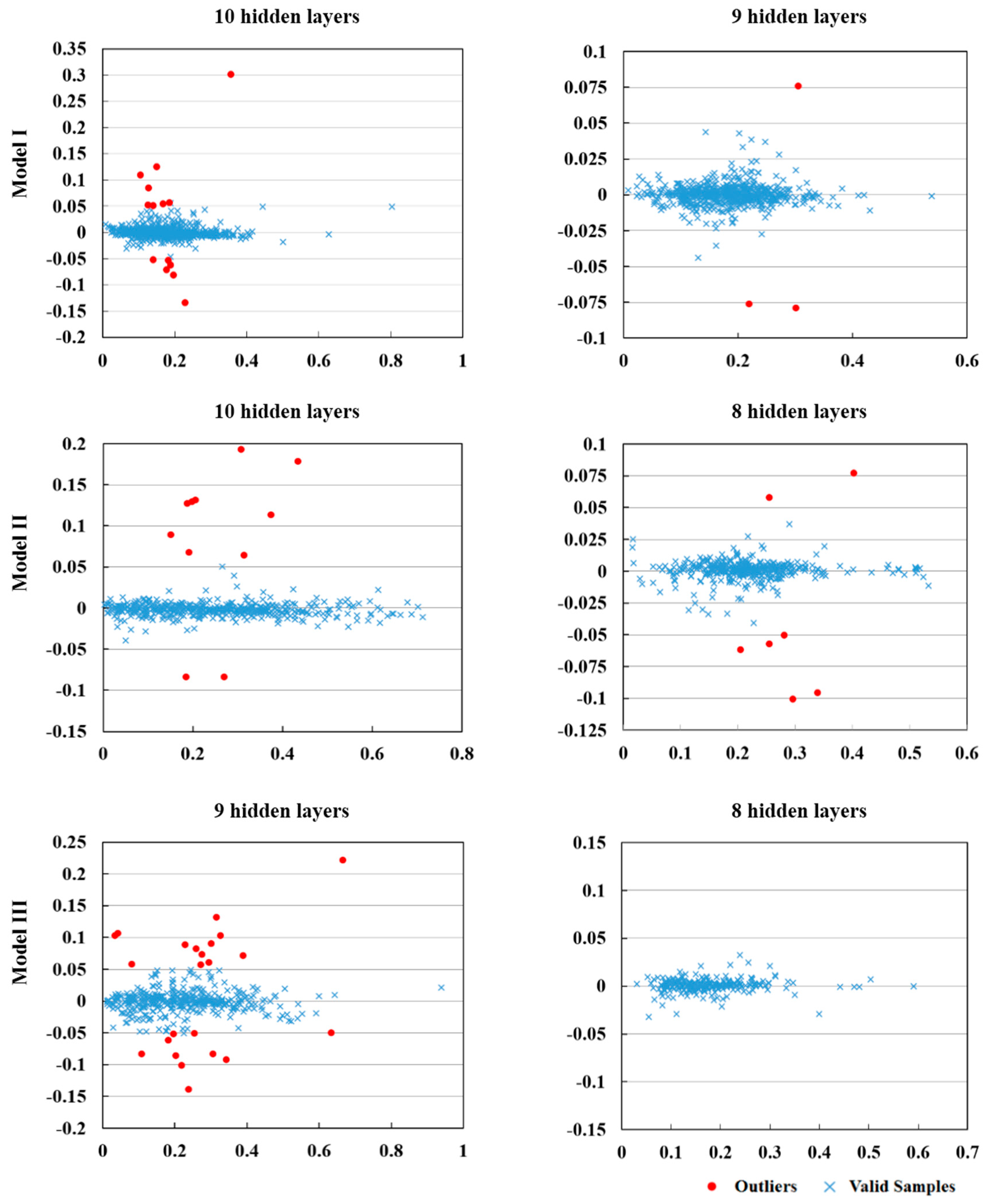
4.3. Residual Analysis
Figure 5 shows the residual scatter plots of the models, the x-axis represents the in situ soil moisture value of samples and y-axis represents the residual value between model estimated and in situ measured soil moisture. The red points were probable outliers that were identified using confidence intervals with a conditional probability of 99.7%. Based on this confidence level, the Jarque–Bera test was performed on the residual data to evaluate the normality of the models.
As shown in Figure 6, statistical significance of each model is less than 0.003, and the skewness is close to 0. This result demonstrates that the residual data of all models obeyed normal distribution. Specifically, for the optimal versions of Model I, the kurtosis of the model using 10 hidden layers is larger than that of the model using nine hidden layers, while the skewness of two models is opposite. The results indicated that the models with more hidden layers have greater statistical significance and more stable performance compared to those with less hidden layers for Model I. This conclusion was further confirmed by the probable outliers shown in Figure 5, and the number of probable outliers of the model using 10 hidden layers was greater than that of the model using nine hidden layers. The same conclusion can be drawn for the optimal versions of Model III. Conversely, for the optimal versions of Model II, the kurtosis of the model using eight hidden layers is larger than that of the model using 10 hidden layers, while the skewness of the two models is opposite to the kurtosis. One possible reason is that the large number of epochs (3500) could have resulted in overlearning problems and instability in the network’s generalization capability [40].
4.4. Comparison with SMAP and GLDAS Soil Moisture Product
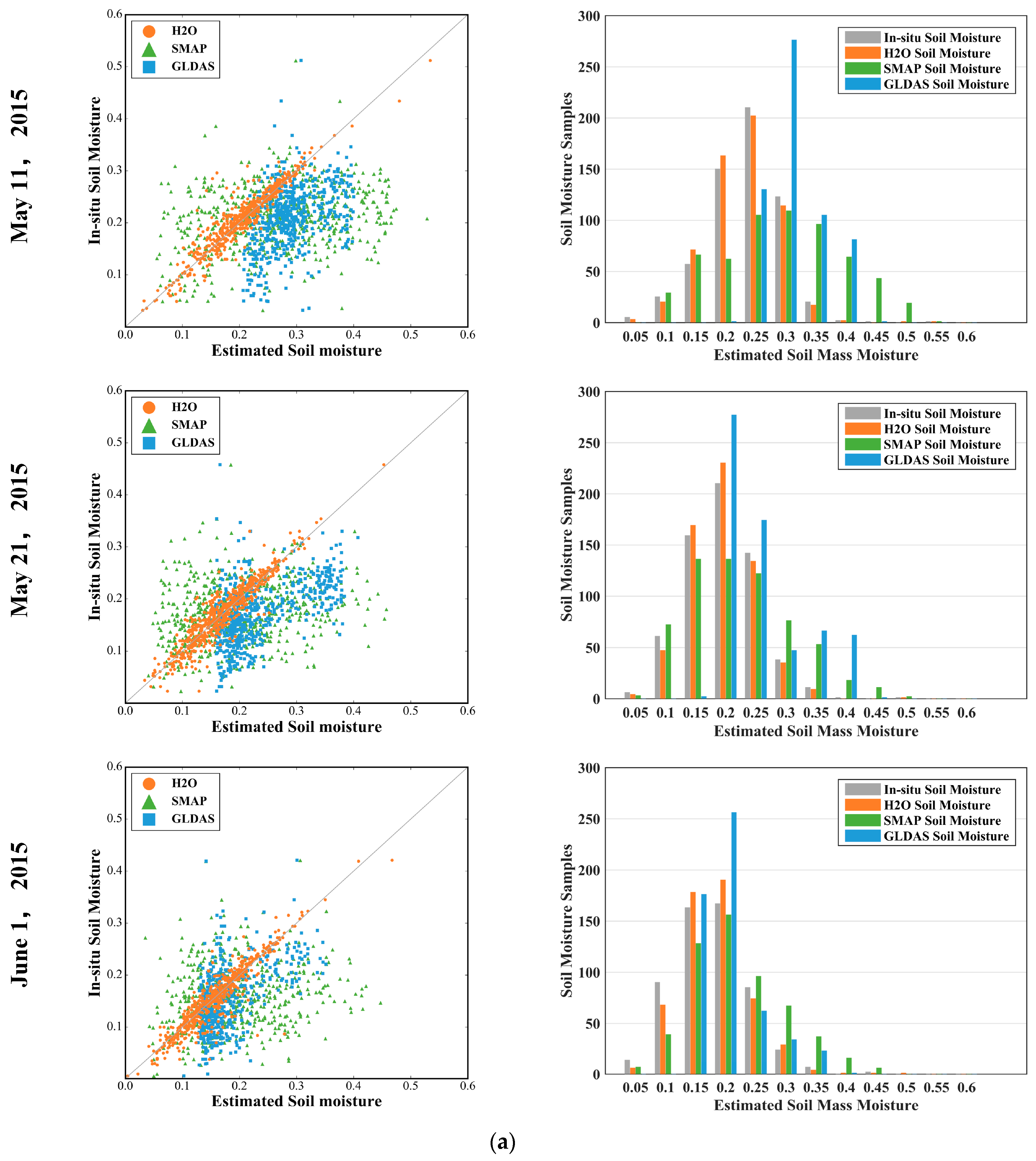
To further investigate the performance of the H2O model estimates, we employed the soil moisture product of SMAP and GLDAS to compare with the upscaling results estimated by MODEL III (8 hidden layers). Based on the dates of the in situ soil moisture measurements, we selected the three types of soil moisture estimates on six individual days (11 May 2015, 21 May 2015, 1 June 2015, 11 June 2015, 21 June 2015 and 1 July 2015). The 2–3-day revisit period causes large data gaps in the SMAP daily soil moisture product. Therefore, we mosaicked three SMAP soil moisture images for each revisit period to represent the six days. In detail, images on 10–12 May were mosaicked to represent 11 May; 19–21 May were mosaicked to represent 21 May; 30 and 31 May and 1 June were mosaicked to represent 1 June 2015; 10–12 June were mosaicked to represent 11 June; 19–21 June were mosaicked to represent 21 June; and 29 and 30 June and 1 July were mosaicked to represent 1 July. We obtained 594, 629, 552, 605, 584, and 553 pairs of soil samples, respectively, for the six single days, and each pair includes the H2O model-based soil moisture estimate, SMAP radar-based soil moisture estimate, GLDAS soil moisture estimate and in situ soil moisture for the same day and location. Then, we used , RMSE and p-value to validate three types of soil moisture estimates against in situ soil moisture measurements, as shown in Figure 7 and Table 5.
In Figure 7, where the panels on the left show the 1:1 scatter plots of three types of soil moisture estimates compared to in situ soil moisture measurements. The panels on the right are the corresponding distribution histograms of the soil samples on the six days. The H2O models performed better for soil moisture estimation than SMAP radar product and GLDAS product. The distribution pattern of their soil samples displayed the same trend. At the same time, the majority of the SMAP soil moisture values have a range of 0.15–0.25, indicating a systematic over-estimation problem compared to the in situ soil moisture measurements. One possible reason is that the measurement unit of the SMAP soil moisture is cm3/cm3 (water volume divided by water and soil volume), which differs from that of in situ soil moisture, i.e., g/g (water weight divided by water and soil weight). Theoretically, the volume water percentage is equal to the result of the gravimetric soil moisture multiplied by the density of water and soil. Strictly speaking, the density of the water and soil is greater than 1; as a result, the majority of the SMAP soil moisture results are greater than the in situ soil moisture measurements. For GLDAS, the points plot closer to the 1:1 line than those of the SMAP but farther than those of H2O, in accordance with the correlation results shown in Table 5.
The H2O model fitted the in situ soil moisture best at the 0.05 level (p < 0.05) and estimated soil moisture most accurately (RMSE is minimal) among the three types of soil moisture products. For GLDAS, the scaling effect created a more serious spatial mismatch problem: the point-based ground soil sample cannot represent all of the land cover in a GLDAS soil moisture pixel. The GLDAS soil moisture product has a resolution of 25 km and is far coarser than the VIIRS resolution of 750 m and the SMAP radar resolution of 3 km. In addition, the GLDAS soil moisture product averages the soil moisture values from 00:00 to 03:00 UTC due to a 3-h lag with respect to the ground measuring time (00:00 UTC). This difference could lead to uncertainty and error in the soil moisture estimation due to possible evapotranspiration by corn or irrigation occurring during the lag period. Similarly, a larger time difference between the SMAP overpass (06:00 UTC) and the in situ soil moisture could lead to greater uncertainty and error in soil moisture estimation compared to GLDAS.
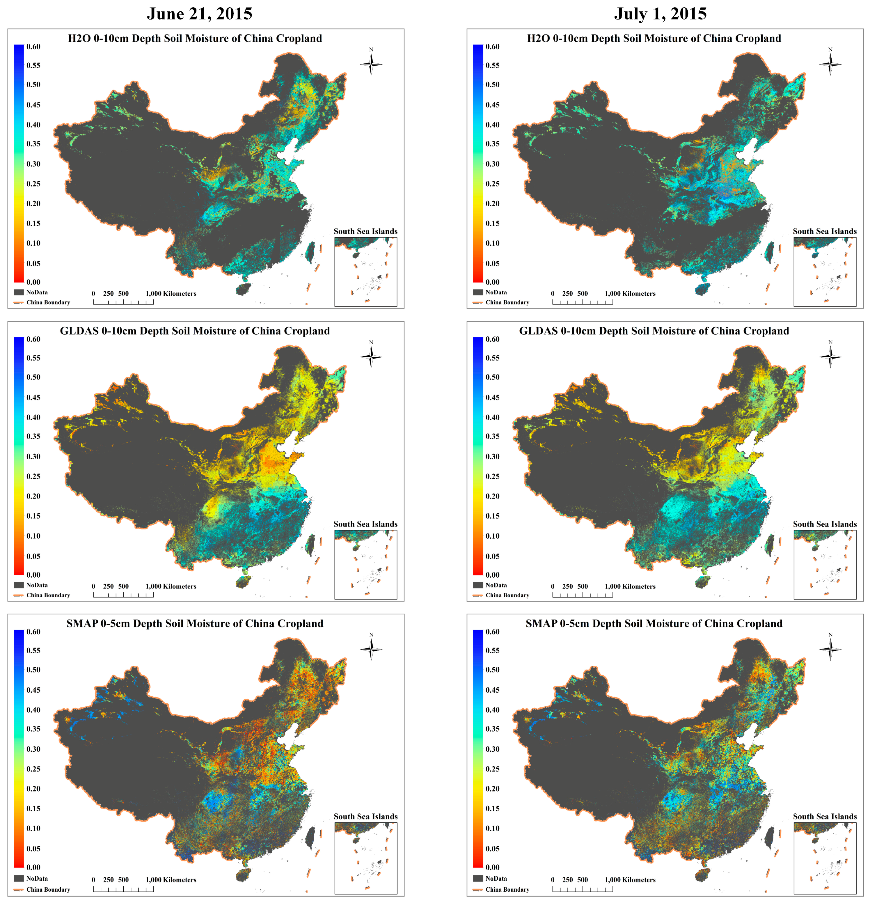
The SMAP radar appears to be worse at capturing the variance in ground measured soil moisture than GLDAS. This is mainly due to the different value ranges between SMAP volumetric soil moisture and in situ measured gravimetric soil moisture. In addition, SMAP radar-based soil moisture estimates are less accurate (RMSE is the maximal) than GLDAS soil moisture estimates. This may have caused by two factors, one is the low signal-to-noise ratio of SAMP radar due to radio frequency interference [41,42]. The other is that SMAP can only measuring the top 5 cm depth of soil surface layer without sampling 0–100 cm in depth like GLDAS. The H2O model-based soil moisture estimation maps have a resolution of 750 m and are finer than the GLDAS resolution of 25 km and the SMAP radar resolution of 3 km. As Figure 8 shows, H2O model based soil moisture estimates represent more details spatially than other two products. Nonetheless, it is not perfect, due to a missing data problem associated with cloud removal.
5. Conclusions
This paper proposed a deep learning model-based method for upscaling in situ soil moisture using VIIRS RDR to address the challenging problem of surface soil moisture estimation at the national scale. Three groups of models were built using VIIRS SWIR, Visible/SWIR, and Visible/SWIR/TIR data. The results showed high accuracy with 0.8917 < < 0.9813 and 0.0118 < RMSE < 0.0294, thereby confirming the effectiveness of the deep learning model. The results also showed that models using eight hidden layers should be employed when the size of the training samples is relatively small and the dimension of the input variables is relatively large (multi-sensor). For the upscaling of the in situ soil moisture to the national scale, we suggest using a model with eight hidden layers, 500 neurons per hidden layer, and 3500 epochs per hidden layer. We observed that the effectiveness of these models depended on the model parameters and the size of the input training dataset. To make the models more operational, further work is necessary. Our approach produces surface soil moisture estimated for cropland in China that are more accurate than the SMAP radar soil moisture products and GLDAS 0–10 cm depth soil moisture products. However, the soil moisture map has data gaps due to clouds in image data. Still, the deep learning models provided a practical way to upscale the soil moisture to a national scale. We believe that they can be applied more comprehensively when more remote sensing sensors such as radar are involved.
Acknowledgments
We gratefully acknowledge the funding support for this research provided by the National High-Resolution Earth Observation System Projects (civil part): Hydrological monitoring system by high spatial resolution remote sensing image (first phase) (08-Y30B07-9001-13/15).
Author Contributions
Dongying Zhang designed the experiment and procedure. Wen Zhang analyzed the results and together they wrote the manuscript. The work was supervised by Lingkui Meng, who contributed to all stages of the work. Wei Huang made major contributions to the interpretations and modification. Zhiming Hong performed the model validation experiment.
Conflicts of Interest
The authors declare no conflict of interest.
References
- Chen, F.; Mitchell, K.; Schaake, J.; Xue, Y.; Pan, H.L.; Koren, V.; Duan, Q.Y.; Ek, M.; Betts, A. Modeling of land surface evaporation by four schemes and comparison with fife observations. J. Geophys. Res. Atmos. 1996, 101, 7251–7268. [Google Scholar] [CrossRef]
- Wang, L.; Qu, J.J. Satellite remote sensing applications for surface soil moisture monitoring: A review. Front. Earth Sci. China 2009, 3, 237–247. [Google Scholar] [CrossRef]
- Lakshmi, V. Remote sensing of soil moisture. ISRN Soil Sci. 2013, 2013. [Google Scholar] [CrossRef]
- Fang, B.; Lakshmi, V. Soil moisture at watershed scale: Remote sensing techniques. J. Hydrol. 2014, 516, 258–272. [Google Scholar] [CrossRef]
- Petropoulos, G.P. Remote Sensing of Energy Fluxes and Soil Moisture Content; CRC Press: Boca Raton, FL, USA, 2013. [Google Scholar]
- Engman, E.T. Applications of microwave remote sensing of soil moisture for water resources and agriculture. Remote Sens. Environ. 1991, 35, 213–226. [Google Scholar] [CrossRef]
- Wagner, W.; Naeimi, V.; Scipal, K.; de Jeu, R.; Martínez-Fernández, J. Soil moisture from operational meteorological satellites. Hydrogeol. J. 2007, 15, 121–131. [Google Scholar] [CrossRef]
- Cai, X.; Pan, M.; Chaney, N.W.; Colliander, A.; Misra, S.; Cosh, M.H.; Crow, W.T.; Jackson, T.J.; Wood, E.F. Validation of smap soil moisture for the smapvex15 field campaign using a hyper-resolution model. Water Resour. Res. 2017. [Google Scholar] [CrossRef]
- Qin, J.; Zhao, L.; Chen, Y.; Yang, K.; Yang, Y.; Chen, Z.; Lu, H. Inter-comparison of spatial upscaling methods for evaluation of satellite-based soil moisture. J. Hydrol. 2015, 523, 170–178. [Google Scholar] [CrossRef]
- Carlson, T. An overview of the “triangle method” for estimating surface evapotranspiration and soil moisture from satellite imagery. Sensors 2007, 7, 1612–1629. [Google Scholar] [CrossRef]
- Wang, L.; Qu, J.; Zhang, S.; Hao, X.; Dasgupta, S. Soil moisture estimation using modis and ground measurements in eastern china. Int. J. Remote Sens. 2007, 28, 1413–1418. [Google Scholar] [CrossRef]
- Vinnikov, K.Y.; Robock, A.; Qiu, S.; Entin, J.K. Optimal design of surface networks for observation of soil moisture. J. Geophys. Res. 1999, 1041, 19743–19750. [Google Scholar] [CrossRef]
- Wang, J.; Ge, Y.; Song, Y.; Li, X. A geostatistical approach to upscale soil moisture with unequal precision observations. IEEE Geosci. Remote Sens. Lett. 2014, 11, 2125–2129. [Google Scholar] [CrossRef]
- Qin, J.; Yang, K.; Lu, N.; Chen, Y.; Zhao, L.; Han, M. Spatial upscaling of in-situ soil moisture measurements based on modis-derived apparent thermal inertia. Remote Sens. Environ. 2013, 138, 1–9. [Google Scholar] [CrossRef]
- De Rosnay, P.; Gruhier, C.; Timouk, F.; Baup, F.; Mougin, E.; Hiernaux, P.; Kergoat, L.; LeDantec, V. Multi-scale soil moisture measurements at the gourma meso-scale site in mali. J. Hydrol. 2009, 375, 241–252. [Google Scholar] [CrossRef]
- Ahmad, S.; Kalra, A.; Stephen, H. Estimating soil moisture using remote sensing data: A machine learning approach. Adv. Water Resour. 2010, 33, 69–80. [Google Scholar] [CrossRef]
- Hinton, G.E.; Salakhutdinov, R.R. Reducing the dimensionality of data with neural networks. Science 2006, 313, 504–507. [Google Scholar] [CrossRef] [PubMed]
- Salakhutdinov, R.; Hinton, G. Semantic hashing. Int. J. Approx. Reason. 2009, 50, 969–978. [Google Scholar] [CrossRef]
- Ciresan, D.; Meier, U.; Schmidhuber, J. Multi-column deep neural networks for image classification. In Proceedings of the 2012 IEEE Conference on Computer Vision and Pattern Recognition (CVPR), IEEE, Washington, DC, USA, 16–21 June 2012; pp. 3642–3649. [Google Scholar]
- Chen, Y.; Lin, Z.; Zhao, X.; Wang, G.; Gu, Y. Deep learning-based classification of hyperspectral data. IEEE J. Sel. Top. Appl. Earth Obs. Remote Sens. 2014, 7, 2094–2107. [Google Scholar] [CrossRef]
- Zou, Q.; Ni, L.; Zhang, T.; Wang, Q. Deep learning based feature selection for remote sensing scene classification. IEEE Geosci. Remote Sens. Lett. 2015, 12, 2321–2325. [Google Scholar] [CrossRef]
- Kühnlein, M.; Appelhans, T.; Thies, B.; Nauss, T. Improving the accuracy of rainfall rates from optical satellite sensors with machine learning—A random forests-based approach applied to msg seviri. Remote Sens. Environ. 2014, 141, 129–143. [Google Scholar] [CrossRef]
- Cao, C.; Xiong, X.; Wolfe, R.; DeLuccia, F.; Liu, Q.; Blonski, S.; Lin, G.; Nishihama, M.; Pogorzala, D.; Oudrari, H. Visible Infrared Imaging Radiometer Suite (Viirs) Sensor Data Record (sdr) User’s Guide; Version 1.2; NOAA Technical Report NESDIS: Washington, DC, USA, 2013; Volume 142, p. 15.
- Jun, C.; Ban, Y.; Li, S. China: Open access to earth land-cover map. Nature 2014, 514, 434. [Google Scholar] [CrossRef] [PubMed]
- Chen, J.; Chen, J.; Liao, A.; Cao, X.; Chen, L.; Chen, X.; He, C.; Han, G.; Peng, S.; Lu, M. Global land cover mapping at 30 m resolution: A pok-based operational approach. ISPRS J. Photogramm. Remote Sens. 2015, 103, 7–27. [Google Scholar] [CrossRef]
- Li, Z.; Tan, D. The second modified perpendicular drought index (mpdi1): A combined drought monitoring method with soil moisture and vegetation index. J. Indian Soc. Remote Sens. 2013, 41, 873–881. [Google Scholar] [CrossRef]
- Xiong, X.; Butler, J.J.; Chiang, K.; Efremova, B.; Fulbright, J.P.; Lei, N.; Mcintire, J.; Oudrari, H.; Sun, J.; Wang, Z. Viirs on-orbit calibration methodology and performance. J. Geophys. Res. 2014, 119, 5065–5078. [Google Scholar] [CrossRef]
- China’s Ministry of Water Resources (MWR). Technical Standard for Soil Moisture Monitoring; China Water Power Press: Beijing, China, 2015.
- Shen, Y.; Zhao, P.; Pan, Y.; Yu, J. A high spatiotemporal gauge-satellite merged precipitation analysis over china. J. Geophys. Res. Atmos. 2014, 119, 3063–3075. [Google Scholar] [CrossRef]
- Entekhabi, D.; Njoku, E.G.; Neill, P.E.; Kellogg, K.H.; Crow, W.T.; Edelstein, W.N.; Entin, J.K.; Goodman, S.D.; Jackson, T.J.; Johnson, J. The soil moisture active passive (smap) mission. Proc. IEEE 2010, 98, 704–716. [Google Scholar] [CrossRef]
- Rui, H.; Beaudoing, H. Readme Document for Global Land Data Assimilation System Version 2 (Gldas-2) Products; GES DISC: Greenbelt, MD, USA, 2011.
- Lobell, D.B.; Asner, G.P. Moisture effects on soil reflectance. Soil Sci. Soc. Am. J. 2002, 66, 722–727. [Google Scholar] [CrossRef]
- Lakshmi, V.; Jackson, T.J.; Zehrfuhs, D. Soil moisture–temperature relationships: Results from two field experiments. Hydrol. Process. 2003, 17, 3041–3057. [Google Scholar] [CrossRef]
- Zhu, Z.; Woodcock, C.E. Object-based cloud and cloud shadow detection in landsat imagery. Remote Sens. Environ. 2012, 118, 83–94. [Google Scholar] [CrossRef]
- Zhu, Z.; Wang, S.; Woodcock, C.E. Improvement and expansion of the fmask algorithm: Cloud, cloud shadow, and snow detection for landsats 4–7, 8, and sentinel 2 images. Remote Sens. Environ. 2015, 159, 269–277. [Google Scholar] [CrossRef]
- Candel, A.; Parmar, V.; LeDell, E.; Arora, A. Deep Learning with H2O; H2O. ai Inc.: Mountain View, CA, USA, 2016. [Google Scholar]
- Bengio, Y.; Courville, A.C.; Vincent, P. Representation learning: A review and new perspectives. IEEE Trans. Pattern Analys. Mach. Intell. 2013, 35, 1798–1828. [Google Scholar] [CrossRef] [PubMed]
- Larochelle, H.; Erhan, D.; Courville, A.; Bergstra, J.; Bengio, Y. An empirical evaluation of deep architectures on problems with many factors of variation. In Proceedings of the 24th International Conference on Machine Learning, Corvallis, OR, USA, 20–24 June 2007; ACM: New York, NY, USA; pp. 473–480. [Google Scholar]
- Jarque, C.M.; Bera, A.K. A test for normality of observations and regression residuals. Int. Stat. Rev. 1987, 55, 163–172. [Google Scholar] [CrossRef]
- Erhan, D.; Manzagol, P.-A.; Bengio, Y.; Bengio, S.; Vincent, P. The difficulty of training deep architectures and the effect of unsupervised pre-training. In Proceedings of the International Conference on Artificial Intelligence and Statistics, Clearwater Beach, FL, USA, 16–18 April 2009; pp. 153–160. [Google Scholar]
- Wagner, W.; Lemoine, G.; Rott, H. A method for estimating soil moisture from ers scatterometer and soil data. Remote Sens. Environ. 1999, 70, 191–207. [Google Scholar] [CrossRef]
- Pan, M.; Cai, X.; Chaney, N.W.; Entekhabi, D.; Wood, E.F. An initial assessment of smap soil moisture retrievals using high-resolution model simulations and in situ observations. Geophys. Res. Lett. 2016, 43, 9662–9668. [Google Scholar] [CrossRef]
Figure 1.
Ground stations for cropland soil moisture measurements in China.

Figure 2.
The procedure of the model input calculation.

Figure 3.
The procedure of model building.

Figure 4.
Comparison between in situ soil moisture and estimated soil moisture as obtained by the optimal versions of Model I, Model II and Model III.
Figure 4.
Comparison between in situ soil moisture and estimated soil moisture as obtained by the optimal versions of Model I, Model II and Model III.
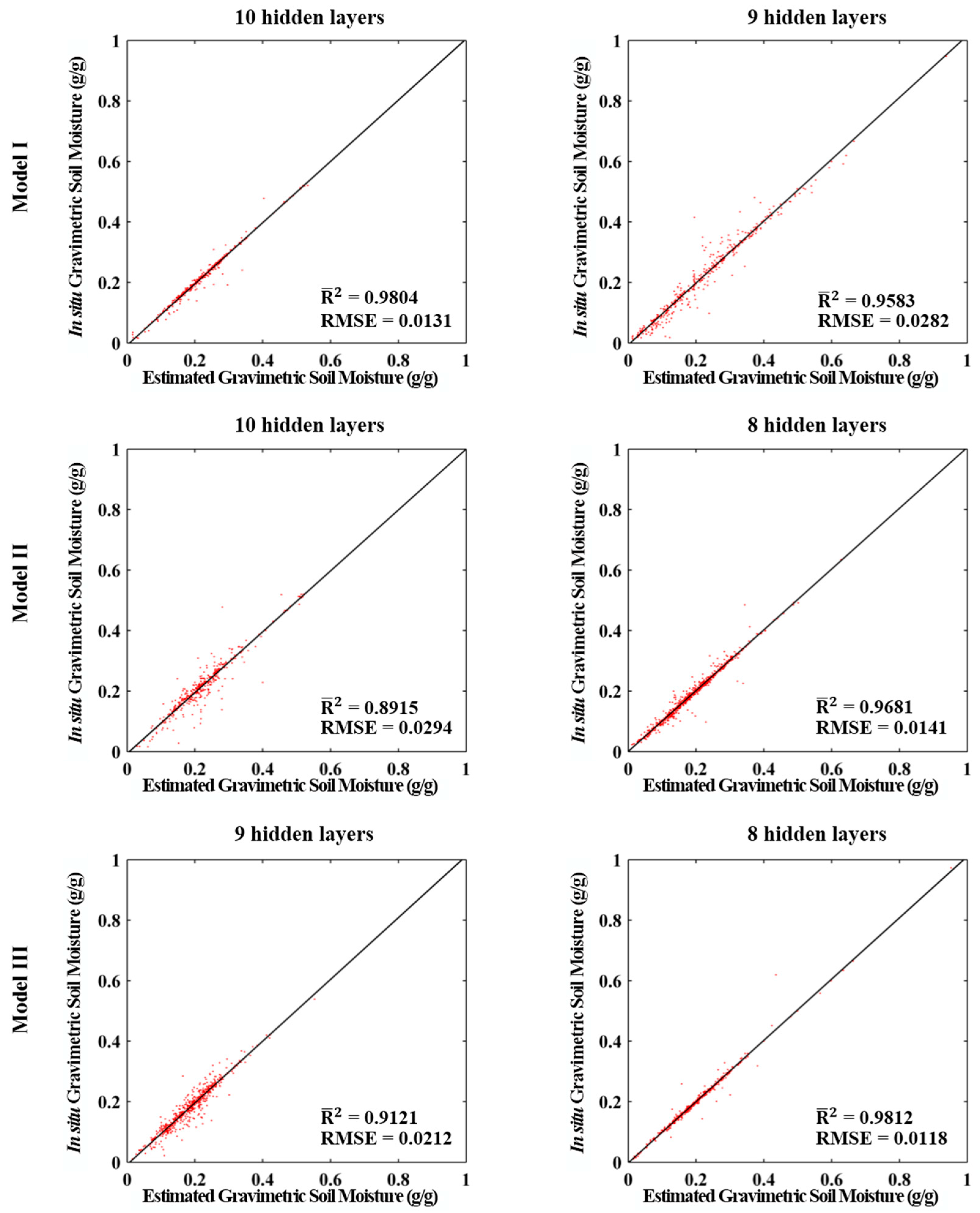
Figure 5.
The residual scatter plots of the three groups of optimal models.

Figure 6.
The residual frequency histograms and residual cumulative percent plots of three groups of optimal models.
Figure 6.
The residual frequency histograms and residual cumulative percent plots of three groups of optimal models.
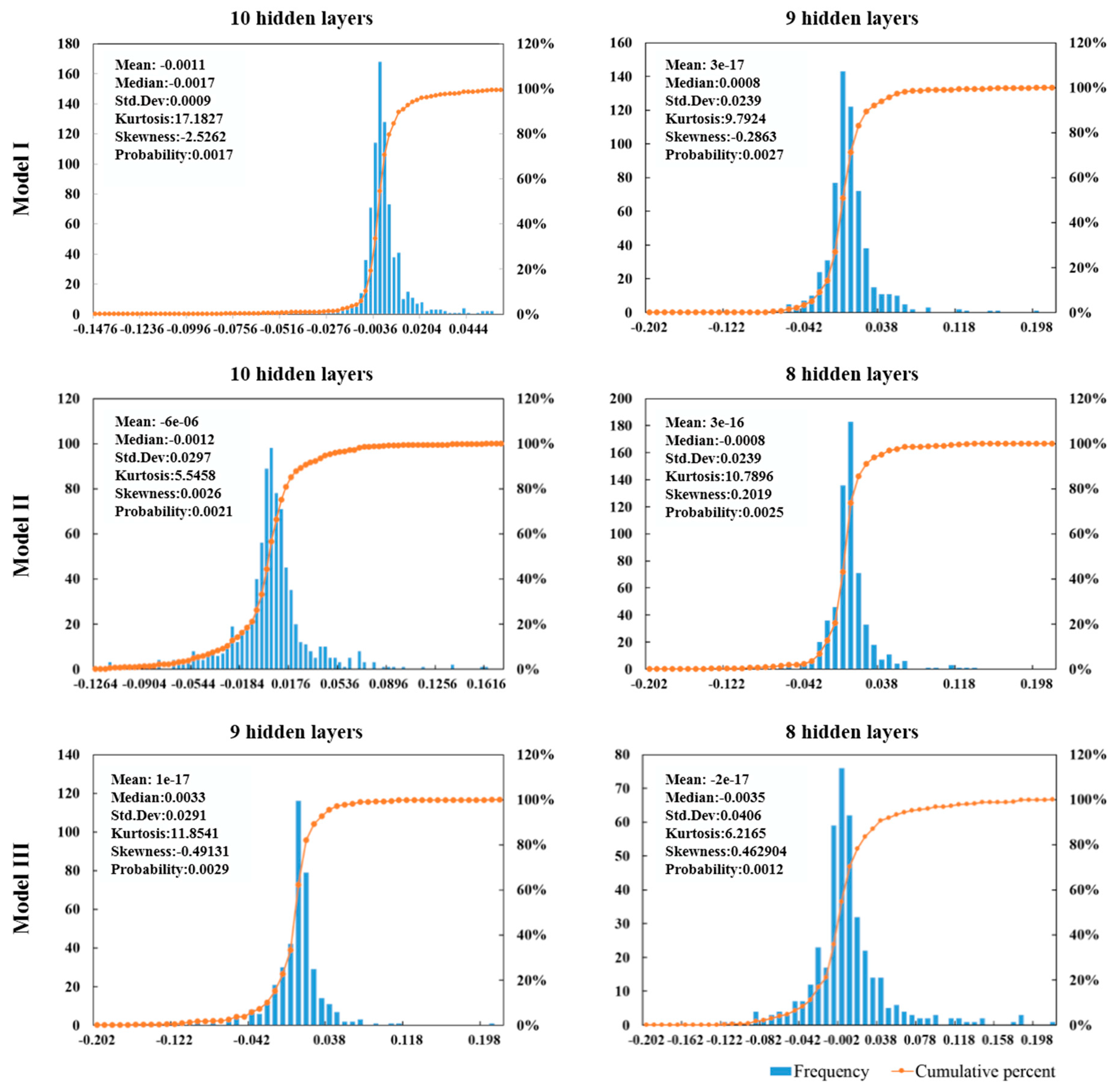
Figure 7.
(a) Comparison of the performance of three types of soil moisture estimates and in situ soil moisture measurements on 11 May, 21 May and 1 June 2015. (b) Comparison of the performance of three types of soil moisture estimates and in situ soil moisture measurements on 11 June, 21 June and 1 July 2015.

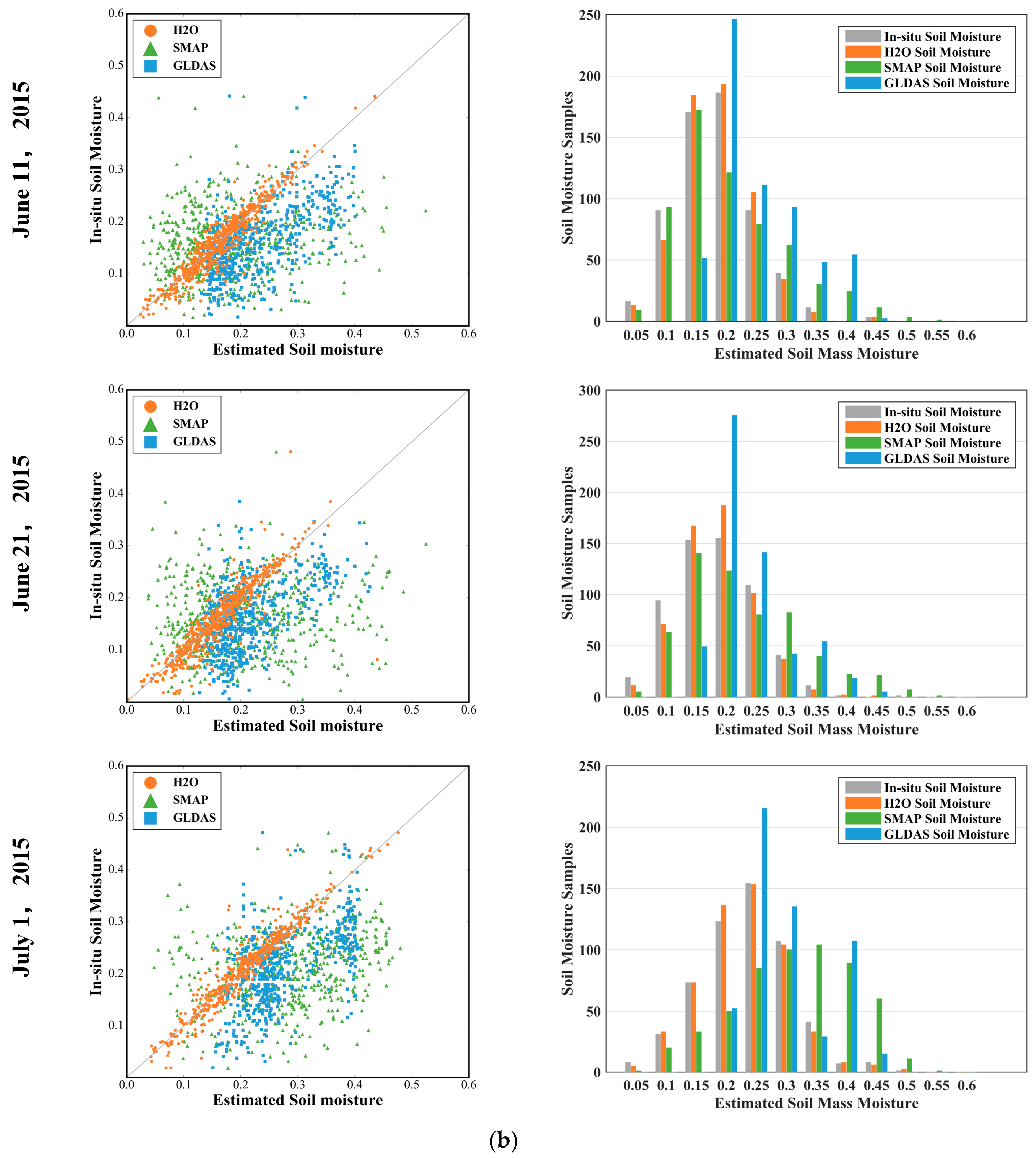
Figure 8.
H2O model estimated soil moisture at 0–10 cm depth, SMAP radar estimated soil moisture at 0–5 cm depth and GLDAS estimated soil moisture at 0–10 cm depth maps for cropland in China on 21 June and 1 July 2015.
Figure 8.
H2O model estimated soil moisture at 0–10 cm depth, SMAP radar estimated soil moisture at 0–5 cm depth and GLDAS estimated soil moisture at 0–10 cm depth maps for cropland in China on 21 June and 1 July 2015.


Table 1.
Specification of sixteen moderate resolution bands of Visible Infrared Imaging Radiometer Suite (VIIRS) raw data records (RDR) [27].
Table 1.
Specification of sixteen moderate resolution bands of Visible Infrared Imaging Radiometer Suite (VIIRS) raw data records (RDR) [27].
| Band Number (VIIRS) | Central Wavelength (nm) | Wavelength Range (nm) | Signal to Noise Ratio (SNR) or Noise Equivalent Differential Temperature (NEdT) (18 March 2013) |
|---|---|---|---|
| M1 | 412 | 402–422 | 1.72 |
| M2 | 445 | 436–454 | 1.56 |
| M3 | 488 | 478–498 | 1.54 |
| M4 | 555 | 545–565 | 1.50 |
| M5 | 672 | 662–682 | 1.30 |
| M6 | 746 | 739–754 | 1.69 |
| M7 | 865 | 846–885 | 1.80 |
| M8 | 1240 | 1230–1250 | 2.60 |
| M9 | 1378 | 1371–1386 | 2.47 |
| M10 | 1610 | 1580–1640 | 1.60 |
| M11 | 2250 | 2230–2280 | 2.14 |
| M12 | 3700 | 3610–3790 | 0.30 |
| M13 | 4050 | 3970–4130 | 0.37 |
| M14 | 8550 | 8400–8700 | 0.66 |
| M15 | 10763 | 10,260–11,260 | 0.43 |
| M16 | 12013 | 11,540–12,490 | 0.42 |
Table 2.
Parameters and Results of Model I.
| Hidden Layers | Neurons | Epochs | Samples | Time (s) | MSE | |
|---|---|---|---|---|---|---|
| 11 | 500 | 1000 | 8789 | 2922 | 0.3564 | 0.0107 |
| 11 | 300 | 1000 | 8789 | 4828 | 0.7543 | 0.0066 |
| 10 | 500 | 2000 | 8789 | 4995 | 0.9746 | 0.0003 |
| 10 | 500 | 1500 | 8789 | 7956 | 0.9301 | 0.0007 |
| 10 | 500 | 1000 | 8789 | 6771 | 0.8601 | 0.0008 |
| 9 | 500 | 3500 | 8789 | 3318 | 0.9786 | 0.0002 |
| 9 | 500 | 1500 | 8789 | 2895 | 0.8565 | 0.0008 |
| 9 | 300 | 1000 | 8789 | 2321 | 0.7115 | 0.0015 |
| 8 | 500 | 3500 | 8789 | 1250 | 0.3141 | 0.0453 |
Table 3.
Parameters and Results of Model II.
| Hidden Layers | Neurons | Epochs | Samples | Time (s) | MSE | |
|---|---|---|---|---|---|---|
| 10 | 500 | 1300 | 7396 | 3645 | 0.9169 | 0.0005 |
| 10 | 500 | 1200 | 7396 | 2874 | 0.8778 | 0.0008 |
| 10 | 500 | 1000 | 7396 | 2571 | 0.7334 | 0.0011 |
| 9 | 400 | 1300 | 7396 | 3016 | 0.6142 | 0.0065 |
| 9 | 400 | 1200 | 7396 | 2268 | 0.8303 | 0.0011 |
| 9 | 400 | 1000 | 7396 | 1728 | 0.7492 | 0.0016 |
| 8 | 500 | 3600 | 7396 | 3350 | 0.5141 | 0.0153 |
| 8 | 500 | 3500 | 7396 | 3032 | 0.9851 | 0.00009 |
| 8 | 500 | 3000 | 7396 | 2921 | 0.7115 | 0.0015 |
Table 4.
Parameters and Results of Model III.
| Hidden Layers | Neurons | Epochs | Samples | Time (s) | MSE | |
|---|---|---|---|---|---|---|
| 10 | 500 | 1200 | 5928 | 2426 | 0.6232 | 0.0019 |
| 10 | 500 | 1100 | 5928 | 2295 | 0.8365 | 0.0008 |
| 10 | 500 | 1000 | 5928 | 1828 | 0.6764 | 0.0026 |
| 9 | 400 | 1500 | 5928 | 1421 | 0.8115 | 0.0006 |
| 9 | 400 | 1300 | 5928 | 1287 | 0.9215 | 0.0005 |
| 9 | 400 | 1000 | 5928 | 977 | 0.8601 | 0.0008 |
| 8 | 500 | 3600 | 5928 | 3392 | 0.7142 | 0.0051 |
| 8 | 500 | 3500 | 5928 | 3250 | 0.9875 | 0.00007 |
| 8 | 500 | 3000 | 5928 | 2921 | 0.8036 | 0.0007 |
Table 5.
Comparison of the performance of three types of soil moisture estimates.
| Samples | p-Value | RMSE (%) | ||
|---|---|---|---|---|
| 11 May 2015 | ||||
| H2O | 594 | 0.8798 | <0.05 | 0.0213 |
| GLDAS | 594 | 0.1638 | <0.05 | 0.0975 |
| SMAP | 594 | 0.0609 | <0.05 | 0.1174 |
| 21 May 2015 | ||||
| H2O | 629 | 0.8671 | <0.05 | 0.0211 |
| GLDAS | 629 | 0.2950 | <0.05 | 0.0840 |
| SMAP | 629 | 0.0491 | <0.05 | 0.0940 |
| 1 June 2015 | ||||
| H2O | 552 | 0.8578 | <0.05 | 0.0228 |
| GLDAS | 552 | 0.2524 | <0.05 | 0.0595 |
| SMAP | 552 | 0.0370 | <0.05 | 0.0959 |
| 11 June 2015 | ||||
| H2O | 605 | 0.9080 | <0.05 | 0.0198 |
| GLDAS | 605 | 0.3518 | <0.05 | 0.0891 |
| SMAP | 605 | 0.0333 | <0.05 | 0.1029 |
| 21 June 2015 | ||||
| H2O | 584 | 0.8233 | <0.05 | 0.0281 |
| GLDAS | 584 | 0.2726 | <0.05 | 0.0811 |
| SMAP | 584 | 0.0078 | <0.05 | 0.1186 |
| 1 July 2015 | ||||
| H2O | 553 | 0.9193 | <0.05 | 0.0217 |
| GLDAS | 553 | 0.3298 | <0.05 | 0.0900 |
| SMAP | 553 | 0.0784 | <0.05 | 0.1274 |
© 2017 by the authors. Licensee MDPI, Basel, Switzerland. This article is an open access article distributed under the terms and conditions of the Creative Commons Attribution (CC BY) license (http://creativecommons.org/licenses/by/4.0/).
Share and Cite
MDPI and ACS Style
Zhang, D.; Zhang, W.; Huang, W.; Hong, Z.; Meng, L. Upscaling of Surface Soil Moisture Using a Deep Learning Model with VIIRS RDR. ISPRS Int. J. Geo-Inf. 2017, 6, 130. https://doi.org/10.3390/ijgi6050130
AMA Style
Zhang D, Zhang W, Huang W, Hong Z, Meng L. Upscaling of Surface Soil Moisture Using a Deep Learning Model with VIIRS RDR. ISPRS International Journal of Geo-Information. 2017; 6(5):130. https://doi.org/10.3390/ijgi6050130
Chicago/Turabian StyleZhang, Dongying, Wen Zhang, Wei Huang, Zhiming Hong, and Lingkui Meng. 2017. "Upscaling of Surface Soil Moisture Using a Deep Learning Model with VIIRS RDR" ISPRS International Journal of Geo-Information 6, no. 5: 130. https://doi.org/10.3390/ijgi6050130
Note that from the first issue of 2016, this journal uses article numbers instead of page numbers. See further details here.