Development of a Change Detection Method with Low-Performance Point Cloud Data for Updating Three-Dimensional Road Maps

Department of Civil Engineering, The University of Tokyo, 7-3-1 Hongo Bunkyo, Tokyo 113-8656, Japan
*
Author to whom correspondence should be addressed.
ISPRS Int. J. Geo-Inf. 2017, 6(12), 398; https://doi.org/10.3390/ijgi6120398
Submission received: 24 October 2017
/
Revised: 17 November 2017
/
Accepted: 1 December 2017
/
Published: 4 December 2017
(This article belongs to the Special Issue Mapping for Autonomous Vehicles)
Abstract
:Three-dimensional (3D) road maps have garnered significant attention recently because of applications such as autonomous driving. For 3D road maps to remain accurate and up-to-date, an appropriate updating method is crucial. However, there are currently no updating methods with both satisfactorily high frequency and accuracy. An effective strategy would be to frequently acquire point clouds from regular vehicles, and then take detailed measurements only where necessary. However, there are three challenges when using data from regular vehicles. First, the accuracy and density of the points are comparatively low. Second, the measurement ranges vary for different measurements. Third, tentative changes such as pedestrians must be discriminated from real changes. The method proposed in this paper consists of registration and change detection methods. We first prepare the synthetic data obtained from regular vehicles using mobile mapping system data as a base reference. We then apply our proposed change detection method, in which the occupancy grid method is integrated with Dempster–Shafer theory to deal with occlusions and tentative changes. The results show that the proposed method can detect road environment changes, and it is easy to find changed parts through visualization. The work contributes towards sustainable updates and applications of 3D road maps.
1. Introduction
1.1. Research Background
The applications of three-dimensional (3D) road maps have garnered significant attention in recent times. These maps express the geometrical shapes and structures in street environments as 3D objects. So far, most road maps are two-dimensional maps, and are used for navigation and road management. Recent developments in measurement technology, such as mobile mapping systems (MMS), can be used for transforming these two-dimensional maps into three-dimensional maps. An MMS is equipped with cameras and LASER (Light Amplification by Stimulated Emission of Radiation) scanners, and can easily and efficiently acquire 3D data on the street. 3D road maps are expected to facilitate applications in many fields. These maps will not only enhance driver navigation and road management, but also serve as base maps in disaster prevention and infrastructure management. The development of 3D maps is also keenly discussed in the field of autonomous driving because accurate and information-rich maps are needed for recognition, decision and operation, in order to replace the functions of human drivers. It is therefore appropriate that road maps for autonomous driving must contain information on dynamic and real-time street states, such as traffic accidents and road constructions [1]. Road maps expressing the street environment with 3D objects are important as base maps, and are being widely researched and discussed.
While MMS is generally considered an established means for constructing 3D road maps, people have now begun to discuss the maintenance of these maps. Map updating is important because 3D road maps contain much larger amounts of information than ordinary two-dimensional maps, and need to provide up-to-date information on the street environment for safety, especially in autonomous driving. The direct approach for keeping the map up to date is to build the road map repeatedly. In other words, the whole street area is measured by MMS and the map is rebuilt. This approach has the advantage of high accuracy, but is expensive, and obtaining point cloud data from MMS requires manual processes. Thus, the direct approach is prohibitive, and an alternative method is needed. A cost-saving alternative is to use the image or point cloud data from cheap sensors that regular vehicles are equipped with for supporting drivers and autonomous driving. It will be common in the near future for regular vehicles to have LASER scanners to scan the environment, when driver supporting systems or autonomous driving technology will be widespread. Thus, we would be able to easily obtain low cost point cloud data of the street environment if the data from regular vehicles is used. However, the data obtained from cheap sensors is not as accurate as that of MMS, and the updated map becomes a patchwork of data of varying accuracies.
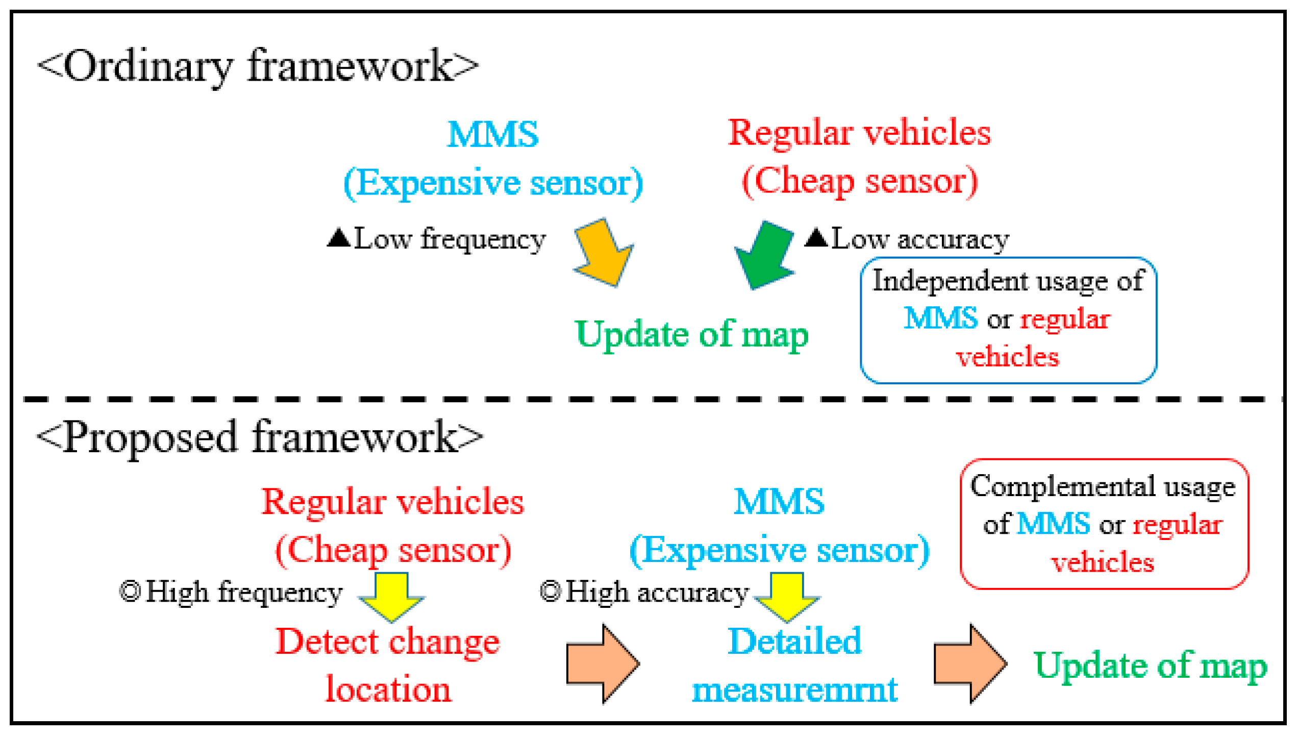
As discussed above, a method to update three-dimensional maps that satisfactorily addresses both frequency and accuracy requirements has not yet been established, and a framework that combines the best of both these approaches is needed. We propose a two-step approach (Figure 1). The changed locations are first detected using data from cheap sensors, and then detailed measurement is subsequently taken in those areas by using MMS. It will be possible to efficiently detect where changes in the road environment happen because data from regular vehicles can be frequently acquired, and the accuracy of the updated map would be consistent because MMS is used to acquire data for the map update. Thus, the proposed framework will contribute towards the sustainable updating of 3D road maps.
The research in this paper focuses on the first step, and visualizes the location of change in the street to enable us to quickly and easily understand where changes in the road environment occur. We deal with point cloud data in this paper because it is robust against climate and light conditions unlike image data. Moreover, point cloud data directly provides 3D information, while additional processing is required to obtain this information from image data. Nevertheless, there are several technical challenges that need to be addressed in order to achieve the proposed objective. Firstly, data from MMS and cheap sensors have different accuracies and point densities. The cheap sensors would also vary between themselves in terms of performance. Secondly, the measurement ranges of cheap sensors are likely to vary. Thirdly, the data would contain tentative changes, such as oncoming vehicles and pedestrians, which must be discriminated from real changes. We first align the low accuracy data with MMS data to adjust for position and rotation errors. We then apply the occupancy grid method [2] for change detection, because this method is robust to varying densities in the point cloud. In addition, we use Dempster–Shafer theory [3,4] to discriminate between occlusions and real changes in the occupancy grid method. Finally, only real changes are detected based on occupancy rate transitions.
1.2. Related Work
This section largely describes related work in two areas, registration and change detection. Many of the prior studies in these areas have been independently developed. Registration is the process of superimposing acquired data on the model data by applying rotation and translation transformations. Generally, the process of registration is divided into course registration and fine registration. Course registration provides initial values for the process of fine registration. Before course registration, the detection and description of feature points are carried out. Thus, the first half of this section describes previous research on the detection and description of feature points, course and fine registration. Following that, change detection methods are introduced for both image and point cloud-based data.
Detection of feature points is generally done as a preparation for registration. Feature points are defined as points expressing geometrical features of objects such as edges and peaks. There are a variety of ways of extracting feature points. Some methods have developed as applications of methods in image processing. For example, 3DSIFT [5] is an application of SIFT (Scale Invariant Feature Transform) [6] for point cloud data. Similarly, 3DHarris [7] is also an application of an image processing method. Guo et al. [8] provide a review of research that compares these detection methods.
After feature points in multiple point cloud data are detected, they are associated, and their description is carried out. Association methods are mainly divided into two categories. Methods of the first category describe the relationship between a point of interest and its neighbors, and those of the second category focus on relationships between pairs of interesting points [9]. In the first category, the Spin Image method and its derivations are widely used [10]. Some methods use normal vectors as descriptors of feature points, such as Point Feature Histogram (PFH) [11], Fast Point Feature Histogram (FPFH) [12], derivations of PFH on calculating cost, and Signature of Histogram of OrienTations (SHOT) [13]. In the second category, the Point Pair Feature (PPF) method picks a pair of points, and uses the distance and the angle of the normal vector as feature values [14]. The first category is known to be robust against noise, and the second is robust against occlusion. In addition to these, methods that use not only geometrical features but also color information have been developed, such as Color-SHOT [15] and PFHRGB [16]. Prior research has shown that using feature points reduces calculation costs, but does not always improve registration results [17]. Moreover, it is reported that the performance of descriptors depends on the shape of the objects [18].
Course registration methods can be classified into two types [19]. Methods of the first type associate points based on feature values calculated at several points. In this category, the methods that extract features such as spin image or principal component analysis are used to detect overlapping parts between data of interest. Methods of the second type work with matching points. The greedy initial alignment method and the SAmple Consensus Initial Alignment (SAC-IA) method are used together with PFH and FPFH, respectively. Course registration provides initial values for fine registration. There has been much research on fine registration, but the Iterative Closest Point (ICP) algorithm is the most classic and well-known example [20]. At about the same period when the ICP algorithm was developed, similar research using depth images was done [21]. There are several research publications on the selection of point pairs in the ICP algorithm. In a previous study [22], random sampling points are set as feature points, and similarly, in another method, the feature points are randomly selected in each registration [23]. For these methods, the normal space sampling method is introduced to make them more efficient and robust to noise [24].
Other than a few exceptions [25], most of the change detection methods only use image or point cloud data. In this study, we only work with point cloud data. To detect changes between two point clouds, a basic method is to look for differences based on the distance between points. If the distances between pairs of points are larger than a threshold, then this area is considered to have changed. However, this approach is not robust against noise or differences in point density. The Hausdorff distance is known to be robust against data damages [26].
The distance-based approach also has the disadvantage that it does not distinguish between occlusions and real changes because the distance between corresponding points tends to be larger in that area. Thus, some research has tried to distinguish real change from occlusion. Some research has used the occupancy method with Dempster–Shafer theory to deal with this problem, and have applied point cloud data from ALS (Airborne Laser Scanning) in two periods [27,28], and data from MMS [29,30]. The occupancy grid method was developed in robotics to build an environment map for an autonomous moving robot. The updating of the map is based on Bayes’ theory in many cases [31]. On the other hand, the introduction of Dempster–Shafer theory allows us to consider occlusion explicitly. However, because frameworks using Bayes’ theory require lower calculation costs than those using Dempster–Shafer theory, the latter approach has not been used much, while its advantages have nevertheless been confirmed [32,33].
While previous studies using the occupancy grid method with Dempster–Shafer theory have had the advantage of being able to distinguish real changes from occlusions, another problem remains. They have been able to successfully reject occlusions, but the results contain tentative changes of oncoming vehicles and pedestrians. Due to this, they cannot be directly applied for updating the map. Methods for the detection of moving objects have been separately developed, mainly in the image processing fields [34]. Recently, integrated methods for both images and point clouds have appeared [35,36], but the detection of changes and moving objects are yet to be integrated.
Based on the above summary of related work, the challenges are summarized as follows:
- Distinguishing real changes from occlusions and tentative changes,
- Detecting changes in point cloud data with varying accuracies and point densities,
- Integrating registration and the above change detection, and visualizing the result.
2. Method
2.1. Overview of the Proposed Method
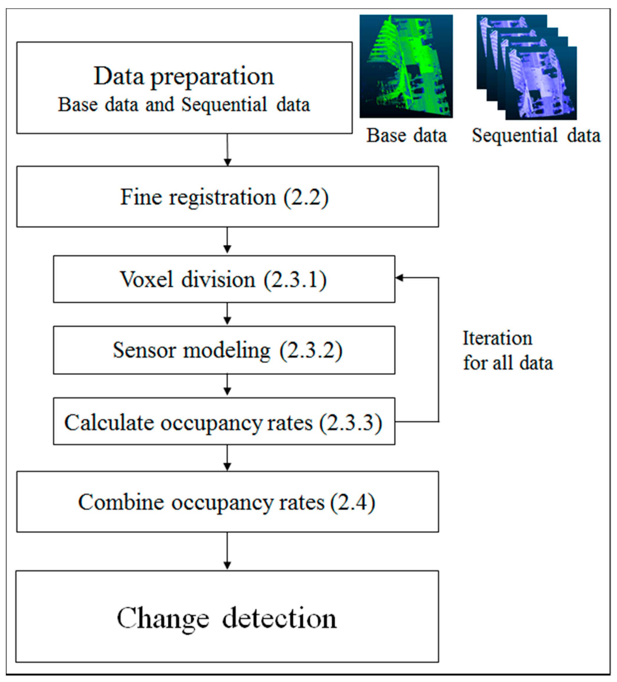
This research utilizes two types of point cloud data. One is acquired using MMS, which is used for building a 3D road map, and data of the second type is obtained from cheap sensors equipped in regular vehicles that have automatic driving or a driver supporting system. The first point cloud is denser and has higher accuracy than the data of the latter type. On the other hand, the data with lower accuracy can be acquired low cost and, more frequently, and has the three characteristics mentioned in Section 1. In this research, we refer to the former as “base data”, and the latter as “sequential data” (Table 1) in observation order. To deal with those characteristics, the proposed method consists of two parts, the registration and the occupancy grid methods (Figure 2). Initially, the sequential data are geometrically corrected and superimposed on the base data in the registration process. We apply the ICP algorithm for this purpose. Since all data used in this study has the same coordinate system, the ICP algorithm can be applied directly. When the data has different local coordinate system, coarse registration will be required to give the initial value for the fine registration such as the ICP algorithm. In the occupancy grid method, the point cloud data space is divided into voxels, and those voxels that contain points from the point cloud are examined. If a voxel includes at least one point, then occupancy rates would be calculated by using a probabilistic sensor model that considers the error of measurement. After occupancy rates are calculated for all data, they will be successively updated by using the calculated result in each part of the data. Finally, based on the changes in the patterns of occupancy rates, the changes in the road environment and tentative changes caused by moving objects are detected and identified.
2.2. Registration
With geometric correction, sequential data are superimposed on the base data. If the gap between the base data and sequential data is large, there would be false identifications of changes even when the road environment has not actually changed. To address this, the registration process is needed before change detection with the occupancy grid method. In this research, we adopt the ICP algorithm. Commonly, before applying a fine registration method like the ICP algorithm, course registration is applied to provide the fine registration method with initial values. However, the sequential data used in this research can be directly applied for fine registration from the experimental results as mentioned in Section 3.2.1. Therefore, we skip the course registration step and directly apply the ICP algorithm in this research.
2.3. Estimation of Occupancy Rate
2.3.1. Occupancy Status at Voxels
The occupancy grid method is applied for change detection. As already stated, some previous research has also applied this method for change detection between two point clouds acquired at different times, but the results contain all differences between the two point clouds, including tentative changes and differences in the measurement area. This research uses only the framework of the occupancy grid method, and calculates occupancy rates in the data obtained from each regular vehicle. Occupancy rates are probabilistic expressions of the occupancy status, and this research follows previous work to calculate these rates [28]. Subsequently, occupancy rates are successively updated by each calculation result to detect only road environment changes.
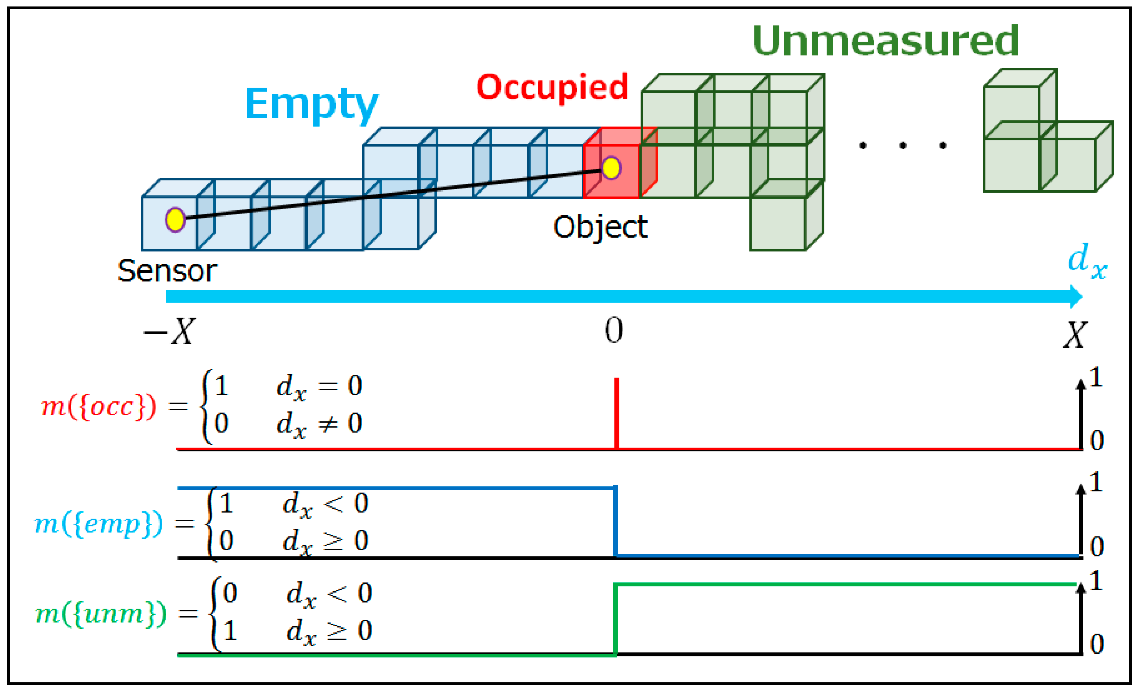
In the first step of the occupancy grid method, the point cloud data space is divided into three-dimensional grids, known as voxels. Following this, the “occupancy status” is defined based on the existence of points from the point cloud in each voxel. Occupancy statuses are classified into three categories: occupied, empty, and unmeasured. A voxel containing at least one point is regarded as “occupied”, because it would contain an object or at least a part of it. When a voxel does not have any points and is included in the observation area, it is labeled as “empty”. If the voxel does not belong to the measurement area of both the base data and sequential data, it is considered “unmeasured”. With the “unmeasured” category, the method can explicitly discriminate between road environment changes and data differences due to measurement ranges. Both empty and unmeasured voxels do not include any points, so an additional method is needed to distinguish between them. Following previous research, Bresenham’s line-drawing algorithm [37] is employed to detect empty voxels. After each point and scanner position is aligned, Bresenham’s line-drawing algorithm calculates the path of the LASER rays from the scanner to the object, and identifies the voxels that the rays pass through. These voxels can be considered empty, and the other voxels are unmeasured. The voxel size should be specified carefully because it has a crucial influence on the result and computational time. As will be explained in Section 3.2.1, the voxel size is set as 0.5 m on a side by taking into account the target size.
2.3.2. Sensor Model
The probabilistic concept of the occupancy status is introduced in preparation for the sensor model. The model considers the measurement error and expresses the probability of each occupancy status in a voxel. Let the probabilistic expression of an occupancy status be called the “occupancy rate” in this research. The occupancy status of a voxel is either empty or occupied in real space. These possibilities can be represented as the universal set U = {emp, occ}, where {emp} and {occ} stand for empty and occupied, respectively. On the other hand, the measurement results are classified empty, occupied and unmeasured. Accordingly, the set of measurement results has to be considered as the power set of U, namely 2U = {, emp, occ, unm}, where {unm} stands for unmeasured. The belief mass m can then be defined as satisfying the following three mathematical conditions:
m: 2U → [0,1],
Equations (1) and (2) are equivalent to the definition of ordinary probabilistic measurement, but Equation (3) is a unique condition of the Dempster–Shafer theory. Equation (3) can be expressed as follows:
m({emp}) + m({occ}) + m({unm}) = 1.
Equation (3) allows us to explicitly consider the ignorance from the lack of information. If other evidence is added, m({unm}) would become small and the difference would be allocated to m({emp}) and m({occ}). Thus, the belief masses m({emp}) and m({occ}) are dynamically calculated. In other words, the uncertainty m({unm}) gradually becomes small, and m({emp}) and m({occ}) are explicitly specified through successive observations. In this research, ignorance or uncertainty from lack of information corresponds to unmeasured from lack of observation. Explicitly examining unmeasured voxels would enable the differentiation between road environment changes and differences in measurement areas.
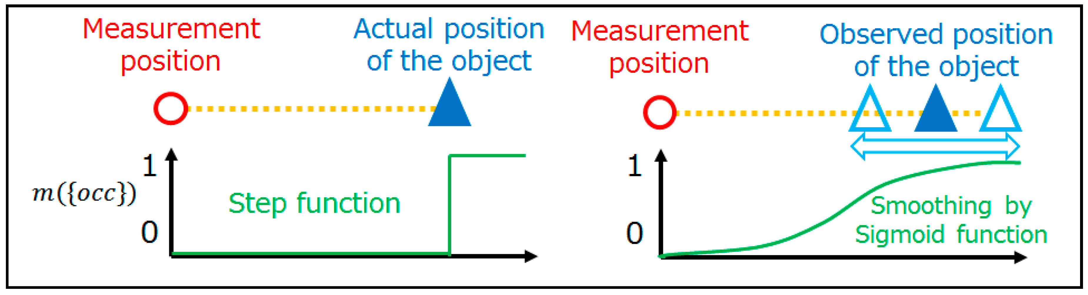
Based on the concept of occupancy rates, the sensor model can be introduced. Before explaining the mathematical expressions of the sensor model, it might be helpful to refer to the ideal situation. If there were no measurement errors involved, the occupancy rates would be expressed as in Figure 3. Each occupancy rate is explicitly classified without fuzziness, and it is easy to distinguish between empty, occupied, and unmeasured voxels. However, there are many errors to be considered in actual measurement. This research considers two types of errors. One is the horizontal direction error of LASER rays, and the other is the vertical direction error. Figure 4 depicts the error in the horizontal direction. In the case of an ideal sensor, the occupancy rate can be represented as a step function. However, a step function is not enough to express the errors in actual measurement. Therefore, a sigmoid function is introduced to represent fuzziness, as sigmoid functions are frequently used for smoothing step functions.
Measurement errors related to the vertical direction also exist. These kinds of errors are caused due to the following reasons: (i) A LASER ray expands like a cone after being launched from the sensor; (ii) the error remains after registration; and (iii) there are other random errors of measurement. A Gaussian distribution is applied for representing such kinds of errors because the LASER used for measurement is often modeled as a Gaussian beam, and other random errors should follow a Gaussian distribution.
2.3.3. Occupancy Rate Calculation
At first, it is necessary to standardize a location in voxels for calculating occupancy rates. The occupancy rates in a voxel are defined as the ones at the center of the voxel in this research. Accordingly, the sensor model also should consider the distance between the center of the voxel and a point. The distance between the center of voxel g and the point location p are considered. The longitudinal distance dx and the transverse distance dy are defined as follows:
where r0 is the unit vector on the line from the sensor to the observed point.
By using two distances dx and dy, the belief mass of each occupancy status at the voxel center g is defined as follows:
The parameter controls the gradual transition from occupied to empty and unmeasured, c corresponds to the fuzziness of the occupied space, and expresses the expansion of the LASER ray.
Generally, there are several points in one voxel. If the voxel contains only one point, then the calculated result would directly represent the occupancy rates of this voxel. However, if there are several points in the voxel, the occupancy rates from each point would be integrated to one value by the Dempster’s rule of combination. In the Dempster’s rule of combination, two belief masses m1 and m2 acquired from independent observations are generally combined by the following equation:
When this rule is applied to this research, Equation (11) can be expressed as follows:
where .
2.4. Change Detection by Transition of Occupancy Rate
For identifying the changes in the road environment, it would be useful to use the dynamic changes of occupancy rates by combination. There are unique patterns of occupancy rate transitions for each difference in the data. After calculating the occupancy rates in each voxel for all data, the occupancy rates are also combined by Dempster’s rule of combination in units of voxels. If any kind of change takes place, the occupancy rates will likewise change.
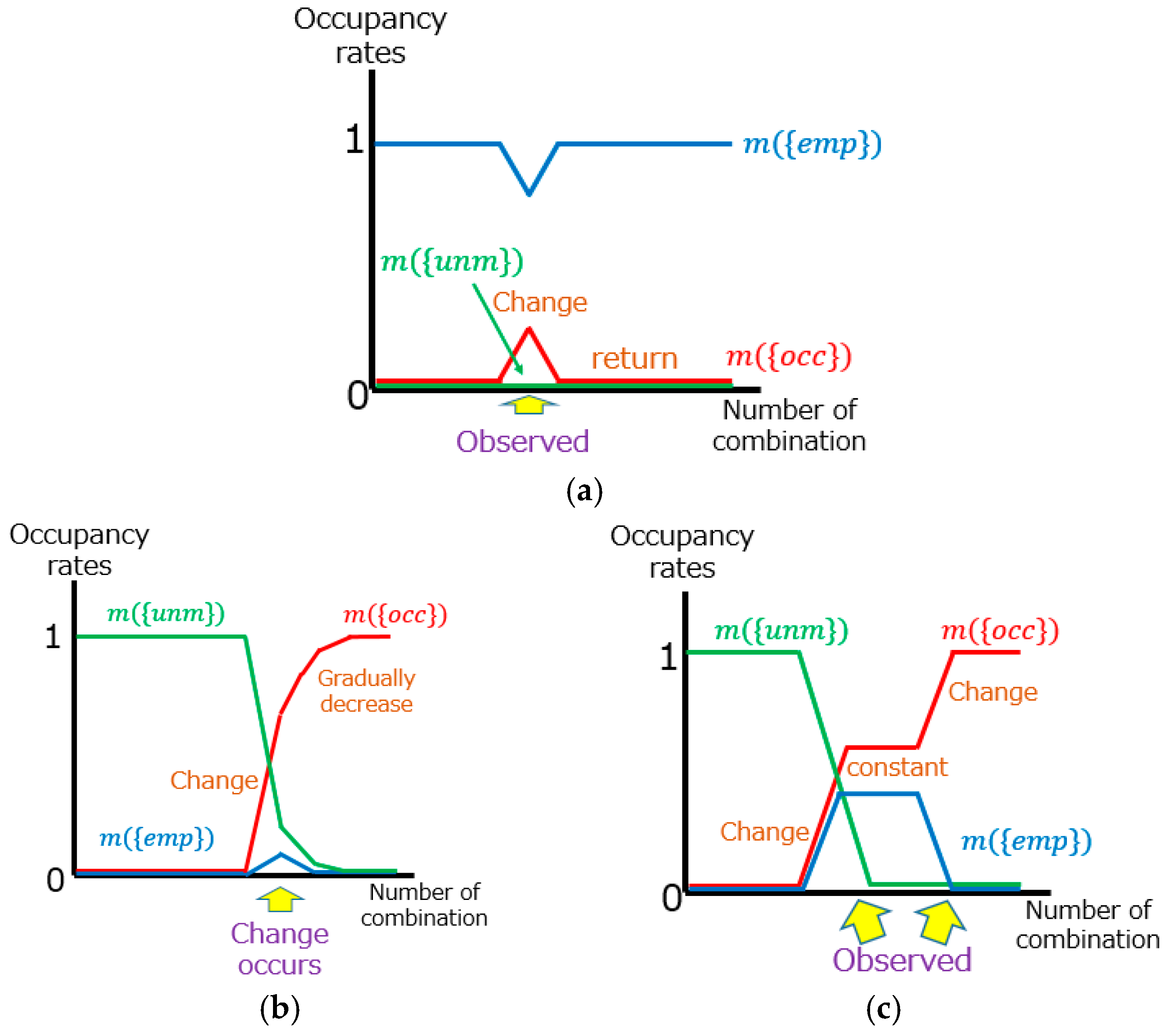
Figure 5 shows the relationship between transitions of occupancy rates and changes in the road environment. As mentioned in Section 2.1, the sequential data are following the order of observation. In the case that some data include tentative changes such as oncoming vehicles or pedestrians, the change of occupancy rates will occur only when the data with tentative changes are combined (Figure 5a). Because the data without tentative changes are combined after the data with tentative changes, the occupancy rates will return to the original state. When a change in the road environment occurs, the occupancy rate will start to change (Figure 5b). In this process, the magnitude of changes in the occupancy rates tend to gradually decrease as each occupancy rate becomes close to 0 or 1. Accordingly, tentative changes and changes in the road environment are identified as follows: In a road environment change, (i) there is a large difference between the original occupancy rate and the final rate; (ii) the occupancy rate does not return; and (iii) the magnitude of change in the occupancy rate gradually decreases. Moreover, the areas observed with some sequential data show changes in the occupancy rate only when the data measuring those areas are combined, and, otherwise, the rates do not change (Figure 5c). Information on sensor specifications and measurement paths allow us to find the places that are observed in some sequential data. The occupancy rates change only when vehicles pass through those places. Therefore, if the occupancy rates change only in specific data, these changes would have happened not because of road environment changes but due to different measurement areas. By using these three patterns, it is possible to distinguish the road environment changes from other changes.
3. Results
3.1. Data
3.1.1. Specification of Data
Two kinds of point cloud data are considered in this research. One is acquired using MMS for building the 3D road map, and another is sequential data that is routinely acquired by regular vehicles. However, current vehicles do not yet capture such sequential data. Therefore, for the purpose of this study, sequential data are synthetically created from the base data. The base data was acquired using Nikon-Trimble’s MX-5 (Tokyo, Japan), which is equipped with GNSS (Global Navigation Satellite System) and IMU (Inertial Measurement Unit) measuring devices, POS (Position and Orientation System) LV 520 (Applanix, Richmond Hill, Canada), and one LASER scanner, the Riegl VQ 450 (Horn, Austria). The area of interest is the intersection in Umeda, Osaka Prefecture, Japan. The specifications for sequential data were decided by referring to sensors released several years ago. Sequential data would contain position and rotation errors, their densities would be lower, and their measurement ranges would be narrow in comparison with base data. In addition, the specifications of sequential data would vary because these data are acquired by different vehicles. However, it is almost impossible to precisely estimate sensor specifications of the future, so this research considers only two kinds of sequential data. Here, we refer to the two sets of sequential data as (A) and (B), and assume that (A) has higher performance than (B). The differences between (A) and (B) can be expressed in four variables: position accuracy, angle accuracy, point density and measurement range. It is important to point out here that the data from cheap sensors are acquired more frequently. According to the above assumptions, the specifications of the two sets of sequential data are decided as shown in Table 2. Both sets of sequential data are created as follows: first, position and angle errors are added to the base data. Next, their point densities are lowered. Finally, a part of the measurement area is cut.
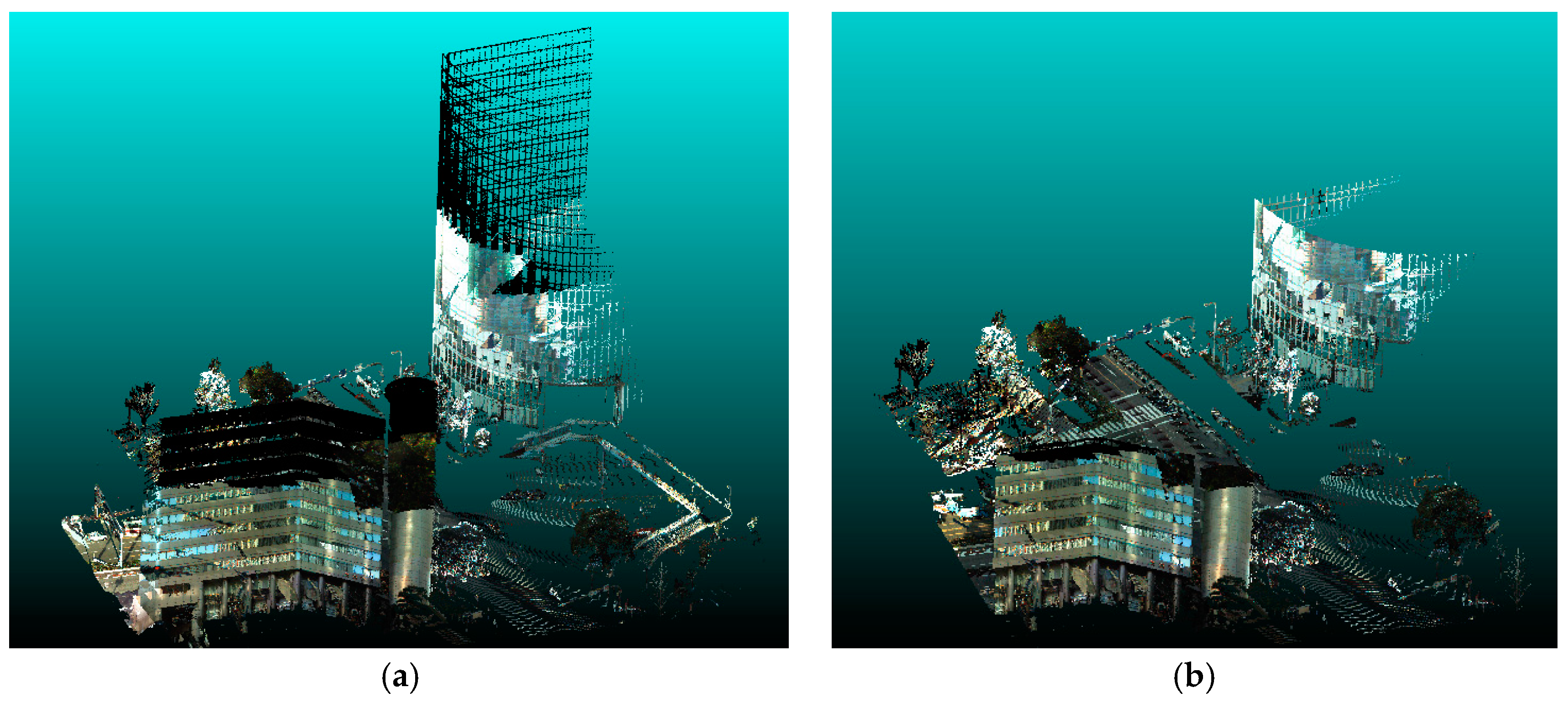
The measurement areas in the data vary due to two reasons. The first is due to the various trajectories of vehicles. If some vehicles measure certain areas, others might not measure those areas. In addition, the varieties of sensors have an influence on the measurement areas. Higher performance sensors would cover wider ranges, and these differences are caused by different performances in terms of distance and angle measurement. This experiment considers different measurement areas in the horizontal and vertical directions. The former corresponds to the trajectory difference and the performance difference in terms of distance, and the latter corresponds to the difference in angle measurement. Figure 6 shows the plan view of the area of interest. The base data can cover the whole area, but sequential data can only measure a part of it, and sequential data (A) and (B) have different measurement ranges. Similarly, Figure 7 shows an elevated view of the area of interest. Base data and sequential data (A) are set so as to measure the same range, while sequential data (B) has a narrow range.
3.1.2. Road Environment Change and Tentative Change
Based on the degree of change, two scenarios are considered in the experiment. The first is the large-scale change scenario, in which the road structure, such as the width of the roadway, is changed. The second is the small-scale change scenario, in which some road features such as pole structures and signboards are changed. The location and changed features are shown in Figure 8 and Table 3, respectively.
Data acquired at different times is likely to contain tentative changes. Pedestrians and oncoming cars are added to and removed from base data. The shadow area would also change when tentative changes occur. However, the data used contain errors in corresponding points and vehicle trajectories, so the parts that fall in shadow areas are expressed only when they can be easily and clearly reconstructed. In order to decide the number of pedestrians and vehicles to account for in our study, we refer to the 2010 transportation census of the Osaka Prefecture. Since we only have base data as of today, tentative changes are synthetically added to sequential data.
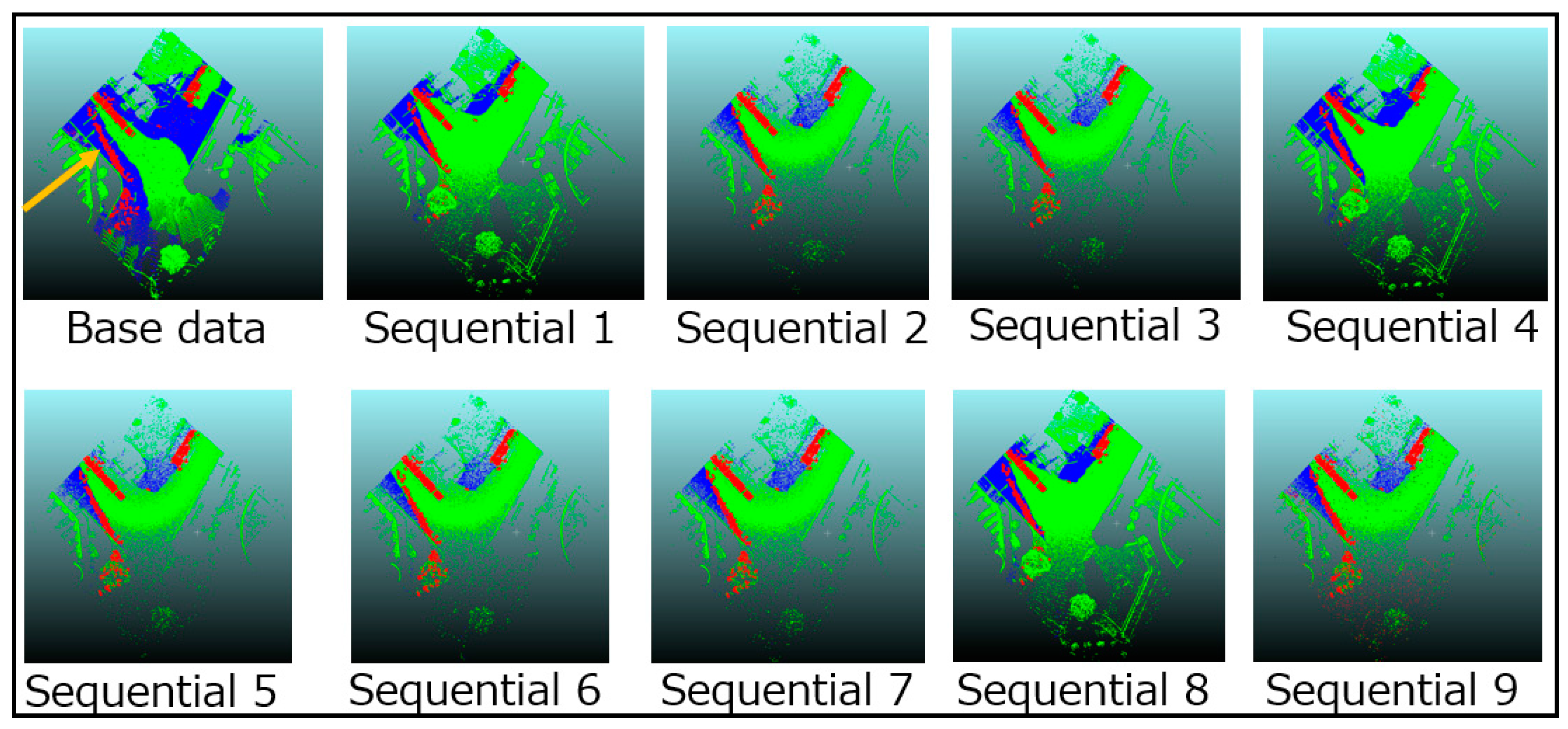
We prepared a total of ten instances of data for change detection in each scenario. The first data instance is the base data, and the others are sequential data. All instances of sequential data contain tentative changes, and just four of the nine data instances record road environment changes. Performances of sequential data, (A) and (B), are randomly set in the nine data instances called sequential data number because the data would be acquired randomly by different sensors in realistic situations. The number of data and observed changes are shown in Table 4. Moreover, it is assumed that there is prior knowledge on which data contain road environment changes. While this assumption might seem to be strong, it was difficult to carry out change detection in the pilot experiment without any prior knowledge. Accordingly, it is assumed to be a given that road environment changes are observed in sequential data numbers 6, 7, 8, and 9 in this experiment.
3.2. Experimental Results
3.2.1. Parameters Setting
The ICP algorithm is implemented by using the Point Cloud Library (PCL) [16]. The distance for finding corresponding points is set as 0.1 m for all data, and the number of iterations for each data instance is decided based on pilot trials. The size of voxels is a crucial factor in change detection because it determines the resolution and minimum size of detectable change. In this experiment, voxels are set as 0.5 m × 0.5 m × 0.5 m cubes to detect small road objects. The parameters of the sensor model also have a significant influence on the results. In this study, we arrive at the values of the parameters experimentally and verify the effectiveness according to previous research. This experiment considers three kinds of data: base data, sequential data (A) and sequential data (B). For each kind of data, the parameters are set as = (8,10,6), (10,8,12), (20,10,18). In this paper, the tendency of the relationship between the parameters and occupancy rates is examined through trial and error. These parameter values are decided for the purpose of making occupancy rates different in each kind of data.
3.2.2. Registration
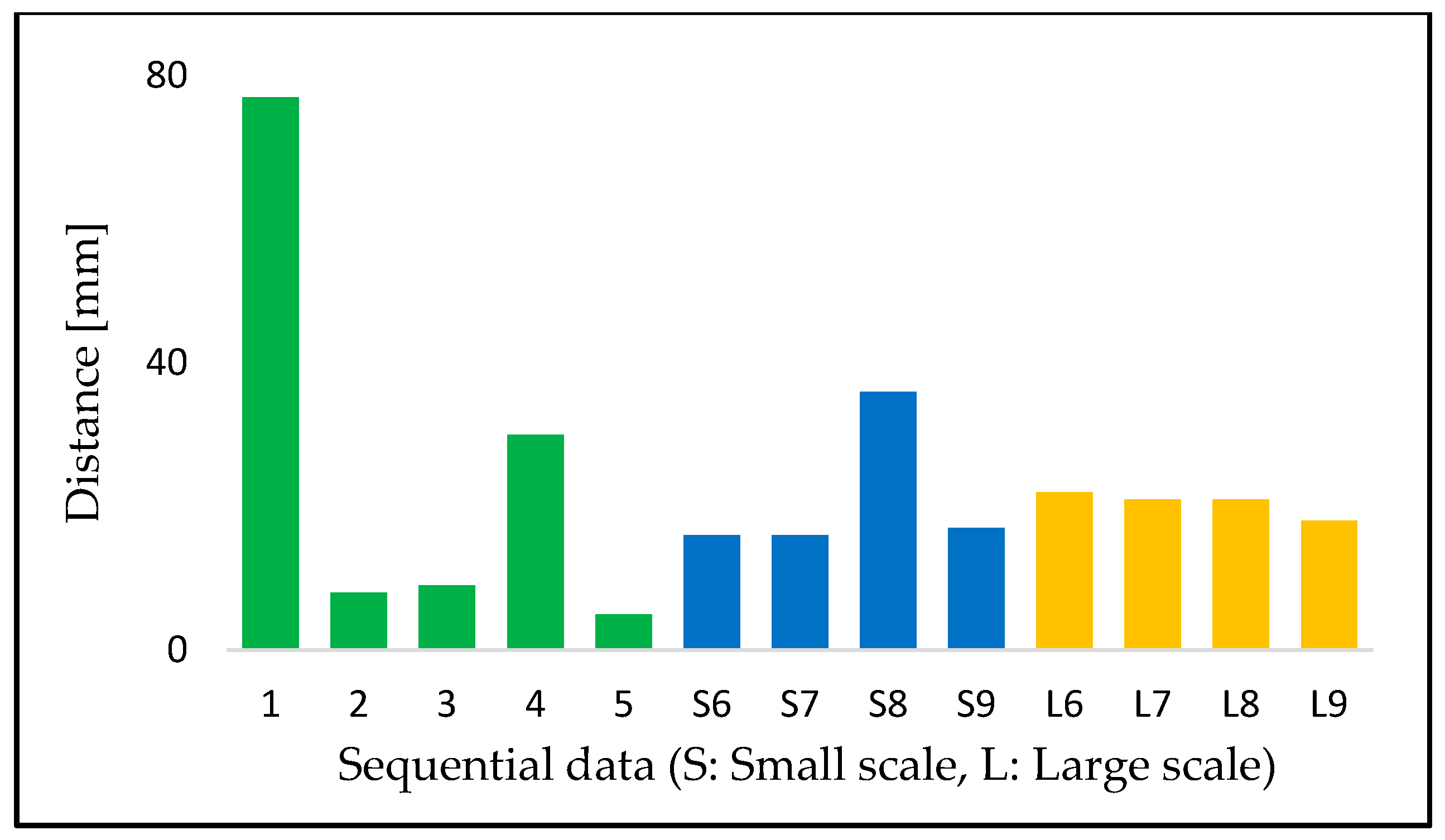
The registration results are shown in Figure 9. The cloud-to-cloud distance is used for evaluating the results. This distance is the nearest neighbor distance between two point clouds, and the base data is used as a reference. This experiment uses the standard function implemented in Cloud Compare [38] to measure the distance.
3.2.3. Tentative Changes and Differences of Measurement Areas
Before examining the detection of road environment changes, we refer to the results for tentative changes and differences of measurement areas. The results for tentative change are shown in Table 5. The sequential data number 9 (performance (B)) is included in calculation, but the result is excluded from Table 5 because the occupancy rates do not change after combination of final data and change detection is impossible. The criteria for determining whether an identification is correct or incorrect is as follows. If at least one voxel recognizes the tentative change as a road environment changes, then the result is a failure. Otherwise, the detection is a success. Next, Figure 10 shows the results for measurement differences. The figure captures the change of occupancy status to occupied after the correcting process has been applied, as mentioned later. The horizontal and vertical differences are successfully prevented from being misclassified.
3.2.4. Road Environmental Change
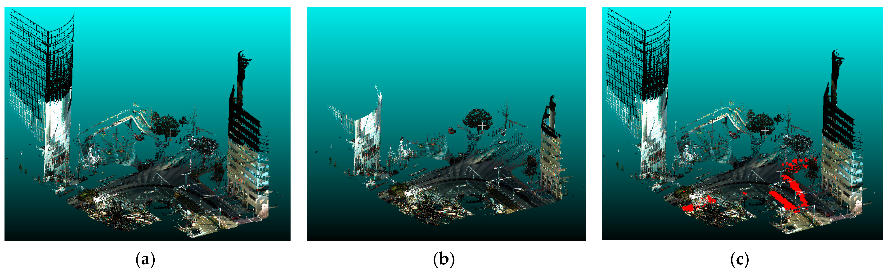
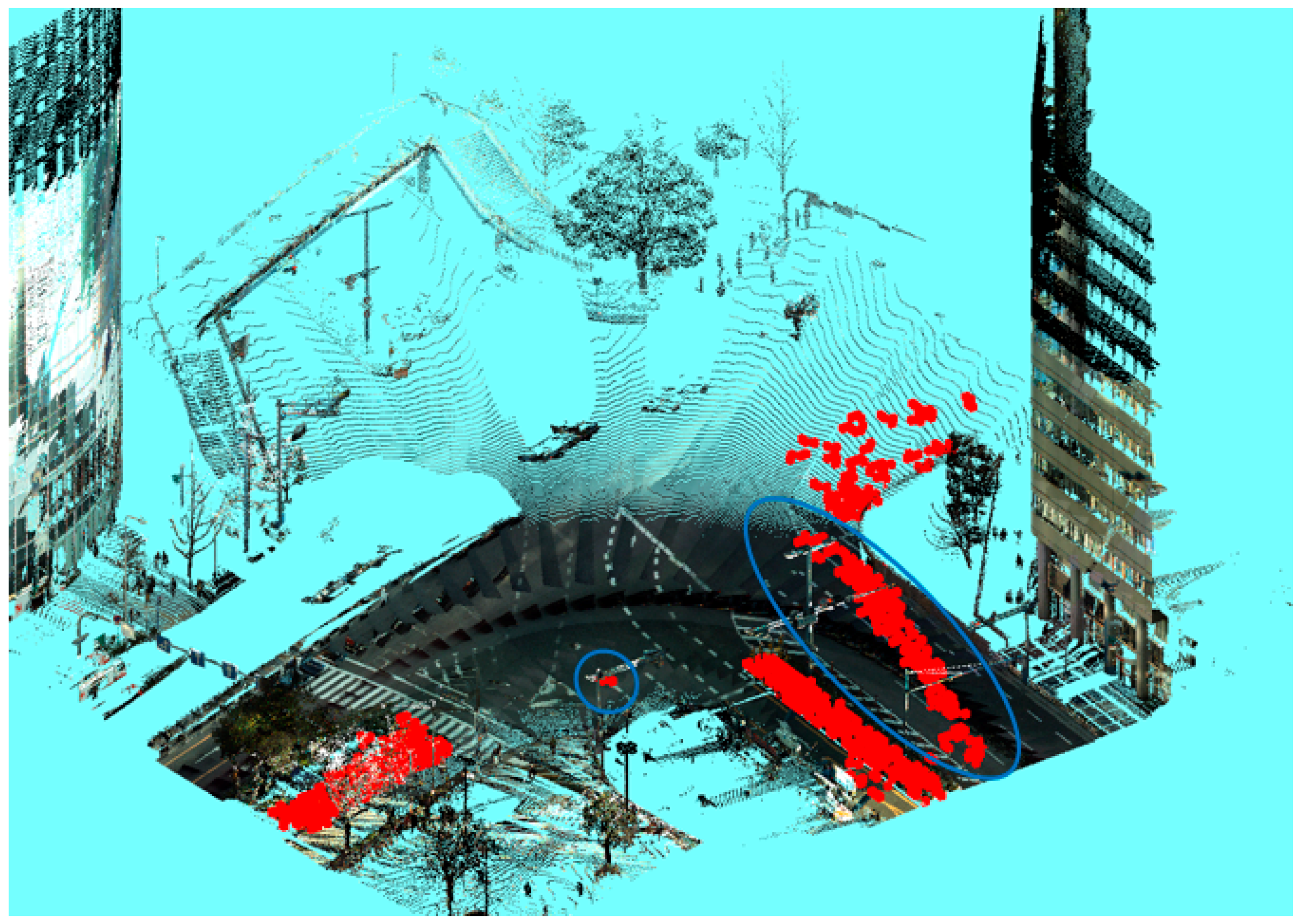
Three out of four road environment changes, called large-scale changes in this paper, are successfully detected. Two of these changes are expansions of the median strip, and the other is a change from street-side trees to a roadway. However, there are many excessive and incorrect detections as shown in Figure 11, and it is difficult to isolate only road environment changes. Figure 11 only visualizes the results for which the occupancy status has changed to occupied, but results for the change to empty also contain quite a few misdetections. Therefore, a correcting process is needed for dealing with incorrect detections. A large number of misclassified voxels have the following characteristics. The first is that they are distributed discretely. In other words, they have few neighboring voxels. Second, the incorrect classification is frequently observed in areas where the density is low, such as the area far from the MMS trajectory and behind plantings or fences. A voxel that satisfies the following conditions is removed in the correcting process: (i) the number of voxels neighboring the voxel is less than three; (ii) the area behind plantings or fences; (iii) the area is not within the roadway. After applying the correcting process, the results significantly improved (Figure 12). However, the area marked by the blue ellipse still contains incorrect detections.
The results for small changes, such as in the road structure, are mainly divided into four categories as in Table 6. The table represents the real environment states in the first and third columns, and the observation state in the second column. If an object originally exists but is occluded, then the first column is occupied, and the second column is unmeasured. Pattern (a) is a change to empty, and the detection failure in which only a part or nothing of the object is correctly detected is frequently observed. Pattern (b) is observed when the occupied or empty voxels change to unmeasured. In this pattern, the occupancy rates do not change at all, so these kinds of changes cannot be detected by the proposed method. Pattern (c) is a change from empty to occupied, and there can be a detection failure here like in pattern (a). On the other hand, in pattern (d), when an unmeasured area in the base data changes to occupied, good results can be acquired. However, there are areas where there can be an over-detection, which makes it difficult to isolate only the changed area, and therefore additional correcting processing is needed.
4. Discussion
4.1. Registration
The registration results ranged from 5 mm to 70 mm in terms of cloud-to-cloud distance. The interpretation of registration results is not straightforward because there are no theoretical relationships between registration performance and the results of change detection. When there remain such large gaps after registration, the change detection might not be expected to succeed. However, the size of voxels and the data specifications also have a significant influence on the results of change detection. Moreover, the size and shape of the target objects also influence the result. Considering these issues, the performance of the registration process must be evaluated based on the results of change detection. Figure 12 shows one incorrect detection due to an error left behind by the registration process, as mentioned in Section 4.2.2.
The results for sequential data (A) tended to be poorer than those for sequential data (B), especially sequential data 1 while data (A) is denser and covers a broad area. The reasons are not clear from the assessments based only on this experiment, but some of the poor results might occur because data (A) tend to fall into a local solution. Moreover, the relationship between the density and results of the registration process could be due to the evaluation method. This experiment uses the cloud-to-cloud distance, but there are other methods to calculate the distance between two-point clouds. Future work must explore other methods for evaluating registration results.
4.2. Change Detection
4.2.1. Different Measurement Areas and Tentative Changes
As shown in Figure 12, the areas that were recorded only in the base data and sequential data (A) can be successfully identified and incorrect classifications can be avoided. Among sequential data numbers 6, 7, 8, and 9, only data number 8 has a wide measurement range (performance (A)), and there were areas labeled unmeasured in sequential data numbers 6, 7 and 9, which only sequential data number 8 could measure. As a result, there are no incorrect detections, and this demonstrates the importance and effectiveness of explicitly defining the “unmeasured” occupancy status.
With regards to tentative changes, Table 5 shows that incorrect classifications occur when objects are added and appear. These areas are regarded as unmeasured, except for the parts with tentative changes. When m({occ}) increases, the occupancy rates do not return when m({unm}) = 1 is combined.
On the other hand, the results for removals or disappearances are good. However, these results should be interpreted carefully. Initially, if an object is removed and the corresponding area becomes unmeasured, the occupancy rates would not change at all. As a result, the occupancy of the area might not have changed, although the object is actually removed. Secondly, low point densities tend to improve m({emp}) or m({unm}) and suppress m({occ}) before real changes occur, so the removal or disappearance of objects does not have any influence on the occupancy rates. Due to this, the voxel also does not show a transition in its occupancy rates. Therefore, we must be careful while interpreting this result, and more explicit methods of evaluation are needed in the future.
4.2.2. Large-Scale Change Scenarios and Correcting Processes
Three out of four changes can be successfully detected by the proposed method. These areas change from unmeasured to occupied, so it shows clear changes in the occupancy rates, and the smaller effect of point density. If smaller changes need to be detected, or more detail is needed in the detected changes, it would be effective to make the size of the voxels smaller. However, using smaller voxels increases the calculation time because the number of voxels also increases. Thus, the size of the voxels should be determined by considering the potential tradeoffs between accuracy and calculation cost.
As mentioned in Section 3.2.4, a correcting process is needed to improve the visibility so that we can easily and accurately recognize road environment changes. The main cause of misdetection is low density in the point cloud data. In particular, the point cloud tends to be sparse in the areas behind plants or fences, and far from the trajectory of vehicles. Due to this, sequential data in these areas have low densities and this leads to misclassifications. In this research, additional processing is applied and most of these misclassifications can be successfully removed. This process is manually executed in this experiment, but it is also be possible to implement this automatically. However, the extent to which this correcting process can be applied in other situations must be examined in future work. The removal conditions were decided ad hoc for this experiment, so it is necessary to establish more general processes and methods in the future. In addition, when similar processing is applied in the small-scale scenario, small objects are also removed because they are contained in only a few voxels. Further examination and research on reducing incorrect detections are needed in the future.
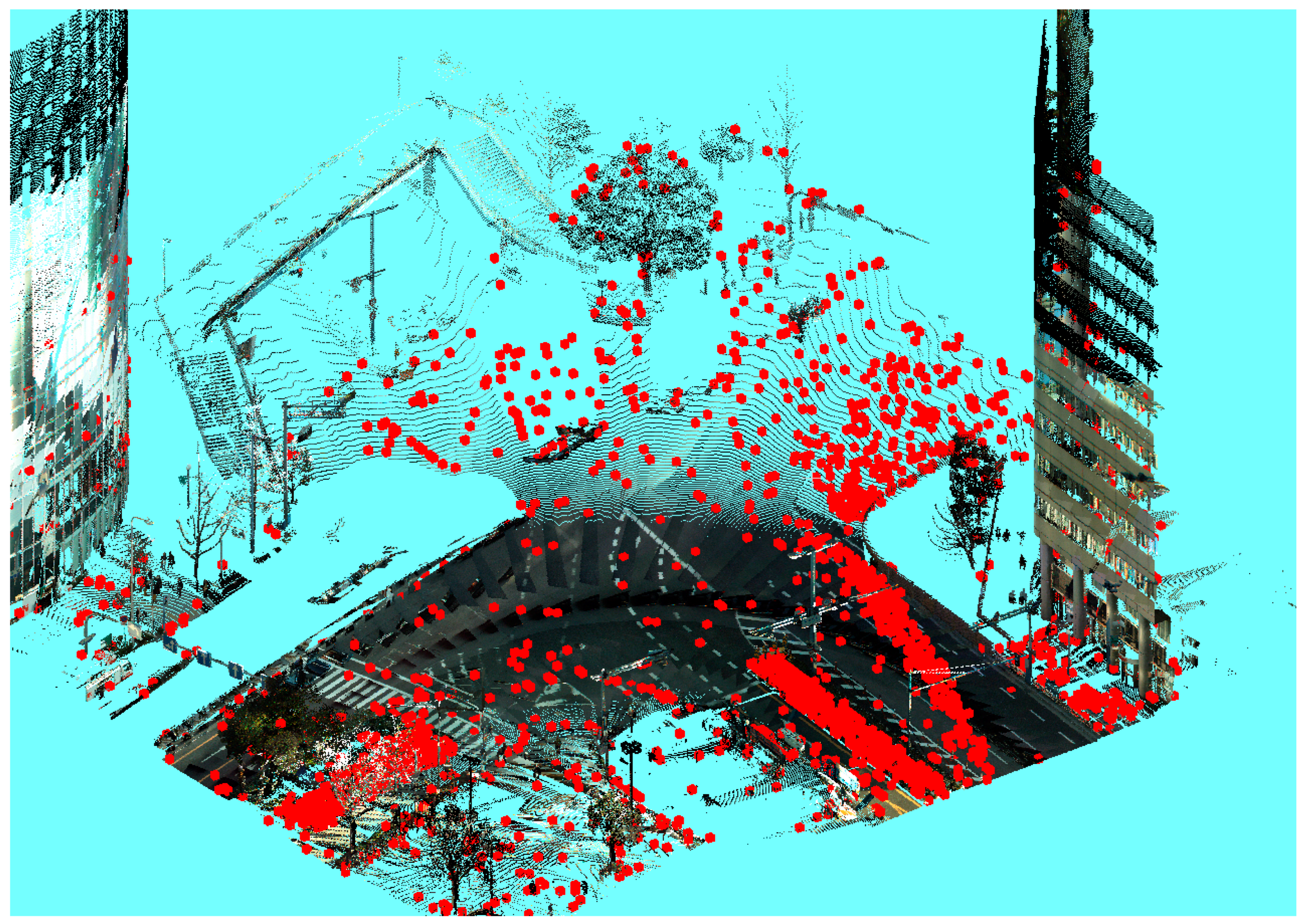
Even after applying additional processing, some areas and objects were still incorrectly detected. At first, the removal of the median strip could not be detected well. The reason for this could be that the height of the median strip is much lower than the voxel size of 0.5 m, and the occupancy rates do not change due to low density. Secondly, the misclassifications remain shown in two blue circles in Figure 12. The incorrect result in small circles can be regarded as errors. It is quite difficult to distinguish the areas in large circles from misclassification. The broad area in Figure 12 is incorrectly recognized to be changed to occupied. The transitions of occupancy rates show that rates in this area mainly changed when sequential data numbers 6 and 7 (both performance (B)) were combined, even though the registration results in Figure 9 are not worse than in other data. Figure 13 shows the elevation distribution of the base and sequential data after registration as seen from above. The red parts are detection results that changed to occupied. The elevation of the blue parts is less than 3.23 m, and that of the green parts is higher than 3.23 m. 3.23 m is the boundary height between voxels in this experiment. The areas incorrectly detected fall in the blue parts, except in sequential data numbers 6 and 7. Therefore, this area is covered by voxels in sequential data numbers 6 and 7, and that, as a result, changes occupancy rates. We thus infer that errors after registration cause this large incorrect detection. This experiment uses cloud-to-cloud distances for evaluating registration results, but this misdetection implies that this criterion is insufficient. If registration is perfect and two point clouds are completely aligned with each other, the distance should be zero. Thus, the distance between the point clouds represents the error after registration. However, this error can be divided into translation and rotation errors, and this misdetection is likely to be caused by the latter. We therefore suggest that there should be evaluation criteria for registration that explicitly consider the rotation error.
4.2.3. Small-Scale Change Scenario
The change from unmeasured to occupied is well detected (pattern (d)). When high m({occ}) is combined with an unmeasured area, the change in the occupancy rate clearly appears. Moreover, even if some points are not included in a voxel due to low point density, the occupancy rates remain because occupancy rates stay constant when m({unm}) = 1 is combined. In other words, pattern (d) is robust case against point density. However, the change from occupied to empty (pattern (a)) and the change from empty to occupied (pattern (c)) are not always detected well. Theoretically, the occupancy rates should change after road environment changes occur. However, m({emp}) or m({unm}) become high in many voxels even before road objects actually disappear in pattern (a). This phenomenon is thought to be caused by low point density. The number of points in a voxel becomes small even if the voxel corresponds to an occupied area. m({occ}) becomes significantly small before a change to empty happens and it disturbs the change detection by using transition of occupancy rates. Similarly, pattern (c) also contains a detection failure. Theoretically, m({occ}) should begin to increase and m({emp}) decrease after a change to occupied happens. However, m({occ}) is not always large in sequential data numbers 6, 7, 8, and 9 that include road environment changes because of low point density. Thus, the occupancy rates do not change as expected, and detection failure occurs. Selecting which data are used for change detection can be an effective solution to detection failures such as in pattern (a) and pattern (c). The main cause of misdetection is low point density, and the results are expected to improve if we use denser data from high performance sensors. This approach is not unreasonable because it is possible to have the sensor specifications along with the acquired data.
On the other hand, it is practically impossible to detect changes to unmeasured (pattern (b)). When the occupied area become unmeasured, only m({unm}) = 1 is combined and rates do not change at all. The proposed method depends on changes in the occupancy rates, so it cannot detect changes that are not related to transitions of occupancy rates. While the experiment does not consider change from empty to unmeasured, it is also impossible to detect any changes by the proposed method. Using other data acquired from different trajectories and angles might be effective in detecting these changes. However, this cannot be said to be a limitation of the proposed method, and further research and methods are left as future work.
5. Conclusions
In this paper, we proposed a change detection method by using low accuracy but high frequency point cloud data. The proposed method is a series of steps from registration to the visualization of the results. Much of the prior research work tended to focus on sensors with same specifications. The method that we propose deals with map updating in more realistic situations. A novel contribution of this work is the use of occupancy rate transitions through a series of multiple point clouds to discriminate real changes from tentative changes. The experimental results demonstrate that the proposed method can distinguish the real changes from other differences in the data. Moreover, we reflect on the relationship between registration and change detection, and infer that the evaluation criteria for registration must specifically consider rotation error.
There remain several challenges associated with this method for future researchers to address. The voxel size is assumed to be homogeneous in this study. It can be extended to the heterogeneous sized voxel such as octrees, and then it leads to more efficient and effective methods for huge amounts of data. The sensor model and parameters were selected experimentally. Further consideration towards the development of the sensor model is required, so that the model might directly influence the results of change detection. In addition, while the parameters were specified experimentally, the automatic specification of parameters and detailed sensitivity analysis are needed. For this purpose, the machine learning method will be expected. Furthermore, methods to improve the rate of correct detection are important. In this experiment, similarities were found in the areas that were incorrectly detected, which made it possible to apply additional processes to rectify the incorrect detections. However, it might not always be possible to find such similarities. Therefore, future work must look to improve the proposed method independent of these similarities. Finally, we need to gather good quantities of realistic data that we can use in developing methods for detecting various objects in the street. The data to be provided by cheap sensors were manually created for the experiment in this work because such sensors do not exist at present. The synthetic data do not explicitly take into account error or noise against measurement. Such kind of error or noise will be included in order to generate more realistic data. We need to have data from various street environments and objects, as regular vehicles will be equipped with various sensors in actual traffic situations. The proposed method should be applied to real data to confirm significance of the method. Thus, additional experiments in other situations are required. After dealing with the various challenges expressed above, we can expect this research work to turn into a practical reality, and enable sustainable updating and applications of 3D road maps.
Acknowledgments
The point cloud data and aerial images used in this study were provided by the PASCO CORPORATION (Tokyo, Japan). We would like to express our gratitude for their cooperation. We shall also express our thanks to anonymous reviewers and editors for their constructive and useful comments.
Author Contributions
Takashi Fuse conceived the idea of and designed the study. Naoto Yokozawa analyzed the data and conducted the experiments. All authors contributed to the preparation of the manuscript.
Conflicts of Interest
The authors declare no conflict of interest.
References
- Shimada, H.; Yamaguchi, A.; Takada, H.; Sato, K. Implementation and Evaluation of Local Dynamic Map in Safety Driving Systems. J. Transp. Technol. 2015, 5, 102–112. [Google Scholar] [CrossRef]
- Moravec, H.; Elfes, A. High resolution maps from wide angle sonar. In Proceedings of the IEEE International Conference on Robotics and Automation, St. Louis, MO, USA, 25–28 March 1985; Volume 2, pp. 116–121. [Google Scholar]
- Dempster, A.P. Upper and Lower Probabilities Induced by a Multivalued Mapping. Ann. Math. Stat. 1967, 38, 325–339. [Google Scholar] [CrossRef]
- Shafer, G. A Mathematical Theory of Evidence; Princeton University Press: Princeton, NJ, USA, 1976; ISBN 978-0-691-10042-5. [Google Scholar]
- Scovanner, P.; Ali, S.; Shah, M. A 3-dimensional sift descriptor and its application to action recognition. In Proceedings of the 15th ACM International Conference on Multimedia, Augsburg, Germany, 25–29 September 2007; ACM: New York, NY, USA, 2007; pp. 357–360. [Google Scholar]
- Lowe, D.G. Distinctive image features from scale-invariant keypoints. Int. J. Comput. Vis. 2004, 60, 91–110. [Google Scholar] [CrossRef]
- Sipiran, I.; Bustos, B. Harris 3D: A robust extension of the Harris operator for interest point detection on 3D meshes. Vis. Comput. 2011, 27, 963–976. [Google Scholar] [CrossRef]
- Guo, Y.; Bennamoun, M.; Sohel, F.; Lu, M.; Wan, J.; Kwok, N.M. A Comprehensive Performance Evaluation of 3D Local Feature Descriptors. Int. J. Comput. Vis. 2016, 116, 66–89. [Google Scholar] [CrossRef]
- Hashimoto, M. 3D Features for point cloud data processing. Presented at the DIA2015 Workshop, Hiroshima, Japan, 5–6 March 2015; Intelligent Sensing Laboratory, Chukyo University: Nagoya, Japan, 2015. Available online: http://isl.sist.chukyo-u.ac.jp/Archives/archives-e.html (accessed on 19 October 2017).
- Johnson, A.E.; Hebert, M. Using spin images for efficient object recognition in cluttered 3D scenes. IEEE Trans. Pattern Anal. Mach. Intell. 1999, 21, 433–449. [Google Scholar] [CrossRef]
- Rusu, R.B.; Blodow, N.; Marton, Z.C.; Beetz, M. Aligning point cloud views using persistent feature histograms. In Proceedings of the IEEE/RSJ International Conference on Intelligent Robots and Systems, Nice, France, 22–26 September 2008; pp. 3384–3391. [Google Scholar]
- Rusu, R.B.; Blodow, N.; Beetz, M. Fast Point Feature Histograms (FPFH) for 3D registration. In Proceedings of the IEEE International Conference on Robotics and Automation, Kobe, Japan, 12–17 May 2009; pp. 3212–3217. [Google Scholar]
- Tombari, F.; Salti, S.; Di Stefano, L. Unique signatures of histograms for local surface description. In Proceedings of the European Conference on Computer Vision, Crete, Greece, 5–11 September 2010; Springer: Berlin, Germany, 2010; pp. 356–369. [Google Scholar]
- Drost, B.; Ulrich, M.; Navab, N.; Ilic, S. Model globally, match locally: Efficient and robust 3D object recognition. In Proceedings of the IEEE Computer Society Conference on Computer Vision and Pattern Recognition, San Francisco, CA, USA, 13–18 June 2010; pp. 998–1005. [Google Scholar]
- Tombari, F.; Salti, S.; Stefano, L.D. A combined texture-shape descriptor for enhanced 3D feature matching. In Proceedings of the 18th IEEE International Conference on Image Processing, Brussels, Belgium, 11–14 September 2011; pp. 809–812. [Google Scholar]
- Point Cloud Library (PCL). Available online: http://pointclouds.org/ (accessed on 19 October 2017).
- Hänsch, R.; Weber, T.; Hellwich, O. Comparison of 3D interest point detectors and descriptors for point cloud fusion. ISPRS Ann. Photogramm. Remote Sens. Spat. Inf. Sci. 2014, 2, 57–64. [Google Scholar] [CrossRef]
- Kim, H.; Hilton, A. Evaluation of 3D Feature Descriptors for Multi-modal Data Registration. In Proceedings of the International Conference on 3D Vision—3DV, Seattle, WA, USA, 29 June–1 July 2013; pp. 119–126. [Google Scholar]
- Salvi, J.; Matabosch, C.; Fofi, D.; Forest, J. A review of recent range image registration methods with accuracy evaluation. Image Vis. Comput. 2007, 25, 578–596. [Google Scholar] [CrossRef]
- Besl, P.J.; McKay, N.D. A method for registration of 3-D shapes. IEEE Trans. Pattern Anal. Mach. Intell. 1992, 14, 239–256. [Google Scholar] [CrossRef]
- Chen, Y.; Medioni, G. Object modeling by registration of multiple range images. In Proceedings of the IEEE International Conference on Robotics and Automation, Sacramento, CA, USA, 9–11 April 1991; Volume 3, pp. 2724–2729. [Google Scholar]
- Turk, G.; Levoy, M. Zippered Polygon Meshes from Range Images. In Proceedings of the 21st Annual Conference on Computer Graphics and Interactive Techniques, SIGGRAPH ’94, Orlando, FL USA, 24–29 July 1994; ACM: New York, NY, USA, 1994; pp. 311–318. [Google Scholar]
- Masuda, T.; Sakaue, K.; Yokoya, N. Registration and Integration of Multiple Range Images for 3-D Model Construction. In Proceedings of the 13th International Conference on Pattern Recognition, Vienna, Austria, 25–29 August 1996; Volume 1, pp. 879–883. [Google Scholar]
- Rusinkiewicz, S.; Levoy, M. Efficient variants of the ICP algorithm. In Proceedings of the Third International Conference on 3-D Digital Imaging and Modeling, Quebec City, QC, Canada, 28 May–1 June 2001; pp. 145–152. [Google Scholar]
- Qin, R.; Gruen, A. 3D change detection at street level using mobile laser scanning point clouds and terrestrial images. ISPRS J. Photogramm. Remote Sens. 2014, 90, 23–35. [Google Scholar] [CrossRef]
- Girardeau-Montaut, D.; Roux, M.; Marc, R.; Thibault, G. Change detection on points cloud data acquired with a ground laser scanner. In Proceedings of the International Archives of the Photogrammetry, Remote Sensing and Spatial Information Sciences, Enschede, The Netherlands, 12–14 September 2005; p. W19. [Google Scholar]
- Hebel, M.; Arens, M.; Stilla, U. Change detection in urban areas by direct comparison of multi-view and multi-temporal ALS data. In Photogrammetric Image Analysis; Stilla, U., Rottensteiner, F., Mayer, H., Jutzi, B., Butenuth, M., Eds.; Springer: Berlin, Germany, 2011; pp. 185–196. [Google Scholar]
- Hebel, M.; Arens, M.; Stilla, U. Change detection in urban areas by object-based analysis and on-the-fly comparison of multi-view ALS data. ISPRS J. Photogramm. Remote Sens. 2013, 86, 52–64. [Google Scholar] [CrossRef]
- Xiao, W.; Vallet, B.; Paparoditis, N. Change Detection in 3D Point Clouds Acquired by a Mobile Mapping System. ISPRS Ann. Photogramm. Remote Sens. Spat. Inf. Sci. 2013, II-5/W2, 331–336. [Google Scholar] [CrossRef]
- Xiao, W.; Vallet, B.; Brédif, M.; Paparoditis, N. Street environment change detection from mobile laser scanning point clouds. ISPRS J. Photogramm. Remote Sens. 2015, 107, 38–49. [Google Scholar] [CrossRef]
- Thrun, S.; Burgard, W.; Fox, D. Probabilistic Robotics; MIT Press: Cambridge, MA, USA, 2005; ISBN 978-0-262-20162-9. [Google Scholar]
- Hackett, J.K.; Shah, M. Multi-sensor fusion: A perspective. In Proceedings of the IEEE International Conference on Robotics and Automation, Cincinnati, OH, USA, 13–18 May 1990; Volume 2, pp. 1324–1330. [Google Scholar]
- Puente, E.A.; Moreno, L.; Salichs, M.A.; Gachet, D. Analysis of data fusion methods in certainty grids application to collision danger monitoring. In Proceedings of the International Conference on Industrial Electronics, Control and Instrumentation (IECON ’91), Kobe, Japan, 28 October–1 November 1991; Volume 2, pp. 1133–1137. [Google Scholar]
- Kulchandani, J.S.; Dangarwala, K.J. Moving object detection: Review of recent research trends. In Proceedings of the International Conference on Pervasive Computing (ICPC), Pune, India, 8–10 January 2015; pp. 1–5. [Google Scholar]
- Deymier, C.; Chateau, T. IPCC algorithm: Moving object detection in 3D-Lidar and camera data. In Proceedings of the IEEE Intelligent Vehicles Symposium (IV), Gold Coast, Australia, 23–26 June 2013; pp. 817–822. [Google Scholar]
- Yan, J.; Chen, D.; Myeong, H.; Shiratori, T.; Ma, Y. Automatic Extraction of Moving Objects from Image and LIDAR Sequences. In Proceedings of the 2nd International Conference on 3D Vision, Tokyo, Japan, 8–11 December 2014; Volume 1, pp. 673–680. [Google Scholar]
- Bresenham, J.E. Algorithm for computer control of a digital plotter. IBM Syst. J. 1965, 4, 25–30. [Google Scholar] [CrossRef]
- CloudCompare—Open Source Project. Available online: http://www.danielgm.net/cc/ (accessed on 19 October 2017).
Figure 1.
Comparison between ordinary and proposed frameworks.

Figure 2.
Overview of the proposed method. Numbers represent the corresponding sections in this paper.
Figure 2.
Overview of the proposed method. Numbers represent the corresponding sections in this paper.

Figure 3.
Occupancy rate in the ideal situation.

Figure 4.
Errors in the horizontal direction and its representation. The x-axis in both graphs is corresponding to the distance from the sensor. Left and right figures depict the theoretical situation, and the situation in an actual observation, respectively.
Figure 4.
Errors in the horizontal direction and its representation. The x-axis in both graphs is corresponding to the distance from the sensor. Left and right figures depict the theoretical situation, and the situation in an actual observation, respectively.

Figure 5.
Patterns of occupancy rate transition. (a) tentative change; (b) road environment change; and (c) difference of measurement area. The data are arranged and combined according to the order of observation.
Figure 5.
Patterns of occupancy rate transition. (a) tentative change; (b) road environment change; and (c) difference of measurement area. The data are arranged and combined according to the order of observation.

Figure 6.
Plan view of measurement range. 1: Sequential data (B), 1 + 2: Sequential data (A), 1 + 2 + 3: Base data.
Figure 6.
Plan view of measurement range. 1: Sequential data (B), 1 + 2: Sequential data (A), 1 + 2 + 3: Base data.
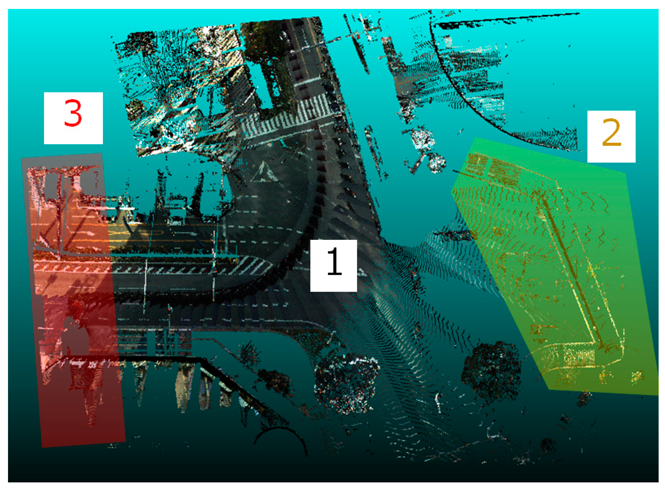
Figure 7.
Elevation view of measurement range. (a) base data and sequential data (A); (b) sequential data (B).
Figure 7.
Elevation view of measurement range. (a) base data and sequential data (A); (b) sequential data (B).

Figure 8.
Location of road environment changes. (a) large-scale scenario (b) small-scale scenario.
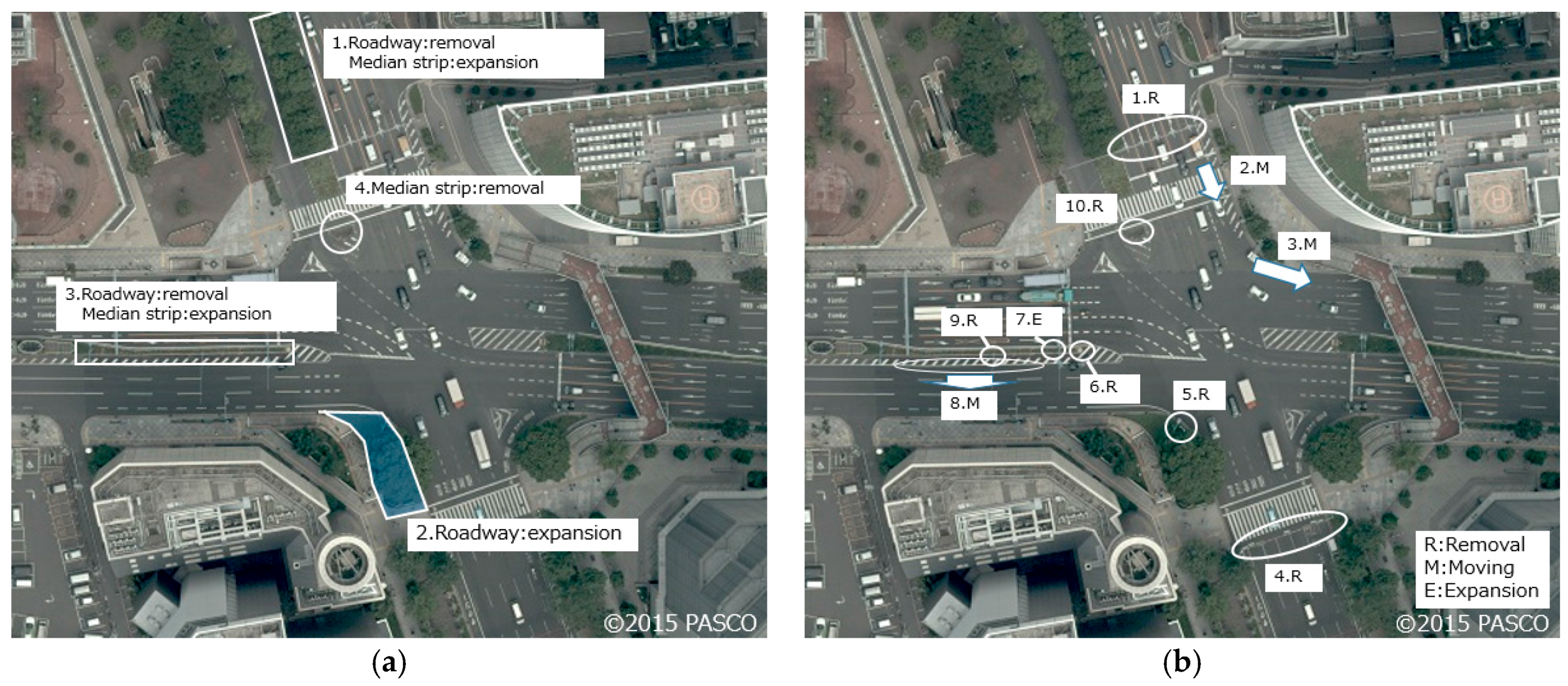
Figure 9.
Registration results.

Figure 10.
Results of measurement differences. (a) base data; (b) sequential data; (c) results.

Figure 11.
Results for large-scale changes before the correcting process.

Figure 12.
Results for large-scale changes after the correcting process.

Figure 13.
Errors after applying registration. The red area pointed by the arrow is the incorrect detection.
Figure 13.
Errors after applying registration. The red area pointed by the arrow is the incorrect detection.

Table 1.
Data for 3D road maps.
| Type of Data | Application | Advantage | Disadvantage |
|---|---|---|---|
| Base data | Map building | High accuracy | High cost |
| High density | Less frequent | ||
| Sequential data | Change detection | Low cost | Low accuracy |
| More frequent | Low density |
Table 2.
The specification of sequential data.
| Data | Positioning Error (X,Y,Z) (Meter) | Angle Error (Roll, Pitch, Yaw) (Degree) | Point Density (MMS = 1) | Measurement Range | Ratio in All Data |
|---|---|---|---|---|---|
| (A) | (5,5,5) | (0.1, 0.05, 0.05) | Wide | Low (33%) | |
| (B) | (10,10,10) | (0.1, 0.1, 0.1) | Narrow | High (67%) |
Table 3.
Contents of road environment changes.
| Scenario | Number in Figure 8 | Object | Change | Scenario | Number in Figure 8 | Object | Change |
|---|---|---|---|---|---|---|---|
| Large | 1 | Roadway | Removal | Small | 4 | Signboard | Removal |
| Large | 2 | Roadway | Expansion | Small | 5 | Lamppost | Removal |
| Large | 3 | Roadway | Removal | Small | 6 | Flasher | Removal |
| Large | 4 | Median strip | Removal | Small | 7 | Lamppost | Expansion |
| Small | 1 | Signboard | Removal | Small | 8 | Rubber pole | Moving |
| Small | 2 | Traffic signal | Moving | Small | 9 | Traffic enforcement camera | Removal |
| Small | 3 | Traffic enforcement camera | Moving | Small | 10 | Short pole | Removal |
Table 4.
Prepared data in the experiment. Performance: (A) is higher than (B) among sequential data Recorded change: T: Tentative change, RE: Road Environment change.
Table 4.
Prepared data in the experiment. Performance: (A) is higher than (B) among sequential data Recorded change: T: Tentative change, RE: Road Environment change.
| Sequential # | 1 | 2 | 3 | 4 | 5 | 6 | 7 | 8 | 9 |
|---|---|---|---|---|---|---|---|---|---|
| Performance | (A) | (B) | (B) | (A) | (B) | (B) | (B) | (A) | (B) |
| Recorded change | T | T | T | T | T | T·RE | T·RE | T·RE | T·RE |
Table 5.
Correct classification rate of tentative changes. The number in parenthesis is percentage of correct identifications.
Table 5.
Correct classification rate of tentative changes. The number in parenthesis is percentage of correct identifications.
| Object | Change | Sequential Data Number | Total | ||
|---|---|---|---|---|---|
| 6 | 7 | 8 | |||
| Pedestrian | Addition | - | 3/4 (75) | - | 3/4 (75) |
| Removal | - | 3/3 (100) | 2/2 (100) | 5/5 (100) | |
| Vehicle | Addition | - | 2/2 (100) | - | 2/2 (100) |
| Removal | 4/4 (100) | - | 2/2 (100) | 6/6 (100) | |
| Shadow | Apparance | 1/2 (50) | 1/1 (100) | 1/1 (100) | 3/4 (75) |
| disappearance | - | 3/3 (100) | - | 3/3 (100) | |
Table 6.
Patterns of results in the small-scale change scenario.
| Road Environment (Before Change) | State in Base Data | Road Environment (After Change) | Pattern | Number of Changes |
|---|---|---|---|---|
| occupied | occupied | empty | (a) | 8 |
| unmeasured | (b) | 1 | ||
| empty | empty | occupied | (c) | 3 |
| unmeasured | occupied | (d) | 1 |
© 2017 by the authors. Licensee MDPI, Basel, Switzerland. This article is an open access article distributed under the terms and conditions of the Creative Commons Attribution (CC BY) license (http://creativecommons.org/licenses/by/4.0/).
Share and Cite
MDPI and ACS Style
Fuse, T.; Yokozawa, N. Development of a Change Detection Method with Low-Performance Point Cloud Data for Updating Three-Dimensional Road Maps. ISPRS Int. J. Geo-Inf. 2017, 6, 398. https://doi.org/10.3390/ijgi6120398
AMA Style
Fuse T, Yokozawa N. Development of a Change Detection Method with Low-Performance Point Cloud Data for Updating Three-Dimensional Road Maps. ISPRS International Journal of Geo-Information. 2017; 6(12):398. https://doi.org/10.3390/ijgi6120398
Chicago/Turabian StyleFuse, Takashi, and Naoto Yokozawa. 2017. "Development of a Change Detection Method with Low-Performance Point Cloud Data for Updating Three-Dimensional Road Maps" ISPRS International Journal of Geo-Information 6, no. 12: 398. https://doi.org/10.3390/ijgi6120398
Note that from the first issue of 2016, this journal uses article numbers instead of page numbers. See further details here.