A Double-Smoothing Algorithm for Integrating Satellite Precipitation Products in Areas with Sparsely Distributed In Situ Networks

Abstract

The spatial distribution of automatic weather stations in regions of western China (e.g., Tibet and southern Xingjiang) is relatively sparse. Due to the considerable spatial variability of precipitation, estimations of rainfall that are interpolated in these areas exhibit considerable uncertainty based on the current observational networks. In this paper, a new statistical method for estimating precipitation is introduced that integrates satellite products and in situ observation data. This method calculates the differences between raster data and point data based on the theory of data assimilation. In regions in which the spatial distribution of automatic weather stations is sparse, a nonparametric kernel-smoothing method is adopted to process the discontinuous data through correction and spatial interpolation. A comparative analysis of the fusion method based on the double-smoothing algorithm proposed here indicated that the method performed better than those used in previous studies based on the average deviation, root mean square error, and correlation coefficient values. Our results indicate that the proposed method is more rational and effective in terms of both the efficiency coefficient and the spatial distribution of the deviations.

1. Introduction

Precipitation is a major meteorological component with high variability. In hydro-meteorological research, precipitation estimation is a key reference parameter that provides valuable information for economic and social planning. This information can protect peoples’ lives and property. Traditional precipitation estimation is based on in situ observation data. The data collected using observational networks distributed in drainage basins are processed by applying a weighted average method [1], a smoothing or interpolation method [2], and/or a geographically tuned statistical method [3]. Such processes are used to obtain the initial values of many hydrological models. The temporal-spatial distribution of precipitation in Shaanxi Province and northwestern China was studied using daily precipitation data from weather stations based on a linear regression analysis and the wavelet analysis method [4,5]. However, surface observational stations in China are mainly distributed in southeastern and central China, whereas the spatial distribution of stations in other regions is relatively sparse. Evaluation methods for ranking and ordering the daily rainstorms at each station were developed for this type of region by Cheng et al. [6]. Due to the obvious spatial variability of precipitation, the cumulative precipitation in each statistical area can vary considerably. Additionally, the precipitation distribution may be highly heterogeneous, and estimates of area rainfall that are interpolated have higher uncertainty than those determined using observational networks.

In recent years, scientists have made considerable efforts to use satellite images with global coverage for precipitation estimation. The Tropical Rainfall Measuring Mission (TRMM) is a joint project launched by the National Aeronautics and Space Administration (NASA) and the Japan Aerospace Exploration Agency (JAXA) in 1997 and provides abundant global tropical rainfall data [7,8,9]. In this paper, product 3B43 (version 7) of the real-time 3 h TRMM Multi-satellite Precipitation Analysis (TMPA) was selected as the object of the experiment. TMPA has been directly applied in various hydro-meteorological studies [10,11]. However, the spatial resolution of TMPA is less than satisfactory for studies involving meteorological or hydrological heterogeneity [12]. The low resolution of satellite-based estimation restricts its hydro-meteorological application. Nevertheless, because of its time delay, high-quality temporal sampling, and wide global coverage, TMPA provides valuable data for use in such applications. The fusion of TMPA and surface observation data has at least two advantages: (i) the errors of the two types of rainfall estimations are independent and (ii) in areas where surface observation stations are sparsely distributed, rainfall distributions constructed by TMPA can be an important reference.

By the end of the 20th century, the spatial statistics method had been introduced into precipitation estimation algorithms, enabling the combination of satellite and surface observations. However, this approach is subject to on-going improvement. Plouffe et al. [13] compared four spatial interpolation techniques: inverse distance weighting, thin-plate splines, ordinary kriging, and Bayesian kriging. Their results indicated that Bayesian kriging performed best for low rainfall in Sri Lanka. Zhang et al. [14] presented a method to estimate areal mean rainfall (AMR) using the Biased Sentinel Hospital-Based Area Disease Estimation (B-SHADE) model, biased rain gauge observations, and TRMM data in remote areas with sparse and uneven distributions of rain gauges. The results indicated that B-SHADE exhibited the lowest estimation biases. Chee et al. [15] considered nonparametric estimation of a mixing distribution by minimizing the quadratic distance between the empirical distribution and the mixture distribution, both of which were smoothed using kernel functions. Experimental studies showed that the new mixture-based density estimators outperformed the popular kernel-based density estimators in terms of mean integrated squared error for practically all the distributions studied as a result of the substantial bias reduction provided by nonparametric mixture models and double smoothing. Shao et al. [16] presented a double-smoothing technique to derive the precipitation amounts at a small grid size based on gauge observations. They used an empirical transformation to stabilize the residuals and could easily upscale the precipitation using the bootstrapping method.

The objective of the study by Long et al. [17] was to present a satellite and rain gauge data-merging framework adapted for coarse-resolution and data-sparse designs. In the framework, a statistical spatial downscaling method based on the relationships between precipitation, topographical features, and weather conditions was used to downscale the 0.25 daily rainfall field derived from the TMPA precipitation product. The nonparametric merging technique of double kernel smoothing, which was adapted for the data-sparse design, was combined with the global optimization method of shuffled complex evolution to merge the downscaled TRMM and gauged rainfall with minimum cross-validation error. Nerini et al. [18] compared two nonparametric rainfall data-merging methods with two geostatistical methods to optimize the hydrometeorological performance of a satellite-based precipitation product over a mesoscale tropical Andean watershed in Peru. The results were assessed using the following methods: (1) a cross-validation procedure and (2) a catchment water balance analysis and hydrological modelling. They found that the double-kernel smoothing method delivered the most consistent improvement over the original satellite product in both the cross-validation and hydrological evaluation. Thus, a systematic approach to the selection of a technique for merging satellite-rain gauge data based on the data characteristics was proposed.

Subdaily satellite-based rainfall data were analysed by Pfeifroth et al. [19] in West Africa, a region with considerable diurnal variability. Ingebrigtsen et al. [20] investigated aspects of various estimates using a Bayesian non-stationary spatial model of annual precipitation based on observations from multiple years. The model contained replicates of spatial fields, which increased the precision of estimates and made them less sensitive to prior values. They analysed precipitation data from southern Norway and investigated the statistical properties of the replicate model in a simulation study. A study in Australia [21] evaluated selected geostatistical methods for estimating daily rainfall maps across Australia. This study examined the changes in the support problem and spatial intermittency of daily rainfall data by blending satellite and gauge data. A geographically weighted regression (GWR) [22] was used to estimate the spatial distribution of the TRMM product error using elevation and geographical latitude and longitude as independent variables. A rainfall model was developed by combining ground-based and satellite-based rainfall measurements, and the model precision was validated using a cross-validation method based on rainfall gauge measurements. Study results from China [23] showed that compared to TMPA, Integrated Multisatellite Retrievals for the Global Precipitation Measurement (GPM), referred to as IMERG, significantly improved the estimation accuracy of precipitation in the Xinjiang region and on the Qinghai-Tibetan Plateau. However, most IMERG products over these areas are unreliable.

Gotway et al. [24] provided an up-to-date overview of how to solve the problem of incompatible spatial data. Kyriakidis [25] presented a geo-statistical method based on variations in the spatial resolution, in which suitable area-to-area and area-to-point covariance structure models are adopted to calculate and obtain area data and for prediction at a desired point. Pan et al. [26] and Gao et al. [27] adopted the optimum interpolation method for a fusion test based on satellite and surface observation data and reached similar conclusions, namely, that the fused product appreciably improved the precision of precipitation estimation and expanded the scope of estimation to reflect precipitation information for platforms at various scales. Shen et al. [28] evaluated the quality of the fused product and found indications that the fused product became more rational in terms of both precipitation value and spatial distribution by effectively utilizing the respective advantages of surface observations and satellite-retrieved precipitation. This fusion method reduced the average deviation and root-mean-square error, and it further improved product quality and presented a certain advantage in quantitatively monitoring heavy precipitation. The present paper proposes a new statistical method that fuses TMPA and surface observation data. When there are TMPA data deviations and no relatively strong spatial hypothesis, this method can still generate an extremely satisfactory nonparametric statistical framework and achieve excellent intermittent correction and spatial interpolation, even in areas in which surface observation stations are sparsely distributed.

2. Study Area and Experimental Data

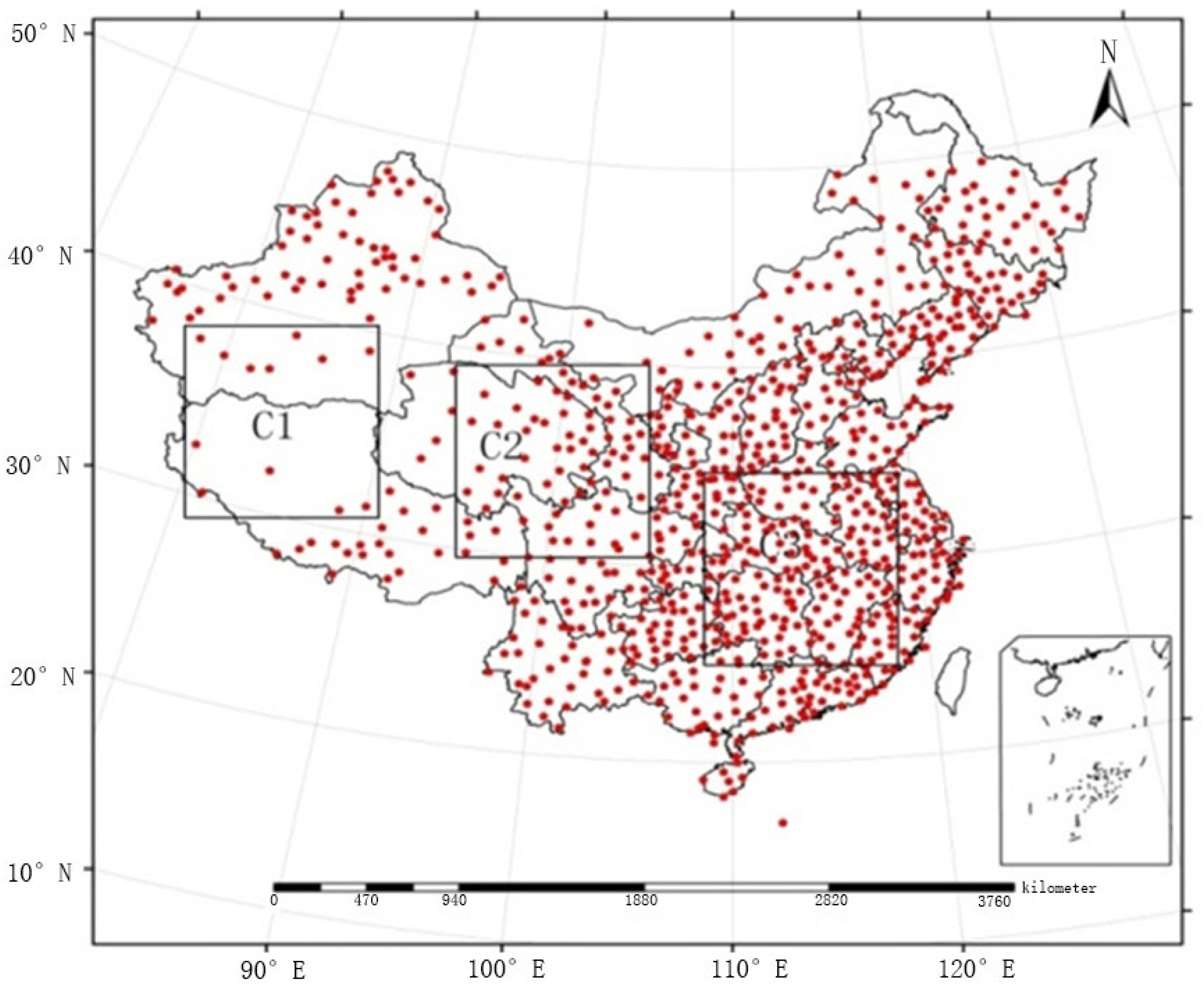
In this paper, the automatic weather station data were derived from the China Meteorological Data Sharing Service System Network, and they were prepared in daily value data files by the National Meteorological Information Center (NMIC). This network includes 839 stations covering the time interval from 2005 to 2010. Due to the complex topography of China, the spatial distribution of the national network of pluviometers in automatic weather stations is uneven (i.e., it is dense in the east and sparse in the west). Thus, it is necessary to evaluate the quality of the fusion method in regions with different densities. Three equal sizes of grid regions were selected according to the experimental area, i.e., region C1 in the west (where there are 12 mostly sparsely distributed stations), region C2 in the centre (where there are 68 stations), and region C3 in the southeast (where there are 162 more densely distributed stations), as shown in Figure 1. The automatic weather station data in C1, C2, and C3 were fused with the TMPA precipitation product, and their results were labelled as “C1”, “C2”, and “C3”, respectively. The fusion effects under the three regional network densities were tested.

TMPA, the seventh-edition product of TRMM adopted for satellite data, has been recognized as the product with the highest precision among the TRMM precipitation products. The precipitation analysis data obtained per 3 h by TMPA were first accumulated into daily precipitation data and then into monthly precipitation data. The TMPA precipitation product adopted in this paper ranged from 2005 to 2010 in terms of time interval and from 10° N to 50° N latitude.

3. Method for Integrating Satellite Precipitation Products

The method proposed in this paper is used to estimate precipitation by fusing various spatial data, and it is derived from the theory of data assimilation. Data assimilation involves the processing of different sources of data so that the final products can be integrated. In numerical weather prediction, data assimilation is initially considered a process used to provide initial fields for the numerical prediction of the spatial and temporal distributions of observation data. The key to this method lies in calculating the differences between area data and point data. The interpolation method adopted in this paper is kernel smoothing, which, in contrast to the Kriging method, does not depend on the stationarity hypothesis and can be applied in circumstances in which the geographical statistical hypothesis has failed, i.e., when the geographic data involved in a statistical analysis of geography are related or correlated, heterogeneous, and do not meet the randomness assumptions of the general statistical analysis. Moreover, two issues related to the residual error-based fusion method are discussed: (1) employing the original TMPA as the background field is problematic; thus, the pre-processing of area data is essential; (2) the ordinary kernel smoothing method, after being improved, can improve visual expression and the efficiency of estimation in a sparse area.

3.1. Principle of Residual Error-Based Nonparametric Data Fusion

While the key to residual error-based analysis lies in calculating the differences between the background field and the observed values, the residual error-based nonparametric fusion method aims to solve the weighted average of residual errors according to the distance between observation points. The estimation field is obtained through combining the residual error field with the background field. Therefore, the estimation field is obtained through the adjustment of adjacent observation data, and the background field will be retained if there are no local observation data.

The relationships among the background field X_B, the observation field X_O, and the residual error D can be expressed by the following system of equations:

$$X_B=X_T+e_B$$

(1)

$$X_O=X_T+e_O$$

(2)

$$D=X_B-X_O$$

(3)

where e_B and e_O represent the background error and the observation error, respectively, and X_T represents the real field. It is assumed that X_B is known at any point of S, which is a 2-dimensional point set, whereas X_O can be solved at the observation points.

$$S_{\mathrm{i}}\in S, \mathrm{i}=1,\dots ,N$$

(4)

where N is the number of observation points.

It is also assumed that the background error e_B meets the conditions

$$E\left({\mathrm{e}}_B\right)={\mu }_B$$

(5)

and

$$V\mathrm{ar}\left({\mathrm{e}}_B\right)={{\displaystyle \sigma }}_B^2$$

(6)

where μ_B cannot be 0 and will vary in space.

Although independent assumptions exist, the background error of two adjacent pixels of the raster data is generally related. In comparison to the model in which the correlated error is more accurate, the violation of the independence assumption can lead to a larger estimation variance. However, the deviation is still close to zero. If there is a strong correlation, it is more difficult to obtain estimates of uncertainty. This case is not considered in this study. In future studies, this independence assumption will take into account the background error and the computation of uncertainty.

In contrast with the background error, the measurement error is considered as white Gaussian noise and is expressed as

$$E\left({\mathrm{e}}_{\mathrm{O}}\right)=0$$

(7)

and

$$V\mathrm{ar}\left({\mathrm{e}}_{\mathrm{O}}\right)={{\displaystyle \sigma }}_{\mathrm{O}}^2$$

(8)

White Gaussian noise is a type of accidental error that follows the normal distribution. Accidental error is the error caused by the uncertainty of the measurement, including human error.

According to Equations (1)–(3), the nonparametric model is used to express the residual error field, as shown by the formula below:

$$D\left(S_{\mathrm{i}}\right)=e_B\left(S_{\mathrm{i}}\right)-e_O\left(S_i\right)$$

(9)

Equation (9) indicates that the residual error field is equal to the difference between the background error and the observation error. The estimation field X_M can adopt the residual error-based nonparametric model for estimation, as shown by the formula below:

$$D\left(S_{\mathrm{i}}\right)=X_B\left(S_{\mathrm{i}}\right)-X_O\left(S_i\right)$$

(10)

$${\stackrel{\wedge }{\mu }}_B\left(S\right)=\{\begin{array}{l}\frac{{\displaystyle {\sum }_{i=1}^{n}K\left(\Vert S-S_i\Vert /h\right)D\left(S_i\right)}}{{\displaystyle {\sum }_{i=1}^{n}K\left(\Vert S-S_i\Vert /h\right)}}\\ 0\end{array} if {\displaystyle {\sum }_{i=1}^{n}K\left(\Vert S-S_i\Vert /h\right)>0}$$

(11)

Otherwise,

$$X_M\left(S\right)=X_B\left(S\right)-{\stackrel{\wedge }{\mu }}_B\left(S\right)$$

(12)

where ||...|| is the measured distance. The kernel function meets the three conditions

$$K\left(\mathrm{u}\right)\ge 0$$

(13)

$$K\left(\mathrm{u}\right)=K\left(-\mathrm{u}\right)$$

(14)

$${\displaystyle \int K\left(\mathrm{u}\right)} \mathrm{du}=1$$

(15)

where h is a positive number and is referred to as the bandwidth. The nonparametric model employs the kernel function to assign the weights according to the distances between peripheral observation points.

The adoption of the residual error-based nonparametric fusion method involves three steps: (i) calculate the residual error at the observation point using Equation (10); (ii) adopt the kernel-smoothing method to estimate the background error generated by the residual error using Equations (20) and (21); and (iii) extract the estimation field or the effective background field according to the estimated background error using Equation (12).

3.2. Setting the Background Field

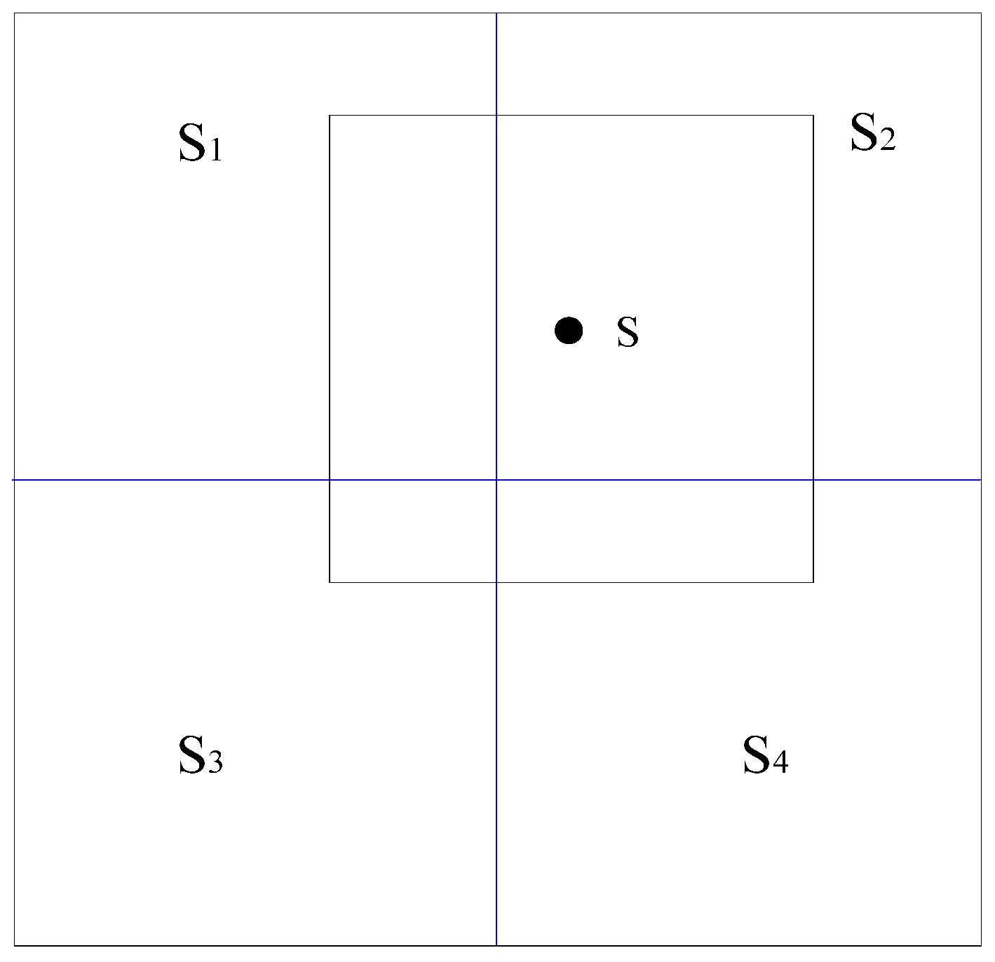
The method described in this paper is given by Equations (10)–(12) and aims to fuse raster data and point data. Thus, clearly defining the background field is essential. Given that “direct fusion” [29] generates significant deviations on the plane boundary (i.e., the boundary between two continuous TMPA raster datasets) and causes discontinuity in the background field, this paper introduces the “smoothing fusion” method to reduce the boundary deviations caused by the fusion of raster data and point data. The basic idea of the method is to employ the moving average of TMPA to generate a smoothing field and adopt the auxiliary field as the background field of Equations (10)–(12). The window used by the moving average has the same size as that of a pixel in the TMPA raster dataset. S_i (i = 1, 2, 3, 4) represents four TMPA raster pixels containing the moving average s; A_i (i = 1, 2, 3, 4) represents the area of intersection between S_i and the moving window, as shown in Figure 2.

Moreover, T(s_j) represents the TMPA precipitation estimation for raster S_i. The smoothed TMPA at s is provided by the formulas [30] below:

$$T^{\ast }\left(\mathrm{s}\right)={\displaystyle \sum _{j=1}^4{w}_{j}T\left({\mathrm{s}}_j\right)}$$

(16)

$$w_j=A_j/{\displaystyle \sum _{i=1}^n{A}_i}$$

(17)

3.3. Double-Smoothing Algorithm

Kernel smoothing (Equation (11)) can be employed to effectively estimate the expectations of the background error field, and its conditions meet the residual error field under circumstances where observation points are densely distributed. However, the performance of ordinary kernel smoothing is not stable enough, especially because it cannot reflect real expectations well when the observation points are sparsely distributed. More accurately, the conditional mean of background errors is solved by using Equation (11), i.e.,

$${\displaystyle {\sum }_{i=1}^{n}K\left(\Vert S-S_i\Vert /h\right)}$$

(18)

from which it can be seen that

$${\displaystyle {\sum }_{i=1}^{n}K\left(\Vert S-S_i\Vert /h\right)>0}$$

(19)

if and only if there is at least one S_i located in the bandwidth radius h of S. Assuming that only one observation point falls within the scope of the samples, the estimated background error outside of the observed bandwidth radius will be zero, but it will be significantly different within the observed bandwidth radius, resulting in discontinuity of the precipitation estimation. In remote regions of China, the spatial distribution of the pluviometers of automatic weather stations is extremely sparse, and there are no automatic weather stations in many regions. Thus, having adopted the double-smoothing technique [31], this study indicated that the double-smoothing estimation was smooth on the surfaces of all regions, which ensured that the background field estimation was smooth enough and could meet the smoothness hypothesis of the basic background field. Subsequently, the fusion method of Equation (11) was referred to as single smoothing.

Double-smoothing estimation is based on the following process: first, new pseudo-observation data are added through rough interpolation; second, the estimated value is obtained from the pseudo-observation data, which were obtained through interpolation, and the original data. Thus, the double-smoothing estimation can be divided into two steps [30].

(1) Convert the original data D(si) into the rasterized pseudo-data with raster size L.

$$\stackrel{\wedge }{D}\left(s_k^{\ast }\right)=\frac{{\displaystyle {\sum }_{i=1}^n{K}_1\left(\Vert s_k^{\ast }-s_i\Vert /h_1\right)D\left(s_i\right)}}{{\displaystyle {\sum }_{i=1}^n{K}_1\left(\Vert s_k^{\ast }-s_i\Vert /h_1\right)}}$$

(20)

(2) Estimate the background error field from the extended dataset, including original data and pseudo-data.

$${\stackrel{\wedge }{\mu }}_B^D\left(s\right)=\frac{{\displaystyle {\sum }_{i=1}^n{K}_2\left(\Vert s-s_i\Vert /h_2\right)D\left(s_i\right)+}{\displaystyle {\sum }_{\mathrm{k}=1}^{\mathrm{K}}{K}_2\left(\Vert s-s_{\mathrm{k}}^{\ast }\Vert /h_2\right)\stackrel{\wedge }{D}\left(s_{\mathrm{k}}^{\ast }\right)}}{{\displaystyle {\sum }_{i=1}^n{K}_2\left(\Vert s-s_i\Vert /h_2\right)+}{\displaystyle {\sum }_{\mathrm{k}=1}^{\mathrm{K}}{K}_2\left(\Vert s-s_{\mathrm{k}}^{\ast }\Vert /h_2\right)}}$$

(21)

As an empirical value, the bandwidth h₁ was set at h₁ = 0.3 in this paper; the bandwidth h₂ was determined through cross-validation. K is the amount of pseudo-data. The kernel function K₁ adopted a Gaussian kernel function, and the kernel function K₂ adopted the Epanechnikov kernel. To ensure the sufficiency of extended data, the raster size L of pseudo-data must meet the condition αL < h₂, where α > 1. According to Goudenhoofd et al. [29], the parameter α was set to 1.2, and the minimum value of h₂ was 0.3. The raster size L of the generated pseudo-data was 0.25°, which is equal to the resolution of TMPA.

3.4. Fusion Method of Precipitation Estimation

First, the TMPA data are produced by smoothing the precipitation data adopted for satellite TRMM 3B43 using Equations (1) and (2). Second, the residual error field D(si) is generated by subtracting the pluviometer observation data based on the TMPA data using Equation (10). Third, the pseudo-data are calculated based on the residual error field using Equation (20); then, the data set is expanded according to the residual error field and the pseudo-data, and the background error field is generated using Equation (21). Finally, the estimation field X_M(Si) is formed by subtracting the background error field from the background field using Equation (12). This process is shown in Figure 3.

4. Experimental Results

The average deviations (AD), root-mean-square errors (RMSE), and correlation coefficients (CC) of the fusion method under the three different regional network densities in China for July 2009 are provided in

Table 1. Average deviations (AD), root-mean-square errors (RMSE), and correlation coefficients (CC) of the fusion methods under the three different regional network densities in China in July 2009. FMS, the fusion method proposed by Shen et al. ([28]), FMP, the fusion method proposed in this paper.

Region	FMS			FMP
	AD (mm/h)	RMSE (mm/h)	CC	AD (mm/h)	RMSE (mm/h)	CC
C1	−0.121	2.328	0.309	−0.082	1.960	0.455
C2	−0.060	1.876	0.732	−0.058	1.833	0.701
C3	−0.024	1.747	0.798	−0.037	1.808	0.722

.

$$AD=\frac{{{\displaystyle \sum }}_{\mathrm{i}=1}^{\mathrm{N}}\{{\mathrm{X}}_{\mathrm{M}}\left({\mathrm{s}}_{\mathrm{i}}\right)-{\mathrm{X}}_{\mathrm{o}}\left({\mathrm{s}}_{\mathrm{i}}\right)\}}{\mathrm{N}}$$

(22)

$$\mathrm{RMSE}=\sqrt{\frac{{{\displaystyle \sum }}_{\mathrm{i}=1}^{\mathrm{N}}{\{{\mathrm{X}}_{\mathrm{M}}\left({\mathrm{s}}_{\mathrm{i}}\right)-{\mathrm{X}}_{\mathrm{o}}\left({\mathrm{s}}_{\mathrm{i}}\right)\}}^2}{\mathrm{N}}}$$

(23)

$$\mathrm{CC}=\frac{{{\displaystyle \sum }}_{\mathrm{i}=1}^{\mathrm{N}}\{{\mathrm{X}}_{\mathrm{M}}\left({\mathrm{s}}_{\mathrm{i}}\right)-\overline{{\mathrm{X}}_{\mathrm{M}}}\}\{{\mathrm{X}}_{\mathrm{o}}\left({\mathrm{s}}_{\mathrm{i}}\right)-\overline{{\mathrm{X}}_{\mathrm{O}}}\}}{\sqrt{{{\displaystyle \sum }}_{\mathrm{i}=1}^{\mathrm{N}}{\{{\mathrm{X}}_{\mathrm{M}}\left({\mathrm{s}}_{\mathrm{i}}\right)-\overline{{\mathrm{X}}_{\mathrm{M}}}\}}^2{{\displaystyle \sum }}_{\mathrm{i}=1}^{\mathrm{N}}{\{{\mathrm{X}}_{\mathrm{O}}\left({\mathrm{s}}_{\mathrm{i}}\right)-\overline{{\mathrm{X}}_{\mathrm{O}}}\}}^2}}$$

(24)

With an increasing distribution density of pluviometers, the average deviations and root-mean-square errors of the two fusion products decreased, which was accompanied by an increased spatial correlation.

In region C1, where pluviometers are sparsely distributed, the fusion method proposed in this paper (referred to as FMP) yielded an average deviation of −0.082 mm/h, a root-mean-square error of 1.960 mm/h, and a correlation coefficient of 0.455. In region C2, where pluviometers are moderately distributed, the estimation error was reduced; the average deviation and root-mean-square error were reduced to −0.058 mm/h and 1.833 mm/h, respectively, and the correlation coefficient was increased to 0.701. In region C3, where pluviometers are densely distributed, the average deviation and root-mean-square error were further reduced and the correlation coefficient reached as high as 0.722.

The fusion method proposed by Shen et al. [28] is referred to as FMS. In their paper, the merged precipitation product in China at an hourly, 0.1° latitude, and 0.1° longitude temporal-spatial resolution was developed through a two-step merging algorithm using a probability density function (PDF) and optimal interpolation (OI) based on the hourly precipitation observed at automatic weather stations in China and retrieved from CMORPH (Card programmed calculator MORPHing technique) satellite data.

Compared with FMS, FMP did not show any significant fluctuations in precipitation estimation and could realize a more stable overall estimation. In region C1, with the adoption of FMP, the average deviation was improved from −0.121 mm/h to −0.082 mm/h and the correlation coefficient was increased from 0.309 to 0.455, which suggests that it could greatly improve the precipitation estimation in regions in which pluviometers are sparsely distributed in China. In region C2, the two fusion methods were consistent in terms of precipitation estimation. In region C3, FMS was superior to FMP in terms of precipitation estimation, which suggested that it would be better to adopt FMS in regions where stations are densely distributed.

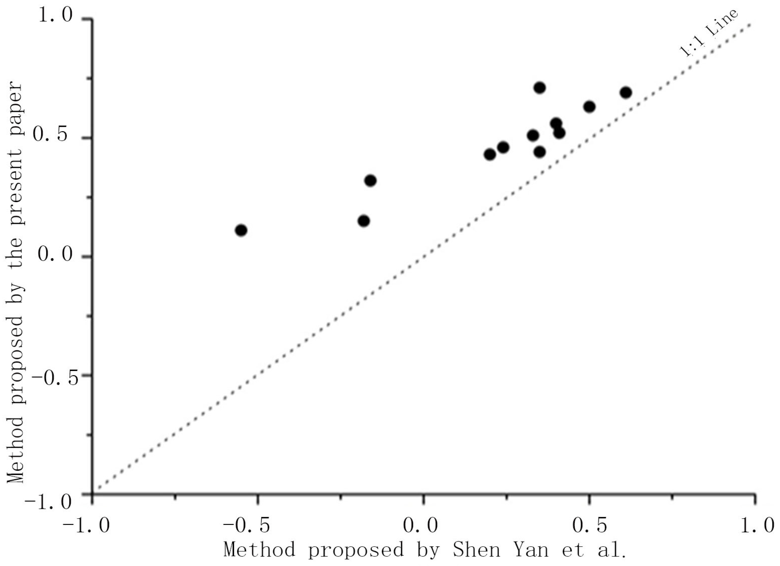
The coefficient of efficiency (CE) is the most common efficiency evaluation index in hydrological models; it is unitless and refers to the fraction of variance explained by a model.

$$CE=1-\frac{{{\displaystyle \sum }}_{\mathrm{i}=1}^{\mathrm{N}}\{{\mathrm{X}}_{\mathrm{M}}\left({\mathrm{s}}_{\mathrm{i}}\right)-{\mathrm{X}}_{\mathrm{o}}\left({\mathrm{s}}_{\mathrm{i}}\right)\}}{{{\displaystyle \sum }}_{\mathrm{i}=1}^{\mathrm{N}}{\{\overline{{\mathrm{X}}_{\mathrm{O}}}-{\mathrm{X}}_{\mathrm{O}}\left({\mathrm{s}}_{\mathrm{i}}\right)\}}^2}$$

(25)

This paper introduced CE to further experimentally compare the two fusion methods in terms of model efficiency in the sparsely distributed region C1. A comparison of the two fusion methods in terms of coefficient of efficiency in July 2009 is provided in Figure 4, which shows that all of the points (CE ratio value) were located above the line 1:1, suggesting that the method adopted by the y-axis was superior to that adopted by the x-axis. Thus, the test proved that it would be more effective to adopt FMP in sparsely distributed regions.

To more clearly demonstrate that FMP would be more accurate in regions in which pluviometers are sparsely distributed, this paper comparatively analysed the statistical indexes of the two fusion methods under various precipitation grades and tested the fusion results under these grades. According to the intensity of precipitation (IP), the hourly precipitation can be divided into five grades: <1.0 mm, 1.0–2.5 mm, 2.5–8.0 mm, 8.0–16.0 mm, and >16.0 mm.

Table 2. Statistical results of fusion under different grades of precipitation between May and September from 2005 to 2010. IP, intensity of precipitation.

IP (mm/h)	FMS			FMP
	AD (mm/h)	RD (%)	RMSE (mm/h)	AD (mm/h)	RD (%)	RMSE (mm/h)
<1.0	0.110	42.128	0.778	0.089	37.643	0.615
1.0–2.5	−0.044	−1.675	1.300	0.028	−0.876	1.021
2.5–8.0	−0.637	−13.747	2.398	−0.557	−9.402	1.950
8.0–16.0	−2.640	−23.906	4.898	−0.701	−11.853	2.456
≥16.0	−6.980	−30.967	9.960	−0.920	−14.461	3.937

shows that the average deviation and relative deviation (RD) of FMS vary from positive to negative. This variability suggests that low-level precipitation below 1.0 mm/h was overestimated, whereas precipitation of at least 1.0 mm/h was underestimated, and it shows that the deviation gradually increased with increasing intensity of precipitation. After the adoption of FMP, the precipitation field still showed deviations in precipitation estimates to some extent. However, the absolute values of the average deviation, relative deviation, and root-mean-square error under the same grade were significantly reduced in comparison to those under FMS. To be specific, after the adoption of FMP, the improvement in the results was most significant when the precipitation rate was above 8.0 mm/h. In particular, when the intensity of precipitation exceeded 16.0 mm/h, the relative deviation was reduced from the previous −30.967% to −14.461%. Thus, more accurate results could be achieved for a higher intensity of precipitation.

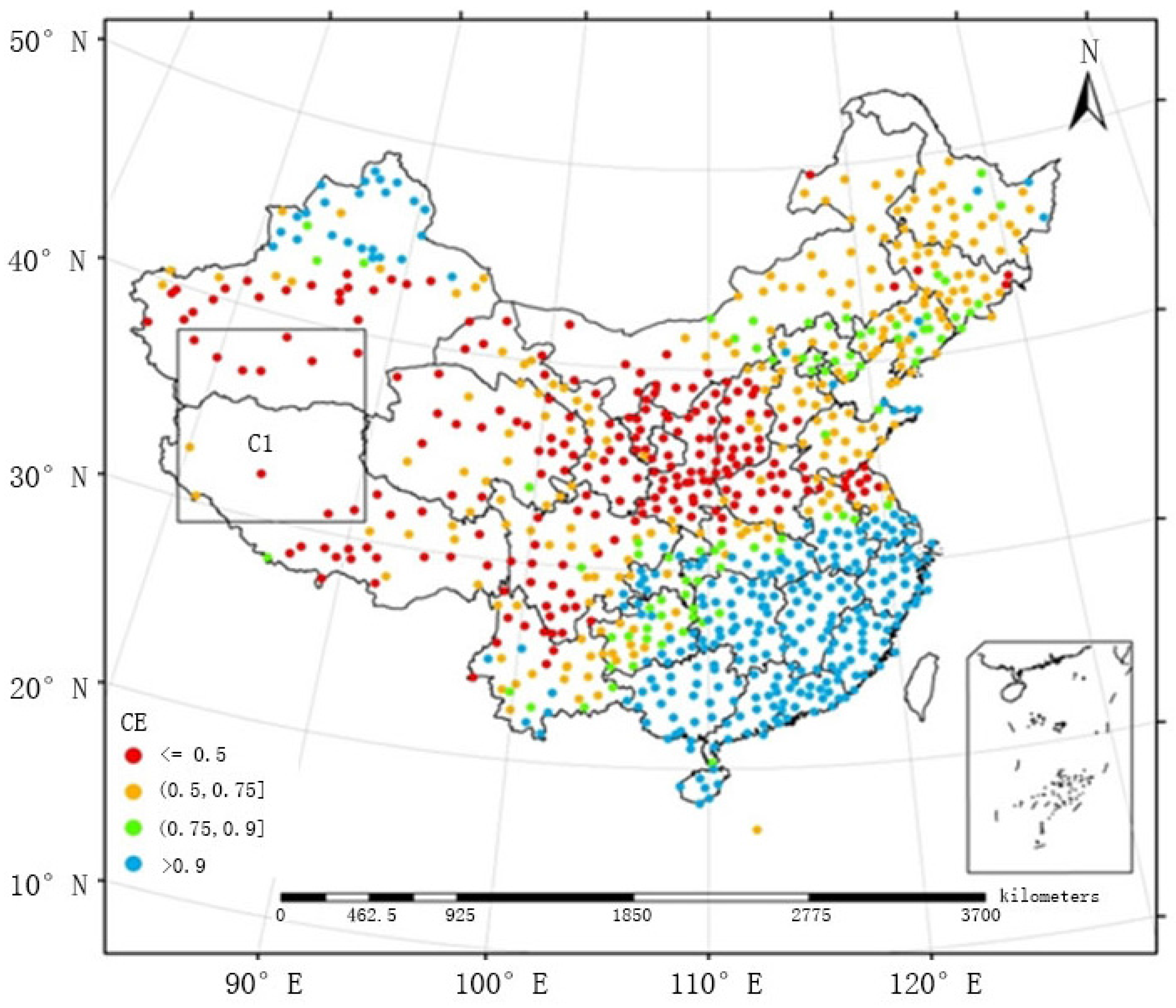
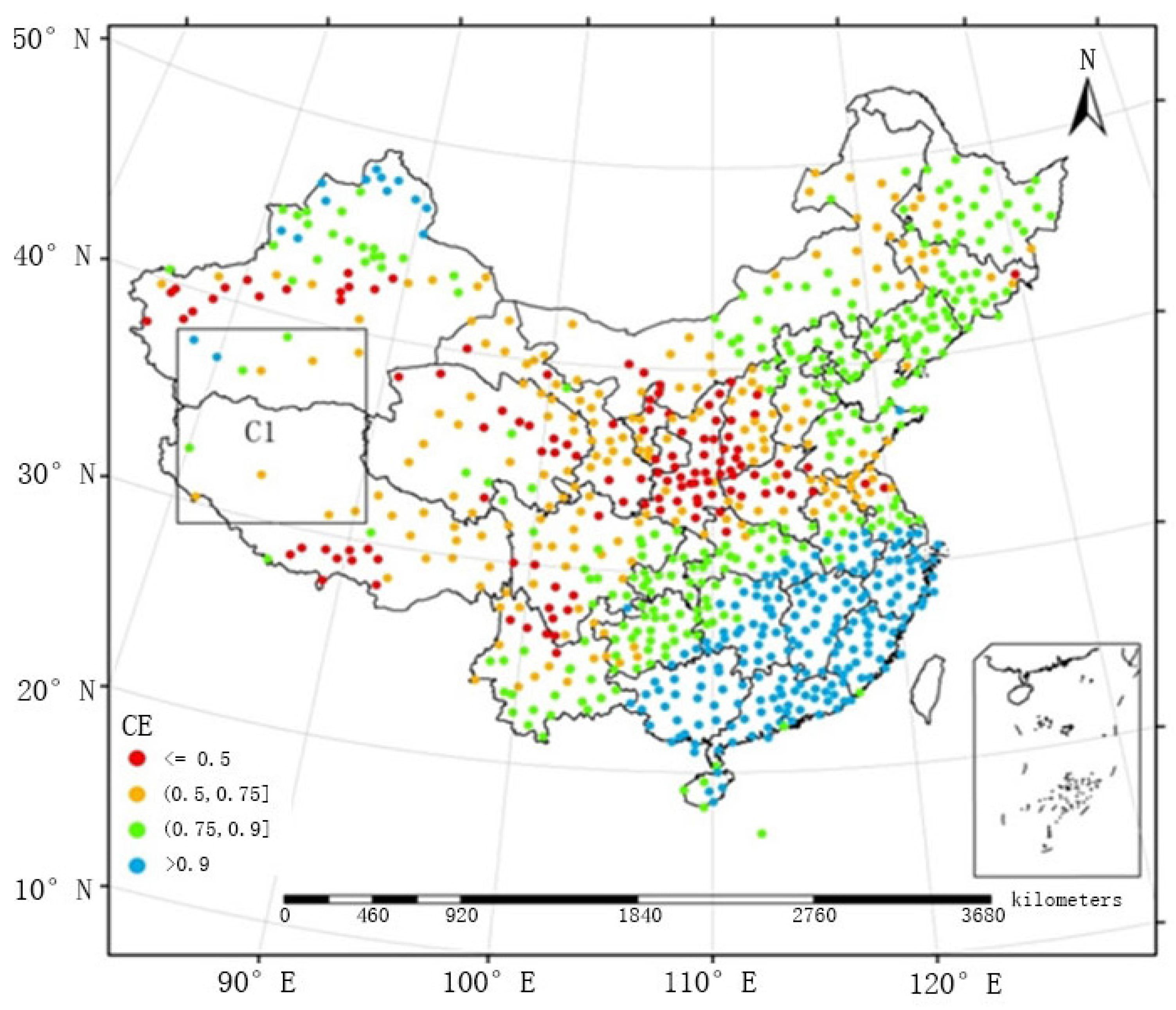
The following section discusses and compares the effectiveness of the models as a function of the spatial distribution of pluviometers. The spatial distributions of the coefficients of efficiency obtained by FMS and FMP between May and September from 2005 to 2010 are provided in Figure 5 and Figure 6, respectively. In some remote Chinese regions, the pluviometers are sparsely distributed (e.g., region C1 in Figure 5 and Figure 6), and FMS could not estimate the precipitation well; thus, the coefficients of efficiency were generally below 0.5. After the adoption of FMP, the coefficients of efficiency decreased within the range of 0.5 and 0.9 and even exceeded 0.9 in some cases, which demonstrated that it would be more accurate and effective to adopt FMP in regions in which pluviometers are sparsely distributed.

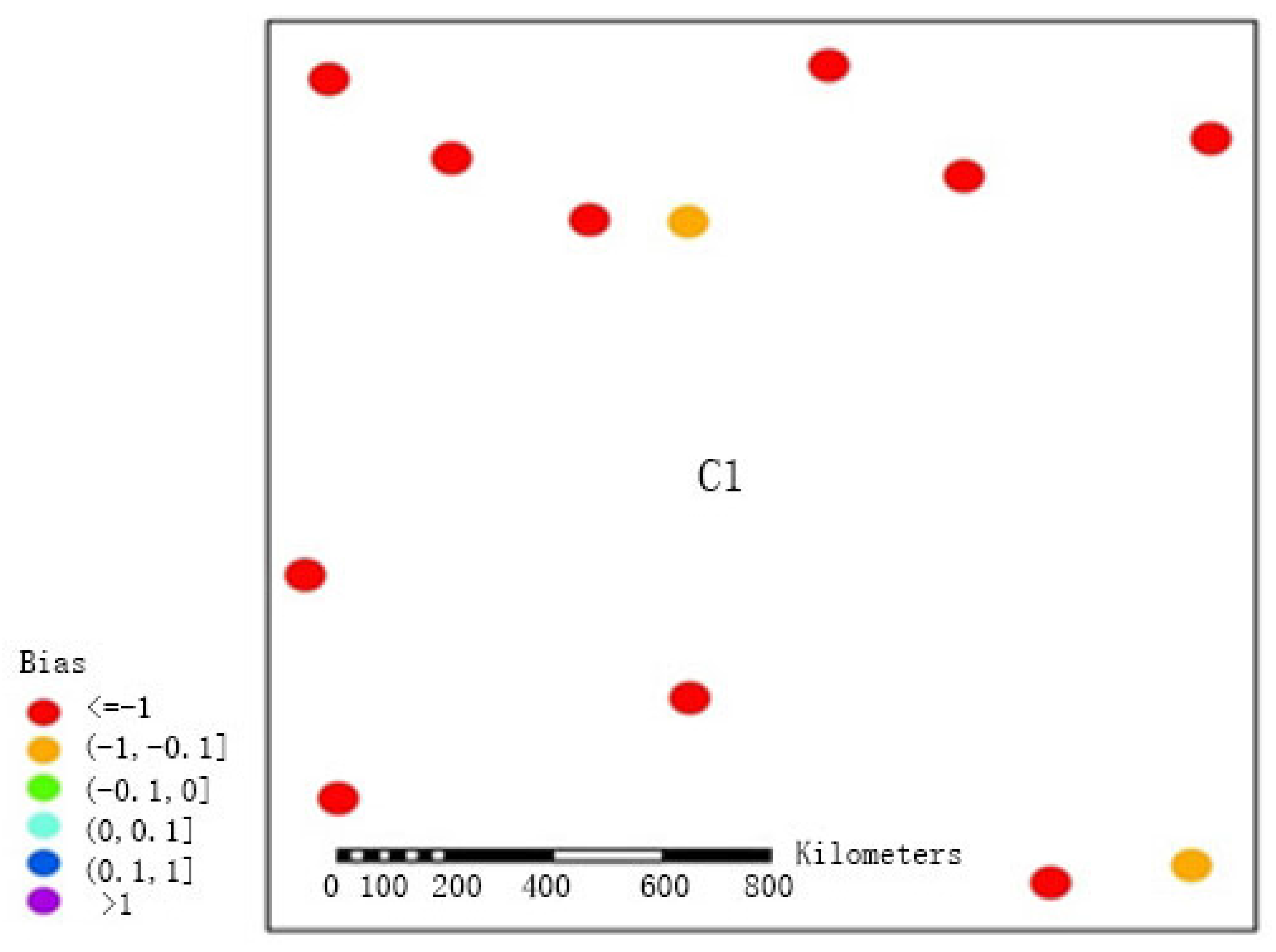
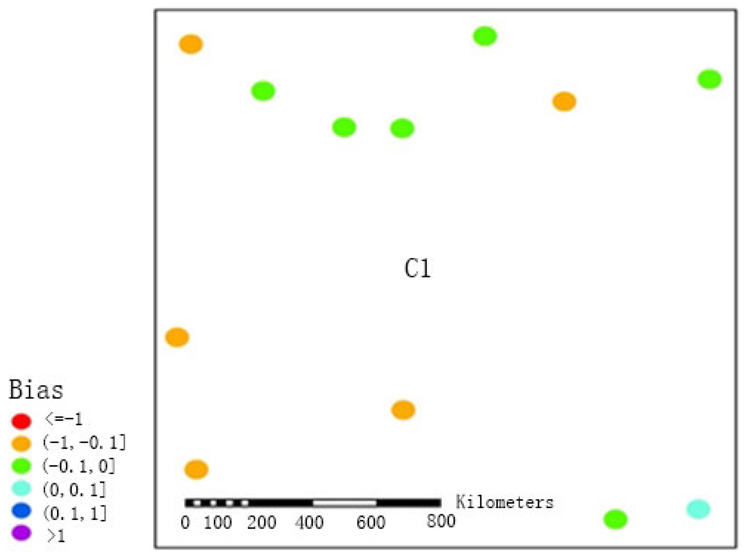
To further demonstrate that FMP would achieve more accurate results for precipitation estimation in regions in which pluviometers are sparsely distributed, we calculated the biases between the precipitation estimations obtained using the two methods and the precipitation observations obtained at the stations in region C1 between May and September from 2005 to 2010 (see the results in Figure 7 and Figure 8). Both methods underestimated precipitation in the sparsely distributed western region, which may be explained by the sparse distribution of pluviometers and by the local atmospheric convection; the biases obtained by FMS were mainly concentrated in the range of <−1, and the biases of only two stations ranged between −1 and −0.1. After the adoption of the double-smoothing algorithm of this paper for processing (FMP), the biases generally fell within the range of −1 to −0.1 (five stations) and the range of −0.1 to 0 (six stations), and only one station had a bias within the range of 0 to 0.1. This improvement fully demonstrated that in sparsely distributed regions, the double-smoothing algorithm could more effectively reduce errors and more satisfactorily reflect precipitation events.

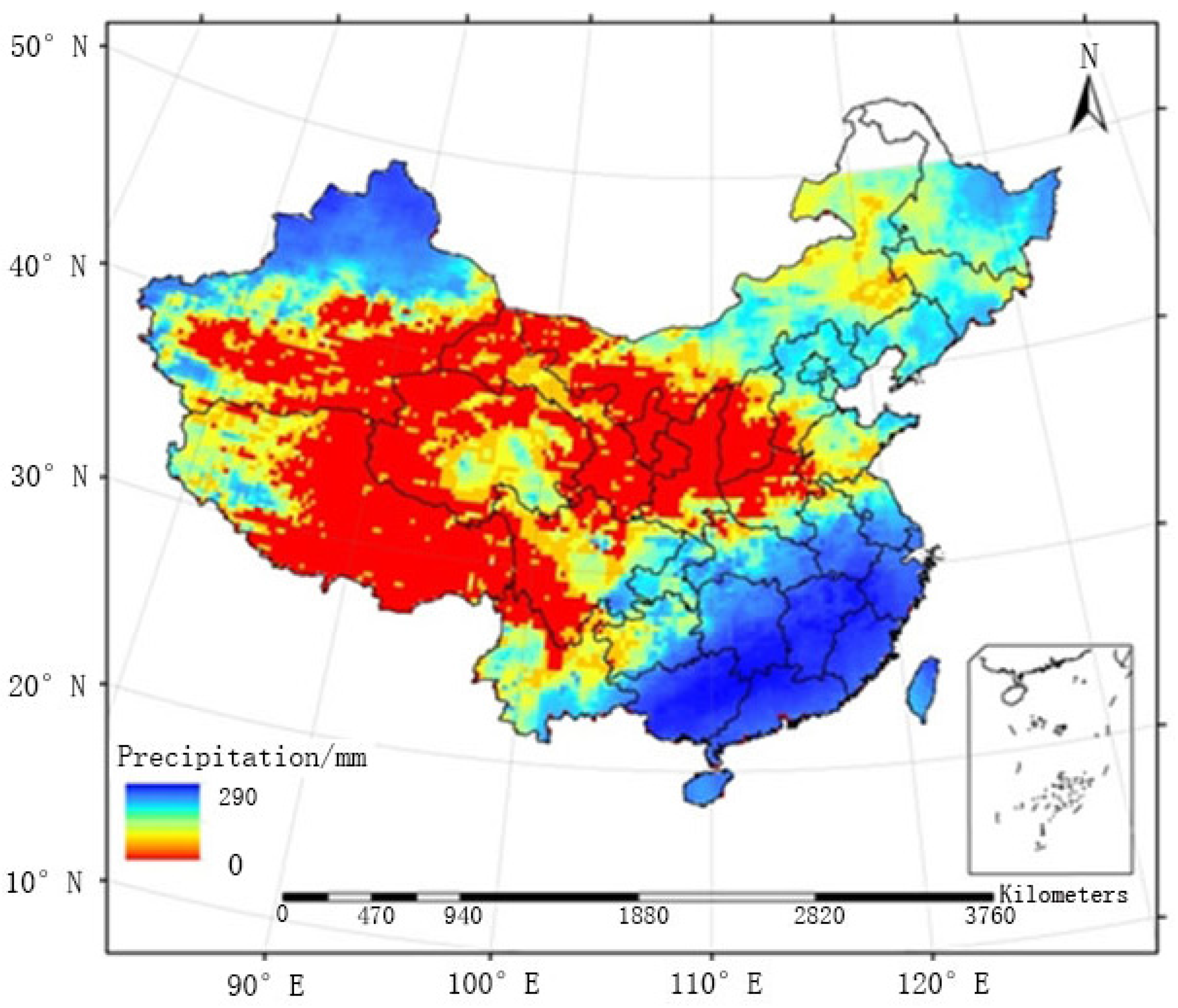
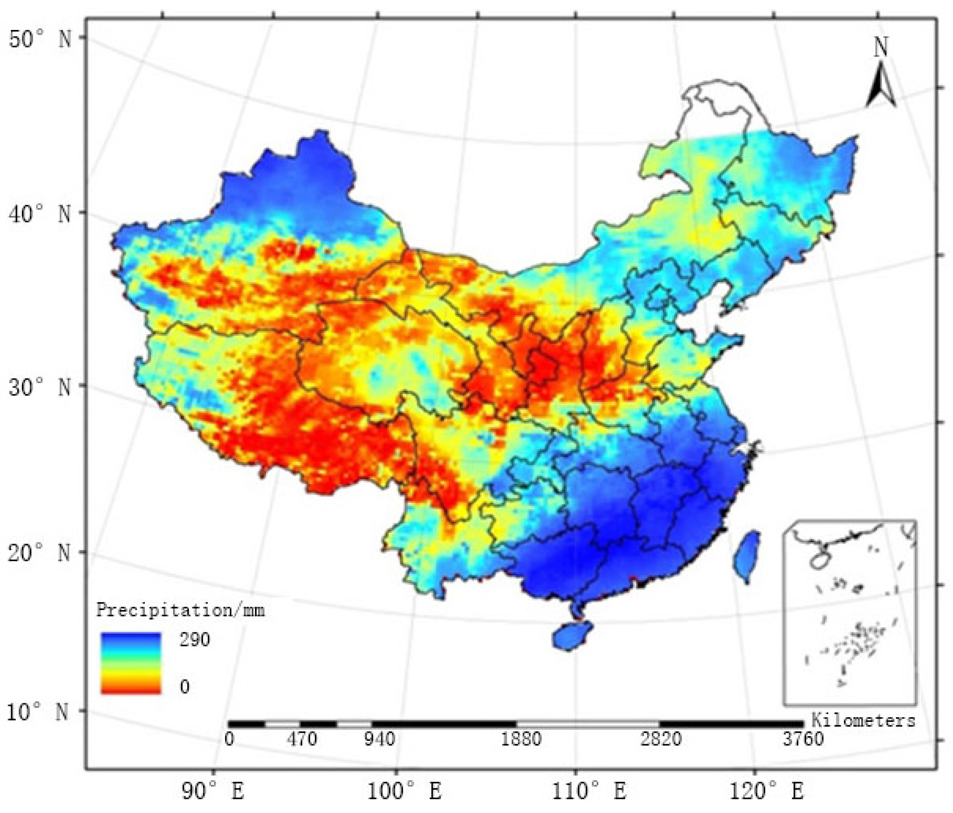
The raster map of the average monthly precipitation field generated by FMS and that generated by FMP between May and September from 2005 to 2010 are provided in Figure 9 and Figure 10, respectively. The two methods were similar in terms of the overall distribution of the precipitation field, and large precipitation events were mainly concentrated in the southeastern regions. The distribution of rainfall generated by FMS was relatively heterogeneous, especially in regions where surface observation stations are sparsely distributed (e.g., region C1). FMP, the method proposed in this paper, adopted a double-smoothing processing for sparsely distributed regions and improved the precision of the precipitation field, which is smoother, as shown below.

5. Conclusions

To address the issue of the sparse distribution of automatic weather stations in the western regions of China, the double-smoothing algorithm is adopted in this paper. The point data of precipitation, as observed by the pluviometers, and the raster data of precipitation from TMPA are integrated into a set of discrete points, transforming the two datasets into a new type of improved dataset. Additionally, the smoothing method is adopted to correct discontinuities before TMPA is fused. The experimental results indicate that compared with the method of Shen et al., the double-smoothing algorithm is more rational and effective in terms of both the magnitudes and spatial distribution of precipitation. That is, in regions in which pluviometers are sparsely distributed, the variation in the average deviation and root-mean-square error with time is insignificant. The double-smoothing algorithm can more accurately estimate heavy precipitation. The precipitation estimation method of this paper is proposed with a view towards individual differences; the next research objective is to introduce more variables into the background field to further improve the estimation efficiency.