
An Adaptive Agent-Based Model of Homing Pigeons: A Genetic Algorithm Approach


Abstract
:1. Introduction
Related Work
2. Materials and Methods
2.1. Data
2.2. The Model
2.2.1. Purpose
2.2.2. Entities, State Variables and Scales
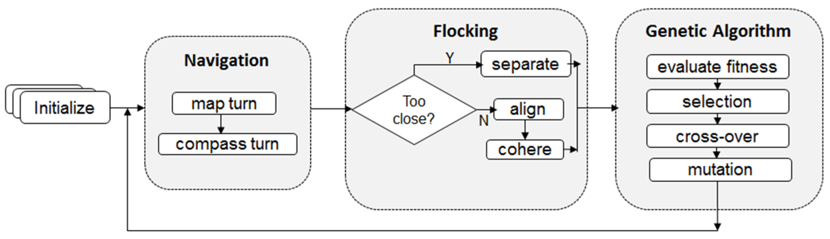
2.2.3. Process Overview and Scheduling
- State variables of pigeon agents are updated (or initialized if at the beginning of the model).
- Agents execute navigation decisions; specifically, “real” agents use values of relative turn angle (mean-turn) and step-distance which are attributes that are captured in the empirical GPS data streams to orient their heading by an angle equivalent to the mean-turn and to move forward by a distance equivalent to the step-distance. On the other hand, “simulated” agents choose their navigation behaviours on the basis of two sub-models, which are specified as map-turn and compass-turn. The aim of the map-turn parameter, alternatively referred to as the elevation-turn is to re-orient agent headings and allow agents to fly along a controlled topographic contour. On the other hand, compass-turn ensures that an agent dynamically maintains a general bearing towards a known home loft during navigation.
- Agents find flock mates with whom to navigate; flocking rules are adopted from Reynolds flocking model [67] and are guided by separation, alignment, and coherence procedures. These procedures are controlled by model parameters which are specified as minimum separation distance, maximum separation turn, maximum alignment turn, and maximum cohere turn. The separation procedure supersedes the other procedures under the flocking behaviour and by it, an agent changes its direction of flight to avoid colliding with nearby flock mates. An implementation of the flocking model is included as one of the library models within NetLogo package [68] and this is what we modified and adopted to fit the specifications and objectives of the model presented herein.
- Apart from the navigation and flocking behaviours, agents can also turn randomly to their left (turn-random-left) or to their right (turn-random-right) based on a probability (random-turn-prob).
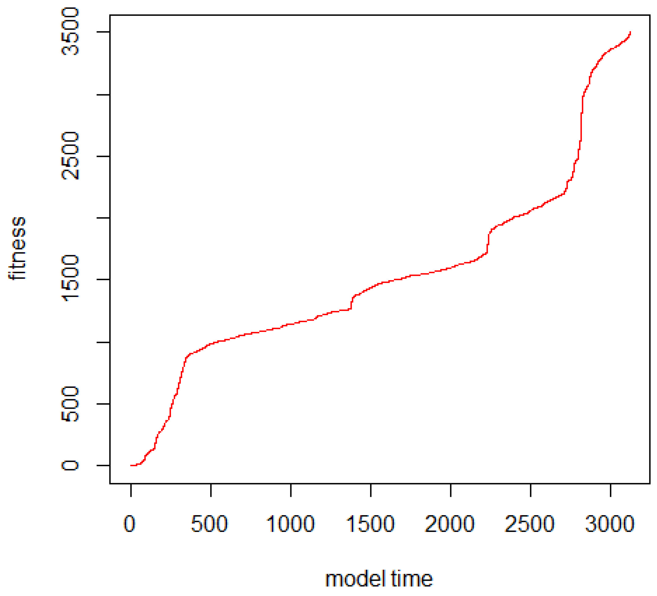
- A genetic algorithm is implemented to evolve the initial population of candidate parameters and to optimize the range of flight parameters.
- Output is produced; this includes coordinates of agents, step-distances, cumulative turn in the respective time step, sinuosity of the flight path, chromosome of the current agent, and the fitness value associated with the current chromosome of the agent.
2.2.4. Design Concepts
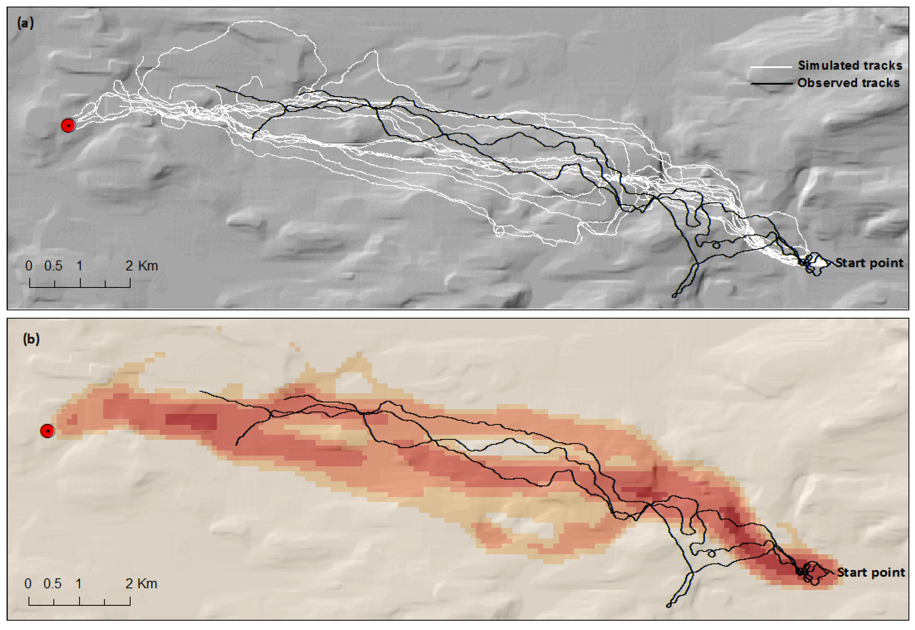
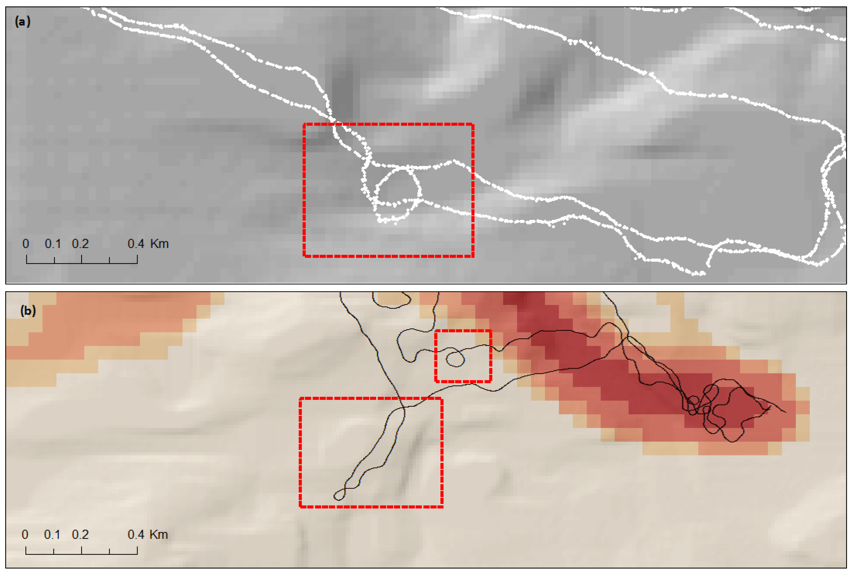
- Emergence: We are interested in a range of parameters that reproduce realistic flight paths and observable navigation behaviours of homing pigeon agents. Specifically, we are looking for observable corridors and possible loops in the flight paths that emerge from navigation, flocking, and random decisions of the pigeons.
- Adaptation: Agents make adaptive decisions during flocking as well as in identifying optimal flight directions by considering the limits of navigation and flocking parameters.
- Objectives: The goal of “simulated” agents is to successfully navigate to the homing loft by following efficient tracks. This is achieved by avoiding areas with abrupt changes in elevation and preferably by navigating in flocks.
- Sensing: Pigeon agents can sense other agents (flock mates) in their neighbourhoods. An agent neighbourhood is specified by visible distance (vision-distance) and a view angle (vision-angle). Additionally, agents can perceive the differences in elevation between their current locations and the surrounding patches in their environments.
- Collectives: Pigeon agents prefer to navigate in flocks, which is a social group of pigeon agents.
- Observation: Apart from the flight paths of agents that are plotted during simulation, additional charts are plotted to show the variation in mean-turn angles, average step-distance, fitness of candidate chromosomes, and sinuosity of flight paths. In addition, a monitor is used to report the cumulative travel time of agents. The flight time (in minutes) is as shown in Equation (1).
2.2.5. Input Data
2.2.6. Sub-Models
2.2.7. Model Parameters
2.2.8. Initialization
2.3. Parameter Estimation and Optimization
3. Results
4. Discussion
5. Conclusions
Acknowledgments
Author Contributions
Conflicts of Interest
References
- An, G.; Mi, Q.; Dutta-Moscato, J.; Vodovotz, Y. Agent-based models in translational systems biology. Wiley Interdiscip. Rev. Syst. Biol. Med. 2009, 1, 159–171. [Google Scholar] [CrossRef] [PubMed]
- Xiang, X.; Kennedy, R.; Madey, G.; Cabaniss, S. Verification and validation of agent-based scientific simulation models. In Proceedings of the Agent-Directed Simulation Conference, New Orleans, LA, USA, 23–28 July 2005.
- Heppenstall, A.; Malleson, N.; Crooks, A. “Space, the final frontier”: How good are agent-based models at simulating individuals and space in cities? Systems 2016, 4, 9. [Google Scholar] [CrossRef]
- Gong, J.; Geng, J.; Chen, Z. Real-time GIS data model and sensor web service platform for environmental data management. Int. J. Health Geogr. 2015, 14, 2. [Google Scholar] [CrossRef] [PubMed]
- Granell, C.; Díaz, L.; Gould, M. Service-oriented applications for environmental models: Reusable geospatial services. Environ. Model. Softw. 2010, 25, 182–198. [Google Scholar] [CrossRef]
- Mineter, M.J.; Jarvis, C.; Dowers, S. From stand-alone programs towards grid-aware services and components: A case study in agricultural modelling with interpolated climate data. Environ. Model. Softw. 2003, 18, 379–391. [Google Scholar] [CrossRef]
- Bröring, A.; Echterhoff, J.; Jirka, S.; Simonis, I.; Everding, T.; Stasch, C.; Liang, S.; Lemmens, R. New generation sensor web enablement. Sensors 2011, 11, 2652–2699. [Google Scholar] [CrossRef] [PubMed]
- Broering, A.; Foerster, T.; Jirka, S.; Priess, C. Sensor bus: an intermediary layer for linking geosensors and the sensor web. In Proceedings of the 1st International Conference and Exhibition on Computing for Geospatial Research & Application, Washington, DC, USA, 21–23 June 2010.
- Song, X.; Wang, C.; Kagawa, M.; Raghavan, V. Real-time monitoring portal for urban environment using sensor web technology. In Proceedings of the 2010 18th International Conference on the Geoinformatics, Beijing, China, 18–20 June 2010.
- Resch, B.; Mittlboeck, M.; Girardin, F.; Britter, R.; Ratti, C. Real-time Geo-awareness–Sensor Data Integration for Environmental Monitoring in the City. In Proceedings of the International Conference on Advanced Geographic Information Systems & Web Services, Cancun, Mexico, 1–7 February 2009.
- Resch, B.; Mittleboeck, M.; Lipson, S.; Welsh, M.; Bers, J.; Britter, R.; Ratti, C.; Blaschke, T. Integrated Urban Sensing: A Geo-Sensor Network for Public Health Monitoring and Beyond; MIT Press: Cambridge, MA, USA, 2011. [Google Scholar]
- Sagl, G.; Blaschke, T.; Beinat, E.; Resch, B. Ubiquitous geo-sensing for context-aware analysis: Exploring relationships between environmental and human dynamics. Sensors 2012, 12, 9800–9822. [Google Scholar] [CrossRef] [PubMed]
- Klug, H.; Kmoch, A. Operationalizing environmental indicators for real time multi-purpose decision making and action support. Ecol. Model. 2015, 295, 66–74. [Google Scholar] [CrossRef]
- Laube, P.; Duckham, M.; Wolle, T. Decentralized movement pattern detection amongst mobile geosensor nodes. In Proceedings of the International Conference on Geographic Information Science, Park City, UT, USA, 23–26 September 2008; Springer: Berlin/Heidelberg, Germany, 2008. [Google Scholar]
- Wikelski, M.; Kays, R. Movebank: Archive, Analysis and Sharing of Animal Movement Data. Available online: http://www.movebank.org (accessed on 17 January 2017).
- Kranstauber, B.; Cameron, A.; Weinzerl, R.; Fountain, T.; Tilak, S.; Wikelski, M.; Kays, R. The Movebank data model for animal tracking. Environ. Model. Softw. 2011, 26, 834–835. [Google Scholar] [CrossRef]
- Dettki, H.; Brode, M.; Clegg, I.; Giles, T.; Hallgren, J. Wireless remote animal monitoring (WRAM)—A new international database e-infrastructure for management and sharing of telemetry sensor data from fish and wildlife. In Proceedings of the 7th International Congress on Environmental Modelling and Software, San Diego, CA, USA, 15–19 June 2014.
- Cagnacci, F.; Urbano, F. Managing wildlife: A spatial information system for GPS collars data. Environ. Model. Softw. 2008, 23, 957–959. [Google Scholar] [CrossRef]
- Urbano, F.; Cagnacci, F.; Calenge, C.; Dettki, H.; Cameron, A.; Neteler, M. Wildlife tracking data management: A new vision. Philos. Trans. R. Soc. B Biol. Sci. 2010, 365, 2177–2185. [Google Scholar] [CrossRef] [PubMed]
- Duckham, M.; Reitsma, F. Decentralized environmental simulation and feedback in robust geosensor networks. Comput. Environ. Urban Syst. 2009, 33, 256–268. [Google Scholar] [CrossRef]
- Duckham, M.; Yeoman, J. Decentralized Algorithms and Simulations for Detecting and Monitoring Convoys. Available online: http://citeseerx.ist.psu.edu/viewdoc/download?doi=10.1.1.716.7594&rep=rep1&type=pdf (accessed on 17 January 2017).
- Darema, F. Dynamic data driven applications systems: A new paradigm for application simulations and measurements. In Proceedings of the Computational Science—ICCS 2004, Kraków, Poland, 6–9 June 2004; Springer: Berlin/Heidelberg, Germany, 2004; pp. 662–669. [Google Scholar]
- Hu, X. Dynamic data driven simulation. SCS M&S Mag. 2011, 1, 16–22. [Google Scholar]
- Akçelik, V.; Biros, G.; Draganescu, A.; Hill, J.; Ghattas, O.; Waanders, B.V.B. Dynamic data-driven inversion for terascale simulations: Real-time identification of airborne contaminants. In Proceedings of the 2005 ACM/IEEE Conference on Supercomputing, Seattle, WA, USA, 12–18 November 2005.
- Gaynor, M.; Seltzer, M.; Moulton, S.; Freedman, J. A dynamic, data-driven, decision support system for emergency medical services. In Proceedings of the Computational Science–ICCS 2005, Atlanta, GA, USA, 22–25 May 2005.
- Celik, N.; Lee, S.; Vasudevan, K.; Son, Y.-J. DDDAS-based multi-fidelity simulation framework for supply chain systems. IIE Trans. 2010, 42, 325–341. [Google Scholar] [CrossRef]
- Pereira, G.M. Dynamic data driven multi-agent simulation. In Proceedings of the IEEE/WIC/ACM International Conference on Intelligent Agent Technology, Fremont, CA, USA, 2–5 November 2007.
- Li, Z.; Guan, X.; Li, R.; Wu, H. 4D-SAS: A Distributed Dynamic-Data Driven Simulation and Analysis System for Massive Spatial Agent-Based Modeling. ISPRS Int. J. Geo-Inf. 2016, 5, 42. [Google Scholar] [CrossRef]
- Rai, S.; Hu, X. Behavior pattern detection for data assimilation in agent-based simulation of smart environments. In Proceedings of the 2013 IEEE/WIC/ACM International Joint Conferences on Web Intelligence (WI) and Intelligent Agent Technologies (IAT), Atlanta, GA, USA, 17–20 November 2013.
- Taormina, R.; Chau, K.-W. Data-driven input variable selection for rainfall–runoff modeling using binary-coded particle swarm optimization and Extreme Learning Machines. J. Hydrol. 2015, 529, 1617–1632. [Google Scholar] [CrossRef]
- Wu, C.L.; Chau, K.W.; Li, Y.S. Methods to improve neural network performance in daily flows prediction. J. Hydrol. 2009, 372, 80–93. [Google Scholar] [CrossRef]
- Zhang, H.; Vorobeychik, Y.; Letchford, J.; Lakkaraju, K. Data-driven agent-based modeling, with application to rooftop solar adoption. Auton. Agents Multi-Agent Syst. 2016, 30, 1023–1049. [Google Scholar] [CrossRef]
- Wallentin, G.; Oloo, F. A Model-sensor Framework to Predict Homing Pigeon Flights in Real Time. GI_Forum 2016, 1, 41–52. [Google Scholar] [CrossRef]
- McLane, A.J.; Semeniuk, C.; McDermid, G.J.; Marceau, D.J. The role of agent-based models in wildlife ecology and management. Ecol. Model. 2011, 222, 1544–1556. [Google Scholar] [CrossRef]
- Bennett, D.A.; Tang, W. Modelling adaptive, spatially aware, and mobile agents: Elk migration in Yellowstone. Int. J. Geogr. Inf. Sci. 2006, 20, 1039–1066. [Google Scholar] [CrossRef]
- Hamblin, S.; Giraldeau, L.-A. Finding the evolutionarily stable learning rule for frequency-dependent foraging. Anim. Behav. 2009, 78, 1343–1350. [Google Scholar] [CrossRef]
- Hamblin, S. On the practical usage of genetic algorithms in ecology and evolution. Methods Ecol. Evol. 2013, 4, 184–194. [Google Scholar] [CrossRef]
- Okunishi, T.; Yamanaka, Y.; Ito, S.-I. A simulation model for Japanese sardine (Sardinops melanostictus) migrations in the western North Pacific. Ecol. Model. 2009, 220, 462–479. [Google Scholar] [CrossRef]
- Kawecki, T.J.; Ebert, D. Conceptual issues in local adaptation. Ecol. Lett. 2004, 7, 1225–1241. [Google Scholar] [CrossRef]
- Wechsler, B.; Lea, S.E. Adaptation by learning: Its significance for farm animal husbandry. Appl. Anim. Behav. Sci. 2007, 108, 197–214. [Google Scholar] [CrossRef]
- Lauer, M.; Riedmiller, M. An algorithm for distributed reinforcement learning in cooperative multi-agent systems. In Proceedings of the Seventeenth International Conference on Machine Learning, Stanford, CA, USA, 29 June–2 July 2000.
- Macal, C.M.; North, M.J. Tutorial on agent-based modelling and simulation. J. Simul. 2010, 4, 151–162. [Google Scholar] [CrossRef]
- Stonedahl, F.; Wilensky, U. Finding forms of flocking: Evolutionary search in abm parameter-spaces. In Proceedings of the International Workshop on Multi-Agent Systems and Agent-Based Simulation, Toronto, ON, Canada, 11 May 2010; Springer: Berlin/Heidelberg, Germany, 2010. [Google Scholar]
- Stonedahl, F.; Rand, W.M. When Does Simulated Data Match Real Data? Comparing Model Calibration Functions Using Genetic Algorithms; Robert H. Smith School Research Paper No. RHS-06-151; University of Maryland: College Park, MD, USA, 2012. [Google Scholar]
- Stonedahl, F.; Wilensky, U. Evolutionary robustness checking in the artificial anasazi model. In Proceedings of the AAAI Fall Symposium: Complex Adaptive Systems, Arlington, VA, USA, 11–13 November 2010.
- Holland, J.H. Complex Adaptive Systems; Daedalus; The MIT Press: Cambridge, MA, USA, 1992. [Google Scholar]
- Holland, J.H. Adaptation in Natural and Artificial Systems: An Introductory Analysis with Applications to Biology, Control, and Artificial Intelligence; University of Michigan Press: Ann Arbor, MI, USA, 1975. [Google Scholar]
- Mitchell, M. Genetic algorithms: An overview. Complexity 1995, 1, 31–39. [Google Scholar] [CrossRef]
- Mitchell, M. An Introduction to Genetic Algorithms; MIT Press: Cambridge, MA, USA, 1998. [Google Scholar]
- Calvez, B.; Hutzler, G. Automatic tuning of agent-based models using genetic algorithms. In Proceedings of the International Workshop on Multi-Agent Systems and Agent-Based Simulation, Paris, France, 4–6 July 2005; Springer: Berlin/Heidelberg, Germany, 2005. [Google Scholar]
- Barta, Z.; Flynn, R.; Giraldeau, L.-A. Geometry for a selfish foraging group: A genetic algorithm approach. Proc. R. Soc. Lond. B Biol. Sci. 1997, 264, 1233–1238. [Google Scholar] [CrossRef]
- Beauchamp, G. A spatial model of producing and scrounging. Anim. Behav. 2008, 76, 1935–1942. [Google Scholar] [CrossRef]
- Oremland, M.; Laubenbacher, R. Optimization of agent-based models: Scaling methods and heuristic algorithms. J. Artif. Soc. Soc. Simul. 2014, 17, 6. [Google Scholar] [CrossRef]
- Mandel, J.; Beezley, J.D.; Bennethum, L.S.; Chakraborty, S.; Coen, J.L.; Douglas, C.C.; Hatcher, J.; Kim, M.; Vodacek, A. A dynamic data driven wildland fire model. In Proceedings of the International Conference on Computational Science, Beijing, China, 27–30 March 2007; Springer: Berlin/Heidelberg, Germany, 2007. [Google Scholar]
- Rodríguez, R.; Cortés, A.; Margalef, T. Injecting dynamic real-time data into a DDDAS for forest fire behavior prediction. In Proceedings of the International Conference on Computational Science, Vancouver, BC, Canada, 29–31 August 2009; Springer: Berlin/Heidelberg, Germany, 2009. [Google Scholar]
- Denham, M.; Cortés, A.; Margalef, T.; Luque, E. Applying a Dynamic Data Driven Genetic Algorithm to Improve Forest Fire Spread Prediction. In Proceedings of the 8th International Conference on Computational Science, Kraków, Poland, 23–25 June 2008; Bubak, M., van Albada, G.D., Dongarra, J., Sloot, P.M.A., Eds.; Springer: Berlin/Heidelberg, Germany, 2008; pp. 36–45. [Google Scholar]
- Lee, K.H.; Choi, M.G.; Hong, Q.; Lee, J. Group behavior from video: A data-driven approach to crowd simulation. In Proceedings of the 2007 ACM SIGGRAPH/Eurographics Symposium on Computer Animation, San Diego, CA, USA, 3–4 August 2007.
- Nagy, M.; Akos, Z.; Biro, D.; Vicsek, T. Hierarchical group dynamics in pigeon flocks. Nature 2010, 464, 890–893. [Google Scholar] [CrossRef] [PubMed]
- Blaser, N.; Dell′Omo, G.; Dell′Ariccia, G.; Wolfer, D.P.; Lipp, H.P. Testing cognitive navigation in unknown territories: Homing pigeons choose different targets. J. Exp. Biol. 2013, 216, 3123–3131. [Google Scholar] [CrossRef] [PubMed] [Green Version]
- Santos, C.D.; Neupert, S.; Lipp, H.-P.; Wikelski, M.; Dechmann, D.K. Temporal and contextual consistency of leadership in homing pigeon flocks. PLoS ONE 2014, 9, e102771. [Google Scholar] [CrossRef] [PubMed]
- Santos, C.D.; Neupert, S.; Lipp, H.-P.; Wikelski, M.; Dechmann, D. Data from: Temporal and Contextual Consistency of Leadership in Homing Pigeon Flocks. Available online: https://www.datarepository.movebank.org/handle/10255/move.365 (accessed on 10 October 2016).
- Grimm, V.; Berger, U.; DeAngelis, D.L.; Polhill, J.G.; Giske, J.; Railsback, S.F. The ODD protocol: A review and first update. Ecol. Model. 2010, 221, 2760–2768. [Google Scholar] [CrossRef]
- Wilensky, U. NetLogo (and NetLogo User Manual); Center for Connected Learning and Computer-Based Modeling, Northwestern University: Evanston, IL, USA, 1999. [Google Scholar]
- Arundel, J.; Oldroyd, B.P.; Winter, S. Modelling honey bee queen mating as a measure of feral colony density. Ecol. Model. 2012, 247, 48–57. [Google Scholar] [CrossRef]
- Polhill, J.G.; Parker, D.; Brown, D.; Grimm, V. Using the ODD protocol for describing three agent-based social simulation models of land-use change. J. Artif. Soc. Soc. Simul. 2008, 11, 3. [Google Scholar]
- Tang, W.; Bennett, D.A. Agent-based modeling of animal movement: A review. Geogr. Compass 2010, 4, 682–700. [Google Scholar] [CrossRef]
- Reynolds, C.W. Flocks, herds and schools: A distributed behavioral model. In ACM SIGGRAPH Computer Graphics; ACM: New York, NY, USA, 1987. [Google Scholar]
- Wilensky, U. NetLogo Flocking Model; Center for Connected Learning and Computer-Based Modeling, Northwestern University: Evanston, IL, USA, 1998. [Google Scholar]
- Mitchell, M.T.; Wilensky, U. NetLogo Robby the Robot Model; Center for Connected Learning and Computer-Based Modeling, Northwestern University: Evanston, IL, USA, 2012. [Google Scholar]
- Noraini, M.R.; Geraghty, J. Genetic algorithm performance with different selection strategies in solving TSP. In Proceedings of the World Congress on Engineering, London, UK, 6–8 July 2011.
- Goldberg, D.E.; Deb, K. A comparative analysis of selection schemes used in genetic algorithms. Found. Genet. Algorithms 1991, 1, 69–93. [Google Scholar]
- Walter, W.D.; Fischer, J.W.; Baruch-Mordo, S.; VerCauteren, K.C. What Is the Proper Method to Delineate Home Range of An Animal Using Today’s Advanced GPS Telemetry Systems: The Initial Step; InTech: Rijeka, Croatia, 2011. [Google Scholar]
- Downs, J.; Horner, M. Network-based kernel density estimation for home range analysis. In Proceedings of the Ninth International Conference on Geocomputation, Maynooth, Ireland, 3–5 September 2007.
- Dell’Ariccia, G.; Dell’Omo, G.; Wolfer, D.P.; Lipp, H.-P. Flock flying improves pigeons’ homing: GPS track analysis of individual flyers versus small groups. Anim. Behav. 2008, 76, 1165–1172. [Google Scholar] [CrossRef] [Green Version]
- Grimm, V.; Revilla, E.; Berger, U.; Jeltsch, F.; Mooij, W.M.; Railsback, S.F.; Thulke, H.-H.; Weiner, J.; Wiegand, T.; DeAngelis, D.L. Pattern-oriented modeling of agent-based complex systems: Lessons from ecology. Science 2005, 310, 987–991. [Google Scholar] [CrossRef] [PubMed]
- Beasley, D.; Martin, R.; Bull, D. An overview of genetic algorithms: Part 1. Fundamentals. Univ. Comput. 1993, 15, 58. [Google Scholar]
- El-Mihoub, T.A.; Hopgood, A.A.; Nolle, L.; Battersby, A. Hybrid Genetic Algorithms: A Review. Eng. Lett. 2006, 13, 124–137. [Google Scholar]
- Wendt, K.; Cortés, A.; Margalef, T. Knowledge-guided genetic algorithm for input parameter optimisation in environmental modelling. Procedia Comput. Sci. 2010, 1, 1367–1375. [Google Scholar] [CrossRef]
- Whitsed, R.; Smallbone, L.T. A hybrid genetic algorithm with local optimiser improves calibration of a vegetation change cellular automata model. Int. J. Geogr. Inf. Sci. 2016, 1–21. [Google Scholar] [CrossRef]
- Sajjad, M.; Singh, K.; Paik, E.; Ahn, C.-W. A Data-Driven Approach for Agent-Based Modeling: Simulating the Dynamics of Family Formation. J. Artif. Soc. Soc. Simul. 2016, 19, 1–14. [Google Scholar] [CrossRef]
- Ward, J.A.; Evans, A.J.; Malleson, N.S. Dynamic calibration of agent-based models using data assimilation. R. Soc. Open Sci. 2016, 3, 150703. [Google Scholar] [CrossRef] [PubMed]
- Lee, J.-S.; Filatova, T.; Ligmann-Zielinska, A.; Hassani-Mahmooei, B.; Stonedahl, F.; Lorscheid, I.; Voinov, A.; Polhill, J.G.; Sun, Z.; Parker, D.C. The Complexities of Agent-Based Modeling Output Analysis. J. Artif. Soc. Soc. Simul. 2015, 18. [Google Scholar] [CrossRef]
- Nittel, S. A Survey of Geosensor Networks: Advances in Dynamic Environmental Monitoring. Sensors 2009, 9, 5664–5678. [Google Scholar] [CrossRef] [PubMed]
- Gross, M. Animal moves reveal bigger picture. Curr. Biol. 2015, 25, R585–R588. [Google Scholar] [CrossRef] [PubMed]


| Homing Flight | Number of Data Points | Number of Birds |
|---|---|---|
| 1 | 4667 | 8 |
| 2 | 2788 | 8 |
| 3 | 3500 | 7 |
| 4 | 3496 | 8 |
| 5 | 3844 | 9 |
| Sub-Model | Purpose |
|---|---|
| read-GPS-sensor? | Uses emulated GPS points to create and to guide navigation of “real” agents. |
| create-birds-agents | Uses the first set of coordinates in the emulated GPS tracks to create “simulated” pigeon agents. Additionally, sets the initial state variables of simulated agents. |
| display-elevation | Imports the DEM, transforms its coordinates to the model coordinate system, and specifies how the environment is displayed. |
| map-turn | Uses a defined elevation turn (max-elevation-turn) and the variation of elevation in the locality of an agent to re-orient the heading of the agent. |
| compass-turn | An agent uses trigonometric functions to determine the bearing to the home loft. The result is compared to the allowable compass turn (max-loft-turn), if the bearing is less than max-loft-turn then the agent reorients its heading to face the direction of the home loft otherwise the agent turns by an angle that is equivalent to the max-loft-turn in the direction of the home loft. |
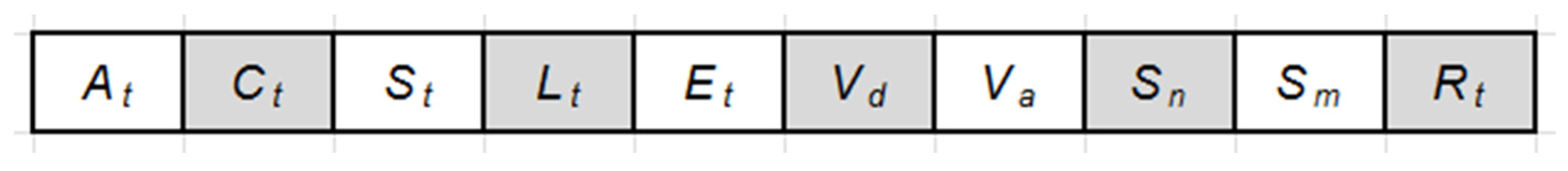
| encode-chromosome | Uses a predefined set of model parameters to encode a vector of candidate chromosomes; stochasticity is introduced in the chromosomes by using a normal distribution with a mean of 0.0 and standard deviation of 0.01 to randomly vary the individual chromosome parameters. |
| create-new-generation | Implements genetic algorithm operators of selection, crossover, mutation, and replacement. |
| mutate | Randomly selects a gene within the candidate (intermediate) chromosome and uses a normal distribution with a mean of 0.0 and standard deviation of 0.1 to vary the selected gene. |
| export-results | Generates a tabular output of the agent properties at each time step. |
| Parameter | Description | Base Values |
|---|---|---|
| max-align-turn | Maximum turning angle that an agent can execute to align to flight direction of flock mates. | 8.0 |
| max-cohere-turn | Maximum turning angle that an agent can implement to be in coherence with its flock mates. | 11.0 |
| max-elevation-turn | Maximum turning angle that an agent can perform in order to fly along a controlled topographic contour. | 3.7 |
| max-loft-turn | Maximum turn angle that an agent can make in order to fly in a general bearing towards the home loft. | 1.9 |
| max-separation-turn | Maximum turning that an agent performs in order to be in separate from nearby flock mates. | 3.5 |
| max-step-distance | Maximum distance that an agent can traverse in a single time step. | |
| minimum-separation-m | Least distance that is necessary to avoid collision between pigeons in a flock. | 1.25 |
| min-step-distance | Least distance that an agent can traverse in a single time step in order to continue with navigation. | |
| mutation-rate | Rate at which mutation in candidate chromosomes occur. | 0.01 |
| random-turn-prob | Probability of an agent making a random turn. | 0.3 |
| replace-proportion | Proportion of candidate agents that are replaced in each time step. | 0.6 |
| view-angle | Maximum angular radius that is viewable to an agent at any instance. | 340 |
| vision-m | Maximum distance that is visible to an agent at any instance. | 100 |
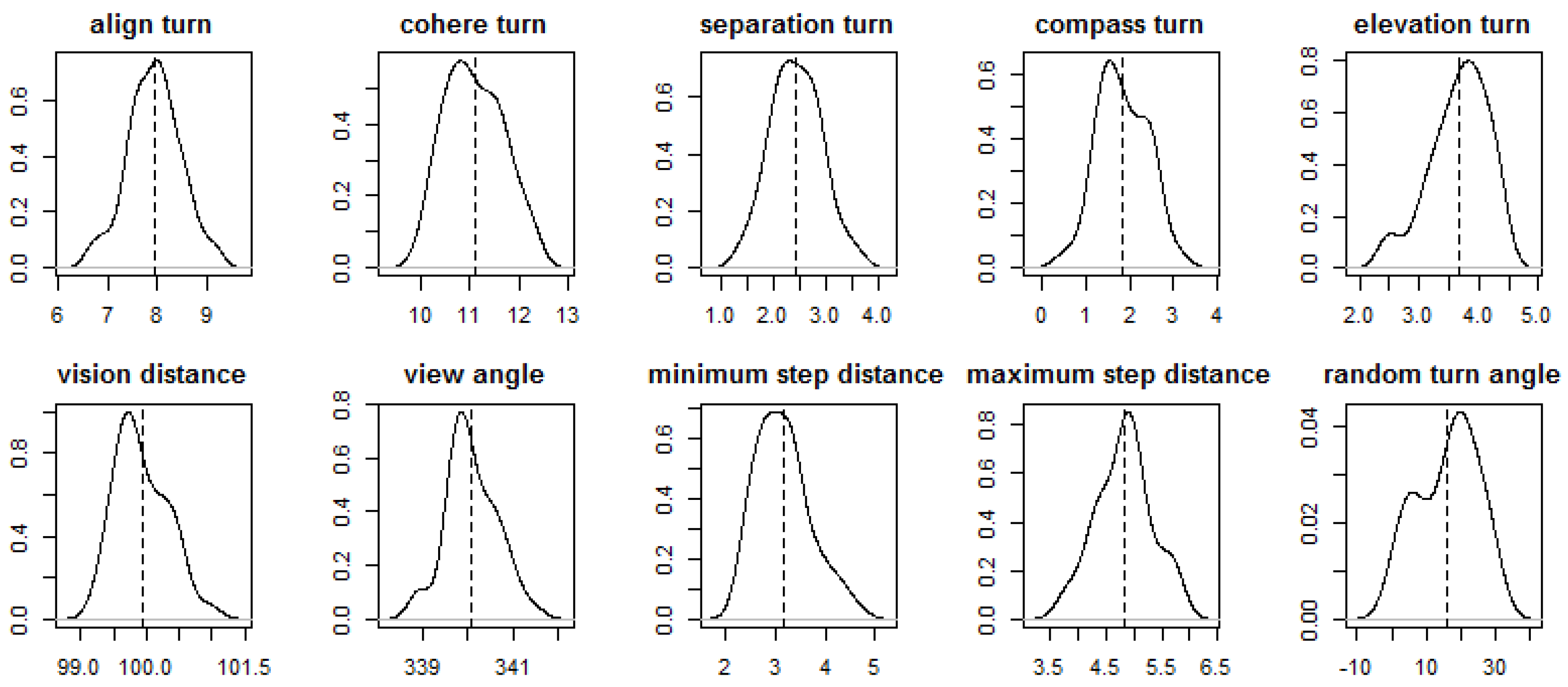
| Parameters | Mean (95% CI) |
|---|---|
| maximum alignment turn angle | 8.01 (7.87–8.16) |
| maximum cohere turn angle | 10.93 (10.81–11.04) |
| maximum separation turn angle | 2.36 (2.22–2.51) |
| maximum compass turn angle | 1.94 (1.82–2.06) |
| maximum elevation turn angle | 3.63 (3.47–3.78) |
| vision distance | 100.05 (99.9–100.2) |
| view angle | 340 (339.8–340.1) |
| minimum step distance | 2.45 (2.34–2.56) |
| maximum step distance | 7.07 (6.8–7.35) |
| random turn angle | 14.72 (12.29–17.16) |
© 2017 by the authors; licensee MDPI, Basel, Switzerland. This article is an open access article distributed under the terms and conditions of the Creative Commons Attribution (CC BY) license (http://creativecommons.org/licenses/by/4.0/).
Share and Cite
Oloo, F.; Wallentin, G. An Adaptive Agent-Based Model of Homing Pigeons: A Genetic Algorithm Approach. ISPRS Int. J. Geo-Inf. 2017, 6, 27. https://doi.org/10.3390/ijgi6010027
Oloo F, Wallentin G. An Adaptive Agent-Based Model of Homing Pigeons: A Genetic Algorithm Approach. ISPRS International Journal of Geo-Information. 2017; 6(1):27. https://doi.org/10.3390/ijgi6010027
Chicago/Turabian StyleOloo, Francis, and Gudrun Wallentin. 2017. "An Adaptive Agent-Based Model of Homing Pigeons: A Genetic Algorithm Approach" ISPRS International Journal of Geo-Information 6, no. 1: 27. https://doi.org/10.3390/ijgi6010027