Evaluating Temporal Analysis Methods Using Residential Burglary Data

Abstract

Law enforcement agencies, as well as researchers rely on temporal analysis methods in many crime analyses, e.g., spatio-temporal analyses. A number of temporal analysis methods are being used, but a structured comparison in different configurations is yet to be done. This study aims to fill this research gap by comparing the accuracy of five existing, and one novel, temporal analysis methods in approximating offense times for residential burglaries that often lack precise time information. The temporal analysis methods are evaluated in eight different configurations with varying temporal resolution, as well as the amount of data (number of crimes) available during analysis. A dataset of all Swedish residential burglaries reported between 2010 and 2014 is used (N = 103,029). From that dataset, a subset of burglaries with known precise offense times is used for evaluation. The accuracy of the temporal analysis methods in approximating the distribution of burglaries with known precise offense times is investigated. The aoristic and the novel aoristic${}_{ext}$ method perform significantly better than three of the traditional methods. Experiments show that the novel aoristic${}_{ext}$ method was most suitable for estimating crime frequencies in the day-of-the-year temporal resolution when reduced numbers of crimes were available during analysis. In the other configurations investigated, the aoristic method showed the best results. The results also show the potential from temporal analysis methods in approximating the temporal distributions of residential burglaries in situations when limited data are available.

1. Introduction

When investigating and analyzing crimes, it is important to have precise temporal information. Whilst aggregating burglaries might show an increase of crimes on certain weekdays, the temporal analysis might indicate more complex patterns, as the temporal resolution is changed, e.g., from days to hours. Further, the temporal information of different crime categories conveys different information about the crime category or about the perpetrator, e.g., when a crime was committed might help rule out a large group of possible perpetrators. As such, having precise temporal information available is important to law enforcement agencies during, e.g., spatio-temporal analyses or hotspot analyses.

However, crime data often contain uncertainties, e.g., if the crime was committed without any witnesses, it might be difficult to collect complete, precise information. Some crime categories, e.g., unattended property theft, such as burglaries, often lack precise temporal information. They are often reported to have taken place sometime within a time interval of various length [1,2]. The lack of accurate temporal data regarding certain crime types is unfortunate, since it renders the analysis of crime more difficult [3]. Consequently, there is a need for methods with the ability to, based on imprecise temporal data, estimate a more accurate time of occurrence for offenses.

Estimating the actual time of occurrence can be resource demanding, as the number of crimes available and the temporal resolution vary, e.g., hour of the day or month in the year. There exist multiple methods for estimating the occurrence time of a crime [1]. The estimated occurrence times are affected by the estimation method used. However, no thorough comparison of existing methods in different temporal configurations has been conducted within the research community.

The present study therefore sets out to fill this research gap by evaluating five existing methods, and one novel method, in order to determine which methods most accurately estimate temporal patterns given different temporal resolutions and crime sample sizes. Choosing a suitable method is important, as the choice of method affects the end analysis result and, thereby, also law enforcement agencies’ ability to perform crime analysis, as well as their knowledge concerning temporal crime patterns.

1.1. Aim and Scope

The aim of this study is to investigate which of six temporal analysis methods most accurately approximates the temporal distribution of residential burglaries with known precise offense times in various temporal configurations. The evaluations are made with respect to the following four temporal resolutions: (1) hour of the day; (2) day of the week; (3) month of the year and (4) day of the year. For each of these temporal resolutions, the temporal analysis methods are investigated using both a dataset that contains all available burglary data, as well as a dataset with samples of the offenses, i.e., only a limited number of cases included in the analysis. Thus, each temporal analysis method is evaluated in eight configurations with both varying temporal resolution and amount of available burglary data during analysis. It should be emphasized that the main result from this study is not the temporal patterns created from the data, but rather the performance of the investigated temporal analysis methods in predicting the temporal distribution in various temporal configurations, i.e., in different temporal resolutions and crime sample sizes.

The scope of this study is limited to the evaluation of the performance of six temporal analysis methods on a dataset that consists of all reported Swedish residential burglaries between 2010 and 2014. All methods will be evaluated on the eight configurations described above.

1.2. Outline

In the next section, the related work is presented, followed by the introduction of the six temporal analysis methods in Section 3. Then, the dataset used is described in Section 4, and the experiments in which the performance of the analysis methods are evaluated are introduced in Section 5. The results from the experiments are presented in Section 6 and analyzed in Section 7. Finally, Section 8 concludes the work and presents future work.

2. Related Work

Analytical methods for predicting crimes include approaches for making use of historical crime data, e.g., crime mapping, hot spot identification and risk terrain analysis [2,3,4,5]. The impact of hurricanes on burglaries has also been investigated [6]. Within environmental criminology, [7] study environmental factors influencing criminal activities. Other important approaches involve repeat, or near-repeat, victimization, as well as spatio-temporal analysis methods [3]. The work in [8] investigates 10 cities in five countries and finds that the risk of residential burglary is temporarily increased for at least two weeks within a 200-m radius around burgled residences. Research into criminal behavior involves using journey-to-crime theory to suggest how burglars are likely to identify target houses prior to offending [9,10]. As such, targets are more likely to be located close to an area familiar to the offender.

A majority of the previous research has been focused on methods involving the analysis of spatial data, leaving temporal analysis methods less explored [11,12]. However, this does not imply that temporal data are of less importance from a crime prediction perspective [13,14].

The work in [15] investigates how temporal information can be represented according to five categories: moments, duration, structured time, time as distance and space as clock. The latter can be used to depict how an area changes over time (e.g., a seasonal map). However, the previous four categories are considered more interesting for crime analysis and prediction [3]. A moment is a singular point in time, often when something happened. This could be an estimated point or a known exact time. A duration of time is the time between two points, e.g., the event is estimated to have happened between time x and y. Time as distance is the measurement of how far it would be possible to travel within a time duration, e.g., a light year [3]. Finally, structured time is the representation of time as, e.g., minutes and hours. More specifically, it is the structuring of time into pieces that are more easily managed.

In addition to the five temporal categories listed above, time span has been identified as another time representation. Time span is a duration in which a moment or a duration could have taken place, but one is unsure about the specifics [3]. Although offenses have durations themselves, e.g., the offense took 10 minutes to perform, they are often regarded as moments since these durations for burglaries are considerably shorter compared to the time spans in which the offenses have occurred.

Studies on the temporal characteristics of different types of crimes have been conducted to increase the understanding of criminal behavior, e.g., when offenders commit crimes [14,16]. For instance, offenses have been found to be more likely to be committed in the afternoon or early evening [11,13], while nighttime burglaries were found to be more likely during weekends [17]. This would suggest that knowledge of victim behavior is essential to the criminal behavior, e.g., late mornings and early afternoon are more likely to result in empty houses due to work hours. This is also supported by the routine activity theory, i.e., that offenders identify opportunities during routine activities, such as driving to work [13].

Reported household disturbances are found to increase during holidays compared to other days [18]. The rationale behind this is in the line of routine activities and that changes in regular activities lead to increased risk of victimization [17]. Furthermore, various types of crimes have been studied in relation to national holidays in a U.S. setting [19]. It is concluded that crime rates vary not only with the type of holiday, but also with the type of crime. During major holidays, increased frequencies of violent crimes are reported, while the opposite is true for property crimes. It is hypothesized that minor holidays have little or no impact on crime rates. The routine activity theory indicates that only holidays that influence peoples’ regular activities should have an effect on crime rates, i.e., major holidays should have a larger influence compared to minor holidays.

Producing accurate temporal maps of when crimes occur is a difficult task [2]. Nevertheless, several methods exist that can represent crimes either as moments or to account for the estimated time spans. Circular statistics has been used when analyzing the number of incidents reported to the police by time of the day and day of the week [20]. Further, the temporal distribution of offenses has been investigated by mapping the crimes into quartile minutes [13]. This allows the comparison of the crime time distribution between cities and geographical areas.

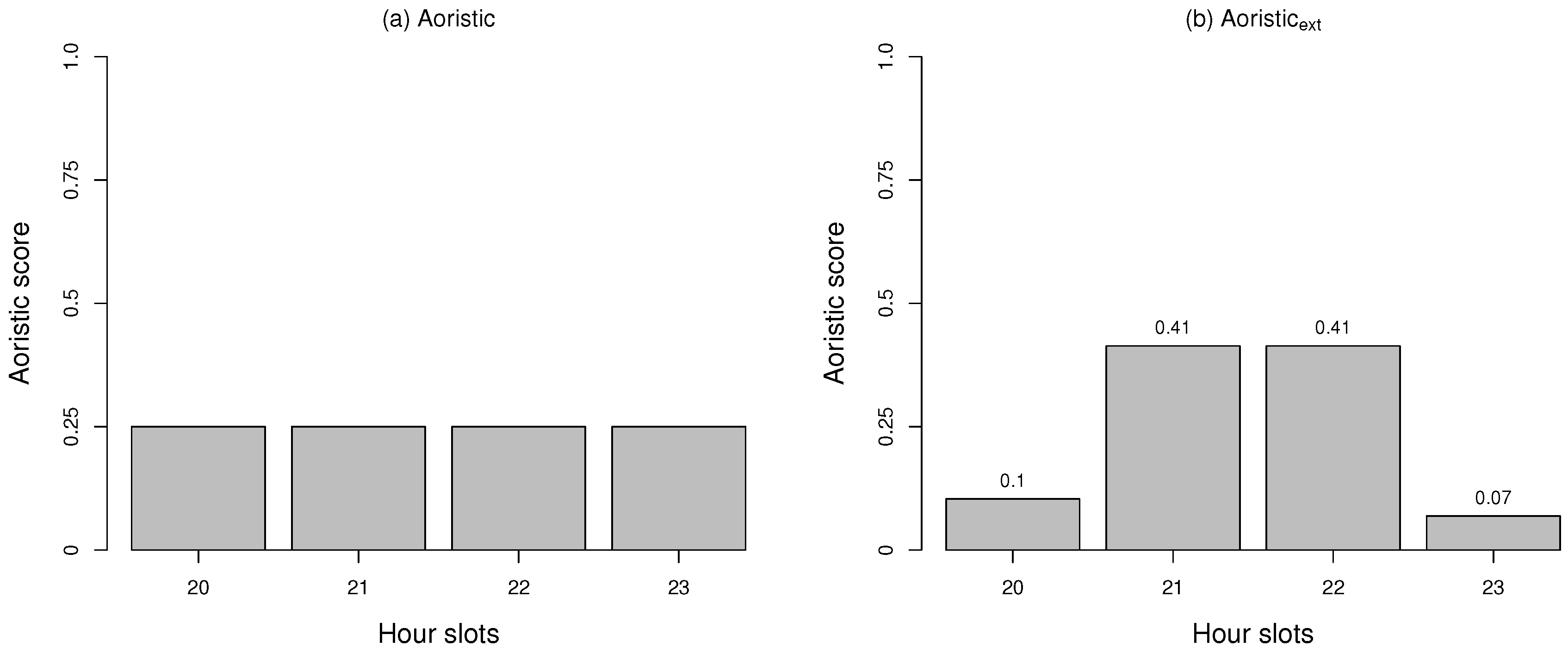
One temporal analysis method often included in crime analytics software is the aoristic method that can handle crimes without a known specific occurrence time, i.e., represented as a time span instead [1,12,16]. It works by choosing a structured time or temporal unit, e.g., hours or days. It works by giving each offense a point of $1.0$, which then is evenly divided among the units within the time span. This is repeated for every crime investigated. The points of every temporal unit are then summarized and used to indicate high profile time periods, which evenly distributes the likelihood of when a crime occurred across the possible temporal units.

The accuracy of temporal analysis methods has been evaluated on their ability to estimate the exact offense time for bicycle thefts [11]. The study evaluates how accurately five methods can estimate the true offense time in terms of hour of the day. It was concluded that the aoristic method best manages to estimate the offense time in that context. However, the study does not evaluate the methods in different configurations and only includes 303 crimes in the analysis.

Research gaps identified within the present study include a lack of the evaluation of temporal analysis methods over multiple temporal resolutions, e.g., months in the year or hour in the day. Single types of structured time have been evaluated on different types of crimes, e.g., bicycle and car thefts, as well as assaults [11,12]. The functionality of the aoristic method does not take into account whether time slots are fully or only partially covered when distributing the point, e.g., if the temporal resolution is days, then the aoristic method does not consider whether a certain day is fully covered or not. That is, a time slot that is only covered marginally is given the same amount of points as a time slot that is fully covered. Finally, previous work has to a large extent been studied within the U.S. and U.K. contexts.

3. Temporal Analysis Methods

In this section, the temporal analysis methods evaluated in this study are defined. Before the analysis methods are introduced, some temporal concepts need to be defined.

3.1. Definitions of Temporal Concepts

The following nine temporal concepts/properties are associated with most property-related offenses, including residential burglaries:

• $dat{e}_{start}$ denotes the first date on which an offense could have occurred.
• $dat{e}_{end}$ denotes the last date on which an offense could have occurred; always the same or a later date than $dat{e}_{start}$.
• $tim{e}_{start}$ denotes the first time an offense could have occurred on a certain date.
• $tim{e}_{end}$ denotes the last time an offense could have occurred on a certain date.
• $offens{e}_{start}$ denotes the first moment in time, measured in seconds, that an offense could have occurred. It is a combination of both a date and a time within that date expressed as: $\{dat{e}_{start},tim{e}_{start}\}$.
• $offens{e}_{end}$ denotes the last moments in time that an offense could have occurred. It is a combination of both a date and a time within that date expressed as: $\{dat{e}_{end},tim{e}_{end}\}$.
• $offens{e}_{duration}$ denotes the time duration during which an offense could have occurred, measured in seconds. It is calculated according to Equation (1).

  $$offense{s}_{duration}=offens{e}_{end}-offens{e}_{start}$$

  (1)

3.2. Introduction of Temporal Analysis Methods

Five existing temporal analysis methods and one new method are introduced below. These methods approximate the real, but unknown occurrence times of burglaries, using $offens{e}_{start}$ and $offens{e}_{end}$.

• The start method is trivial in its functionality as it simply regards the occurrence time to be the same as $offens{e}_{start}$. A major shortcoming attributed to this method is that $offens{e}_{start}$ is not more likely than any other moment included within $offens{e}_{duration}$.
• The end method works similarly as the start method, but it instead regards the offense time to be $offens{e}_{end}$.
• The average method approximates the offense time to be in the middle of $offens{e}_{start}$ and $offens{e}_{end}$ as expressed in Equation (2) below. Similarly to the shortcoming of the start and stop methods, the moment in time approximated by the average method is not more likely than any other within $offens{e}_{duration}$.

  $$offens{e}_{average}=offens{e}_{start}+\frac{offens{e}_{duration}}{2}$$

  (2)
• The random method uniformly selects a moment in time within the time span bounded by $offens{e}_{start}$ and $offens{e}_{end}$ (inclusive) [11]. Just as for the previous methods, there is nothing that makes the moment in time selected more probable than any other moments within $offens{e}_{duration}$. However, since any time within the time span is a candidate, the method can potentially approximate the temporal distribution of burglaries with a known offense time if sufficiently many data points are included in the analysis based on the law of large numbers.
• The aoristic method creates a time span by dividing the time into slots based on the unit of analysis, e.g., hour or day. Next, a score of $1.0$ is assigned to the offense and divided evenly across the slots covered by $offens{e}_{duration}$ [1]. This division is done regardless of whether the slots are fully or partially covered, as shown in Equation (3), in which n represents the number of slots covered.

  $$aoristic=\frac{1.0}{n}$$

  (3)
• Aoristic${}_{ext}$ is a novel method presented in this work. It works by creating a time span using the same approach as the aoristic method, with the exception that it takes into account whether time slots are fully or only partially covered when calculating the aoristic score. It first calculates the total coverage of the slots that the offense spans either partly or completely according to Equation (4), where $coverag{e}_i$ is the coverage of slot i expressed as a value between zero and one, and n is the total number of slots.

  $$coverag{e}_{total}=\sum _{i=1}^{n}coverag{e}_i$$

  (4)

  Next, the score for each slot is calculated by dividing the coverage of that slot with the total coverage, as shown in Equation (5). The sum of the scores for all slots always equals $1.0$.

  $$scor{e}_i=\frac{coverag{e}_i}{coverag{e}_{total}}$$

  (5)

As an example, consider a burglary reported to have occurred somewhere between 20:45 and 23:10. It can be concluded that the offense covers four different hours, although only two of them is fully covered. Both start and stop methods will assign full scores ($1.0$) to the first and last slot, respectively. The average method will assign a full score to the second slot since the average time between start and stop is 21:57:30, i.e., the moment falls within the second hour. The random method will assign a full score to any of the four slots based on a uniform distribution.

The aoristic method calculates its score by dividing the point available for the offense with the number of time slots covered. Since the example burglary spans four slots, $n=4$, each of these slots will receive a score of $1/4=0.25$, as shown in Figure 1a.

The aoristic${}_{ext}$ method starts by determining the total coverage of all slots, which is $15+60+60+10=145$ min, but in practice, seconds rather than minutes are used. Then, the score for each slot in the example is the fraction it covers. The first slot is calculated as $15/145\approx 0.10$, the second and third slot as $60/145\approx 0.41$ and, finally, the fourth slot as $10/145\approx 0.07$, as shown in Figure 1b. Consequently, the aoristic${}_{ext}$ method takes into account more detailed temporal information when establishing the scores compared to the traditional aoristic method.

4. Data

In this section, the data collection, representation and cleaning processes that this study relies on are described. The temporal analysis methods are evaluated on official criminal records of residential burglaries provided by the Swedish police. Both attempted and completed burglaries were included. Attempted burglaries were included because they indicate the offender’s objective to gain unlawful entrance to a residence, although the burglaries were interrupted. In the remainder of this work, the term burglaries refers to both completed and attempted burglaries.

The dataset consists of all burglaries registered in Sweden during five years, from 1 January 2010 to 31 December 2014. A total of 103,029 burglaries are included in the dataset.

4.1. Data Cleaning

As shown in

Table 1. Number of burglaries per year included in this study and the number of removed records per year.

	2010	2011	2012	2013	2014	Total
Number of burglaries	19 798	22 242	21 449	21 078	22 453	107 020
Missing data	482	496	836	859	871	3 544
Erroneous temporal data	143	201	24	38	41	447
Burglaries in dataset	19 173	21 545	20 589	20 181	21 541	103 029

, roughly 3.7% of the data records were removed from the dataset due to inconsistencies or missing attributes. These records were removed due to either:

• missing attribute, e.g., missing temporal attribute, or
• erroneous temporal attribute, e.g., start time greater than end time.

Inconsistencies in the records were most likely due to human error introduced when filing out the criminal reports. No patterns in how the erroneous records were dispersed in the dataset were found, i.e., they were not grouped at any particular time intervals. Therefore, the erroneous records are assumed to be uniformly distributed throughout the dataset. Although, such errors are slightly more common in 2012–2014 compared to the earlier years. After inconsistent data records were removed, a total of 103,029 burglaries remained, and they make up the dataset used in this study; see Table 1. The process of cleaning crime records was carried out in the statistical software suite R.

4.2. Data Representation

Each burglary in the dataset is represented using four attributes. The attributes, listed in

Table 2. Type and format of instances’ attributes.

	Type	Format	Comment
$dat{e}_{start}$	Date	yyyy-mm-dd	Denotes first possible offense date
$dat{e}_{end}$	Date	yyyy-mm-dd	Denotes last possible offense date
$tim{e}_{start}$	Time	hh:mm:ss	Denotes first possible offense time
$tim{e}_{end}$	Time	hh:mm:ss	Denotes last possible offense time

, are similar to the temporal concepts explained in Section 3. $dat{e}_{start}$ denotes the first date on which an offense could have occurred, while $dat{e}_{end}$ denotes the last date. Similarly, the times $tim{e}_{start}$ and $tim{e}_{end}$ denote the first and last time on a certain date, respectively.

As an exact offense date and time usually are not available for burglaries, the temporal aspect needs to be represented as a time span instead of a specific moment. As such, the temporal data were grouped as two points in time representing the boundaries of the time span. Each point was represented as a combination of both a DATE and TIME data type in the MySQL database used.

The difference between the start and end time in seconds was also calculated for each burglary and stored in the database. A difference of zero seconds represents an exactly known offense time, while a difference of 86,400 s $(24\times 60\times 60)$ represents a time span of one day during which a burglary could have occurred at any time with equal probability.

Table 3. Distribution of uncertainty in the temporal data available for Swedish burglaries over five years. The temporal uncertainty is calculated as the difference between $offens{e}_{start}$ and $offens{e}_{end}$.

	2010	2011	2012	2013	2014	Total
	(%)	(%)	(%)	(%)	(%)	(%)
Exact offense time known	9.8	8.2	8.8	10.6	12.5	10.0
1 h or less, but not exact	11.2	12.1	13.3	11.8	11.1	11.9
Between 1 and 6 h	23.8	23.0	21.5	21.0	20.1	21.8
Between 6 and 12 h	19.3	19.3	18.9	18.7	17.4	18.7
Between 12 and 24 h	11.5	11.6	10.6	10.3	10.0	10.8
Between 1 and 7 days	18.1	19.5	19.8	20.2	21.9	19.9
Between 7 and 14 days	3.3	3.1	3.5	3.7	3.7	3.5
Between 14 and 30 days	1.8	1.7	1.9	1.9	1.8	1.8
More than 30 days	1.3	1.4	1.6	1.8	1.4	1.5

All rows are mutually exclusive, as upper bounds are inclusive, while the lower ones are not.

shows the distribution of these time durations within the dataset. An exact offense time is available for $10.0\%$ (10,295) of the burglaries, and $43.7\%$ (45,071) of the burglaries occurred within a six-hour time span. On the other hand, $6.8\%$ (7009) of burglaries had a time span longer than one week, while merely $1.5\%$ (1547) of the burglaries had a time span longer than 30 days.

4.3. Evaluation Dataset

In order to estimate the performance of the six temporal methods, each method’s ability to approximate the distribution of known exact offense times for burglaries is measured. Th crimes with an exact offense time represent the ground truth regarding how burglaries are distributed throughout time. There are 10,295 burglaries with a known exact offense time in the dataset, which represent $10.0\%$ in the complete dataset. For these crimes, the exact points in time when the offenders committed them are known. However, the exact offense time is not known for the rest of the burglaries. Some of the offense durations rather reflect the plaintiffs’ routine activities, e.g., work hours, than the activities of the offenders. The reasons that some burglaries have an exact offense time is due to burglar alarms with time logs ($44.9\%$), burglaries where the plaintiff is home (or returns home) during the offense ($39.6\%$) and witnesses of the offense ($32.7\%$). Note that these reasons are not mutually exclusive and add up to more than $100\%$, i.e., it is possible to have both a witness and a burglary time log event of a burglary.

In this study, the evaluation is thus based on the assumption that 10.0% of the offenses represent how Swedish burglaries are distributed in time. A similar approach of using a subset of the offenses for evaluation purposes has been used in previous studies, e.g., the study by Ashby et al. [11]. The motivation behind this assumption is that the exact offense time is determined by external events, such as witnesses and burglary alarm time logs available for different types of burglaries. In addition, before making this assumption, it was discussed with domain experts in both the criminal intelligence in Stockholm, as well as the national Swedish serial crime group, specifically targeting volume crimes, such as burglaries.

5. Experiments

The present study includes eight experiments that test how accurately the six analysis methods approximate the temporal distribution of burglaries with a known exact offense time. This is done with regard to four different temporal resolutions relative to a short perspective (hours of the day), medium perspective (days in the week) and long perspective (months per year and day in the year). Each method produces four approximations, henceforth denoted $hou{r}_{approx}$, $weekda{y}_{approx}$, $mont{h}_{approx}$ and $yearda{y}_{approx}$.

In the first four experiments, a one-factor within-subjects design is used when the temporal resolutions are investigated using all available burglary data. The factor is the temporal methods described in Section 3.2, i.e., six levels. These also constitute the independent variable. The dependent variables are four statistical measures to be presented in Section 5.3.

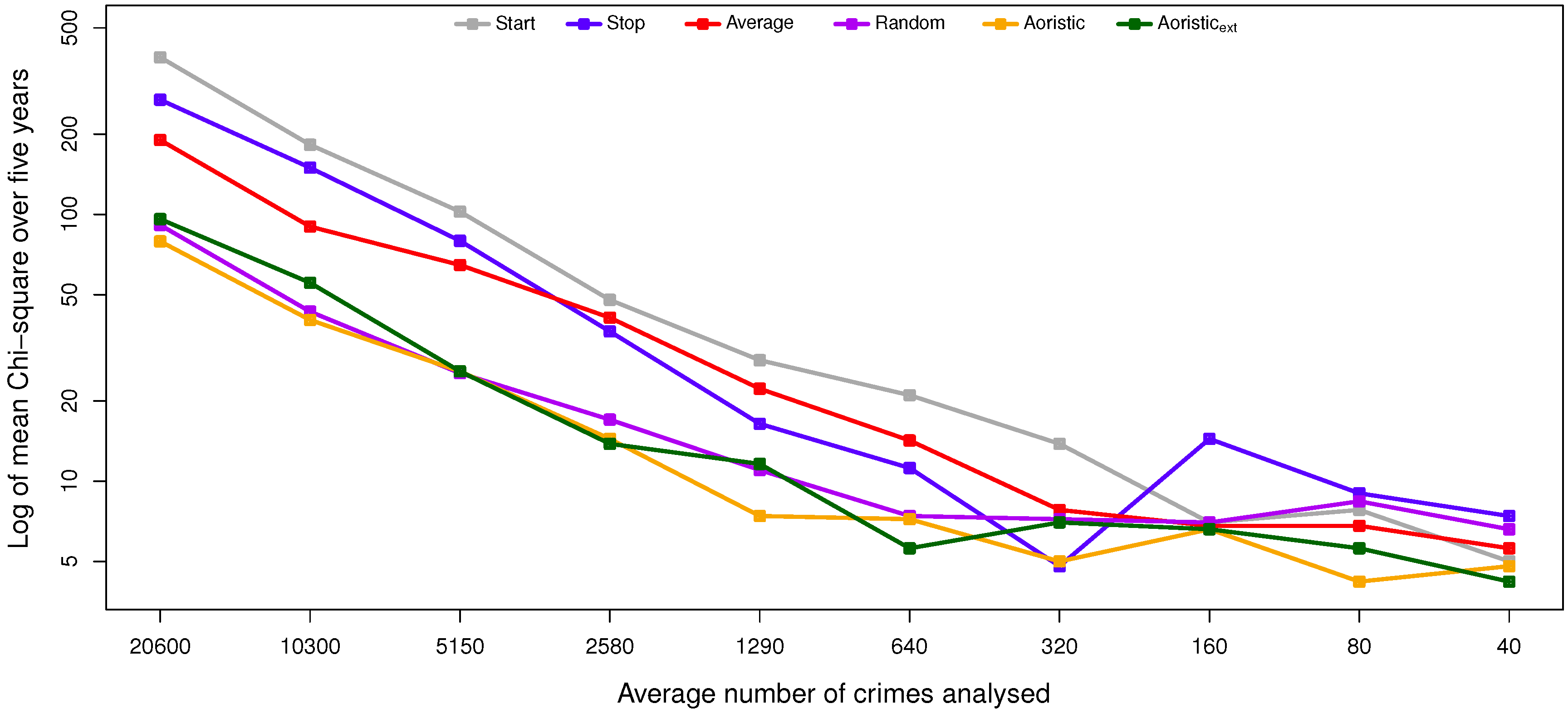
Furthermore, since smaller sample sizes are to be expected in most cases, how a reduction of residential burglary cases affects the accuracy is also investigated in four additional experiments with a two-factor within-subjects design. The additional factor is the dataset that is randomly reduced by 50% ten times, i.e., the factor has ten levels. The result is ten reduced datasets, each including 50% of the burglaries in the previous one. The independent variables are both the candidate methods and the reduced datasets, while the dependent variable is Pearson’s ${\chi }^2$ measure.

In all eight experiments, the temporal methods are evaluated by measuring how well they approximate the ground truth represented as:

• $hou{r}_{actual}$, which is the 24 h of the day with a slot size of $0.5$ h according to Ashby et al. [11], i.e., one day consists of 48 half-hour slots.
• $weekda{y}_{actual}$ that represents the seven days of the week with a slot size of 1 day.
• $mont{h}_{actual}$ that represents the twelve months in a year with a slot size of 1 month.
• $yearda{y}_{actual}$ that represents the 365 days per year, or 366 in leap years, with a slot size of 1 day.

The similarity or divergence between the approximation and actual distribution is measured per year using the evaluation metrics described in Section 5.3. Then, the mean and standard deviation are calculated over the five years for each method. The results are used to suggest which temporal analysis methods are more suitable for determining the temporal distribution of burglaries with regards to the four temporal resolutions.

5.1. Validity Threats

Extracting burglaries with a precisely-known offense time from the dataset and using them for evaluation could potentially be a threat to internal validity. If the extracted subset is not representative of the population of Swedish residential burglaries, there is a risk of biases being introduced. However, this approach has been discussed in previous high-quality research [11]. In addition, domain-experts in the Swedish law enforcement agreed that the assumption that the extracted subset was representative was valid, The reason that some burglaries have known offense times is due to external events, e.g., alarm records, witnesses or the plaintiffs being home during the offense.

Since the data in the present study come from Swedish residential burglaries it is unlikely that the temporal distributions for the four temporal resolutions being investigated could be generalized to other countries. However, since the aim of this work is rather to evaluate the investigated temporal analysis methods’ performance in approximating offense times, this is not an issue.

5.2. Experiment Environment

The residential burglaries’ temporal distributions are produced according to four resolutions. As described in Section 5, the actual distributions are produced based on the burglaries in the dataset for each of the five years individually. Similarly, each methods’ approximate distribution is also produced per year. For each year and representation, the approximate distribution is compared to the actual distribution and the difference measured. For each evaluation measure, the difference between the actual and approximate distribution is averaged over the five years.

The comparison between the methods’ approximation of the ground truth is carried out per year. Since the dataset consists of five years’ worth of burglaries, each distribution is produced per year, resulting in five distributions per resolution, which then are averaged.

5.3. Evaluation Measurement

The performance of the methods is compared against the ground truth, i.e., crime cases with a known exact $offens{e}_{duration}$, using four measurements for comparing distributions: Pearson’s ${\chi }^2$, Euclidean distance, Spearman’s ρ and Kullback–Leibler.

Pearson’s ${\chi }^2$ test is used to compare two sets to investigate the correlation between sets of data. Pearson’s ${\chi }^2$ value should be as small as possible. Since the data used in the experiment are binned, other well-used nonparametric tests, such as Kolmogorov–Smirnov, are not applicable [21]. Therefore, Pearson’s ${\chi }^2$ is used to investigate how well the approximated distribution correlates with the actual distribution. Pearson’s ${\chi }^2$ test, due to its suitability and popularity, will be used as the evaluation measurement for the statistical tests.

The Euclidean distance is used to measure the distance between two distributions, in this case between the actual distributions and the approximations produced by the methods. The Euclidean distance is defined in Equation (6), where $x_i$ and $y_i$ indicate the i-th data point in the respective distribution.

$$d(x,y)=\sqrt{{(x_1-y_1)}^2+{(x_2-y_2)}^2+\dots {(x_n-y_n)}^2}$$

(6)

Spearman’s ρ is a non-parametric rank-based correlation measurement between two variables. The measure ranges between $-1$ and 1, where 0 indicates no correlation between the variables and 1 indicates a positive correlation [22]. The test is used to investigate how well the approximated distribution correlates with the actual distribution.

The Kullback–Leibler divergence is a non-symmetric measure of the information loss when one probability distribution is used for approximating another [23]. It is also known as the information gain, or relative entropy, of one distribution to another. This is measured in the number of extra bits that are required when approximating the first distribution based on the other, i.e., a lower value indicates that two distributions are more similar.

5.4. Statistical Analysis

To evaluate the difference between the methods, the Kruskal-Wallis test is used to investigate whether a significant difference exists between different methods. Kruskal-Wallis is a non-parametric rank-based statistical test for investigating whether two or more samples are from the same distribution [22]. Kruskal-Wallis is used instead of the parametric one-way ANOVA test, as the data were not found to be normally distributed [22]. If a difference exists according to the Kruskal-Wallis test, the Dunn post hoc test is used to investigate between which pairs of methods differences exist. To correct for multiple comparisons, Benjamini-Hochberg adjustment is used [24]. The Benjamini-Hochberg adjustment is used instead of Bonferroni adjustment, as it provides a less restrictive tradeoff with regards to statistical power, although it allows false positives. Additionally, the Benjamini-Hochberg adjustment controls the false discovery rate, whereas the Bonferroni adjustment controls the family-wise error rate.

Further, to evaluate the methods over different sample sizes, Friedman’s test is used. Friedman’s test is a non-parametric two-way analysis of variance [21]. The Nemenyi test is used as a post hoc test to investigate how the methods differ from each other. The Nemenyi test calculates a critical difference (CD) using Tukey’s distribution, and any difference in rank between method pairs that is greater than the CD is considered significantly different [25,26].

5.5. Tools

The crime data were stored in a MySQL relational database. All crime evaluation methods that are evaluated in this work were implemented as scripts in the statistical language R. The scripts make use of the RMySQL, Lubridate and Ggplot2 packages for their internal workings, and they will be available upon request to the corresponding author. Statistical evaluations have used corresponding packages in R.

6. Results

The results are presented and analyzed based on the experimental setup described in Section 5. In Section 6.1, the six methods are evaluated using four different measures to show the correlation and distance between the approximated temporal distribution and the actual temporal distribution. Statistically-significant differences between the methods are also presented. In Section 6.2, the Pearson ${\chi }^2$ results are shown for the methods when the sample size is gradually reduced. Any statistical difference between the methods, using the statistical tests presented in Section 5.4, is also presented.

6.1. Evaluation of the Temporal Analysis Methods on the Full Dataset

Below are the results for the evaluation of the temporal analysis methods using the full dataset and the four different configurations.

6.1.1. Hour Scenario

The mean and standard deviation of the four evaluation measures were calculated for each year from 2010–2014. These can be seen in

Table 4. Mean and standard deviation for the four evaluation measures and six temporal analysis methods that were evaluated with the hour data over each of the five years.

	Pearson’s ${\mathit{\chi }}^{\mathbf{2}}$	Euclidean	Spearman’s ρ	Kullback–Leibler
	(SD)	(SD)	(SD)	(SD)
Start	15720 (2623)	3476 (201)	0.182 (0.14)	0.269 (0.01)
Stop	4982 (1206)	3221 (149)	0.647 (0.13)	0.116 (0.02)
Average	3898 (733)	2980 (144)	0.613 (0.10)	0.068 (0.01)
Random	2055 (581)	2776 (137)	0.605 (0.12)	0.049 (0.02)
Aoristic	1979 (540)	2789 (140)	0.631 (0.12)	0.046 (0.02)
Aoristic${}_{ext}$	1983 (552)	2791 (140)	0.628 (0.12)	0.046 (0.02)

. p-values from the ${\chi }^2$ goodness-of-fit tests were omitted from the results since they were zero, i.e., none of the temporal analysis methods could approximate the baseline distribution in order for the goodness-of-fit tests to consider them being identical. This, however, could be expected since the statistical power of the tests was high due to the large amount of burglaries included in the analysis.

Based on the four evaluation measures presented in Table 4, both the aoristic and aoristic${}_{ext}$ methods performed similarly, although there was a modest advantage for the aoristic method, while the random method performed slightly worse. Average, stop and start performed worse for each of the evaluation measures, except Spearman’s correlation coefficient, which (of the three methods) favored the stop method.

Since statistically significant differences between the methods were found using a Kruskal-Wallis test, ${\chi }^2\left(5\right)=24.5,p=0.000176$, the Dunn post hoc test was used for pair-wise comparisons. The results in

Table 5. Dunn significance test results from pair-wise comparisons between temporal analysis methods over the ${\chi }^2$ hour data.

	Aoristic	Aoristic${}_{\mathit{e}\mathit{x}\mathit{t}}$	Random	Average	Stop	Start
Aoristic
Aoristic${}_{ext}$
Random
Average	*	*
Stop	*	*	*
Start	***	**	**

Critical difference at $p=0.05$:$7.540$, $p=0.01$:$8.900$, $p=0.001$:$10.513$; * Denotes significant difference at $p=0.05$, ** at $p=0.01$, *** at $p=0.001$.

show that both the aoristic and aoristic${}_{ext}$ methods performed significantly better than the average, stop and start methods. The random method performed significantly better than the start and stop methods. Based on these results, it was suggested that the most suitable method for the analysis of hour data was the aoristic method, while the start method was least suitable for the task.

Since the aoristic method was found to be the most suitable method, it was used for plotting the aoristic hour of the day distribution using all burglary data available for the five years. The distribution in Figure 2 is bimodal, or possibly trimodal, with peaks around afternoon and in the night around the early hours. It was clear that the burglary frequency increases during the hours of the day when people are out of their residences as part of their daily routine or during the night when they are at sleep. The baseline, i.e., burglaries with known precise offense time, is shown as a dashed line. It shows a similar bimodal/trimodal distribution, but with a considerably more distinct peak during the night.

6.1.2. Weekday Scenario

Table 6. Mean and standard deviation for the four evaluation measures and six temporal analysis methods that were evaluated with the weekday data over each of the five years.

	Pearson’s ${\mathit{\chi }}^{\mathbf{2}}$	Euclidean	Spearman’s ρ	Kullback–Leibler
	(SD)	(SD)	(SD)	(SD)
Start	383 (102)	7089 (372)	0.798 (0.17)	0.010 (0)
Stop	269 (116)	7022 (358)	0.229 (0.22)	0.006 (0)
Average	190 (55)	7089 (373)	0.683 (0.28)	0.004 (0)
Random	107 (18)	7069 (368)	0.714 (0.24)	0.003 (0)
Aoristic	76 (10)	7065 (361)	0.807 (0.19)	0.002 (0)
Aoristic${}_{ext}$	96 (5)	7068 (365)	0.771 (0.24)	0.002 (0)

includes the mean and standard deviation of the four evaluation measures that were calculated for each year from 2010–2014. Aoristic and aoristic${}_{ext}$ performed similarly on the Euclidean and Kullback–Leibler measures. For Pearson’s ${\chi }^2$ and Spearman’s ρ, there was a more clear advantage for the aoristic method, although aoristic${}_{ext}$ had a considerably smaller standard deviation on the ${\chi }^2$ measure. Compared to the two aoristic methods, the random method performed slightly worse. The average, stop and start methods performed considerably worse for each of the evaluation measures, except Spearman’s ρ, which (of the three methods) favored the start method.

Since statistically-significant differences between the methods were found using a Kruskal–Wallis test, ${\chi }^2\left(5\right)=25.4,p=0.000117$, the Dunn post hoc test was used for pair-wise comparisons. The results in

Table 7. Dunn significance test results from pair-wise comparisons between temporal analysis methods over the ${\chi }^2$ weekday data.

	Aoristic	Aoristic${}_{\mathit{e}\mathit{x}\mathit{t}}$	Random	Average	Stop	Start
Aoristic
Aoristic${}_{ext}$
Random
Average	*
Stop	**	*
Start	***	**	*

Critical difference at $p=0.05$:$7.540$, $p=0.01$:$8.900$, $p=0.001$:$10.513$; * Denotes significant difference at $p=0.05$, ** at $p=0.01$, *** at $p=0.001$.

show that the aoristic method performed significantly better than the average, stop and start methods, while the aoristic${}_{ext}$ method performed significantly better than the two latter. The random method performed significantly better than the start method. Based on these results, it was suggested that the most suitable method for the analysis of weekday data was the aoristic method, while the start method was least suitable.

Since the aoristic method was found to be the most suitable method, it was used for plotting the aoristic weekday distribution using all burglary data available for the five years. As shown in Figure 3, there are peaks during Fridays and Saturdays and a considerable drop on Sundays. The peaks can be explained by that people usually go on recreational activities during the weekends, leaving their homes unguarded. The drop on Sundays is harder to explain, but it might be due to burglars also using Sundays for recreation. Law enforcement officers have speculated that Sundays are when stolen goods most often are fenced. In Figure 3, the baseline, i.e., burglaries with a known precise offense time, is shown as a dashed line. It shows a similar distribution, but with a less distinct peak during Fridays and Saturdays.

6.1.3. Month Scenario

Table 8. Mean and standard deviation for the four evaluation measures and the six temporal analysis methods that were evaluated with the month data over each of the five years.

	Pearson’s ${\mathit{\chi }}^{\mathbf{2}}$	Euclidean	Spearman’s ρ	Kullback–Leibler
	(SD)	(SD)	(SD)	(SD)
Start	10.24 (1.9)	313.4 (37)	0.978 (0.02)	2.542$\times {10}^{-4}$ (0)
Stop	10.68 (3.3)	389.2 (47)	0.974 (0.02)	2.535$\times {10}^{-4}$ (0)
Average	6.74 (2.2)	326.4 (38)	0.980 (0.02)	1.664$\times {10}^{-4}$ (0)
Random	6.34 (1.4)	326.2 (37)	0.982 (0.02)	1.574$\times {10}^{-4}$ (0)
Aoristic	3.19 (0.5)	377.2 (46)	0.991 (0.01)	7.705$\times {10}^{-5}$ (0)
Aoristic${}_{ext}$	3.22 (0.5)	386.8 (48)	0.991 (0.01)	7.792$\times {10}^{-5}$ (0)

includes the mean and standard deviation of the four evaluation measures that were calculated for each year from 2010–2014. As can be seen, the ${\chi }^2$ and Euclidean measures are considerably lower compared to the hour of the day and day of the week resolutions. This is because there is less monthly variation of burglaries compared to variation over half-hours or weekdays. In fact, merely 6% of the burglaries have start and end dates in different months compared to 39% and 83% that have start and end dates in different days and half-hours, respectively.

Both the aoristic methods performed similarly and showed the best performance with regards to the evaluation measures, except for the Euclidean distance, which instead was in favor for the start, random and average methods. Random and average also performed similar to each other and were next best out of the six methods, while start and stop performed worst, taking all measures into account. Based on these results, it was suggested that the most suitable method for the analysis of month data was the aoristic method, while the stop method was least suitable for the task. However, no statistically-significant differences were found between the six methods using a Kruskal–Wallis test, ${\chi }^2\left(5\right)=0.38,p=0.996$.

Since the aoristic method is suggested to be the most suitable method based on the results, and for consistency between the subsections, it was used for plotting the aoristic month distribution for the full five-year burglary data. The distribution in Figure 4 shows peaks during the autumn and winter months that usually is explained by darker days, due to daylight saving time, allowing burglars to move around unnoticed to a larger extent. There is also a slight peak in July, which is the biggest vacation month in Sweden.

6.1.4. Day in Year Scenario

Table 9. Mean and standard deviation for the four evaluation measures and the six temporal analysis methods that were evaluated with the day of year data over each of the five years.

	Pearson’s ${\mathit{\chi }}^{\mathbf{2}}$	Euclidean	Spearman’s ρ	Kullback–Leibler
	(SD)	(SD)	(SD)	(SD)
Start	5761 (556)	1020 (53)	0.416 (0.03)	0.103 (0.01)
Stop	5721 (405)	1006 (51)	0.428 (0.03)	0.092 (0.01)
Average	5479 (405)	1010 (52)	0.455 (0.03)	0.091 (0.01)
Random	5367 (402)	1006 (51)	0.458 (0.04)	0.090 (0.01)
Aoristic	5187 (465)	1003 (51)	0.478 (0.03)	0.087 (0.01)
Aoristic${}_{ext}$	5231 (416)	1004 (51)	0.476 (0.03)	0.087 (0.01)

includes the mean and standard deviation of the four evaluation measures that were calculated for each year from 2010–2014 in the day in year temporal resolution. Both aoristic methods show promising results, with a slight advantage for the aoristic method. The differences between all six methods are smaller than in the previous configurations. As a consequence, no statistically-significant differences were found between the methods using a Kruskal–Wallis test, ${\chi }^2\left(5\right)=1.30,p=0.930$.

Since the aoristic method showed the most promising results, it was used for plotting the aoristic day of the year distribution based on the full five-year burglary data. The most distinct peak in the distribution shown in Figure 5 is on Christmas Eve, which is celebrated on the 24^th of December in Sweden. This contradicts the results by Cohn and Rotton that burglaries are under-represented during Christmas in a U.S. setting [19]. Other peaks are during November and December, including 1 January, related to New Year’s eve. The lowest burglary frequency, if disregarding the leap day 29 February, was recorded on the last of December.

6.2. Evaluation of Temporal Analysis Methods on Reduced Data

Below are the results for the evaluation of the temporal analysis methods using the reduced dataset (samples of the full dataset) and the four different configurations.

6.2.1. Reduced Hour Scenario

The results in Figure 6 indicate that both aoristic methods show the lowest ${\chi }^2$ measure as the number of burglaries being analyzed is reduced. As long as there are more than roughly 10,000 burglaries, the random method performs close to the aoristic methods. Then, as the numbers of burglaries are reduced, the random method shows decreasing performance due to the law of large numbers. When analyzing crimes in the hundreds, the aoristic methods are clearly most suitable for the task at hand. If analyzing around 40–100 crimes, the difference in performance is substantial between the aoristic methods, on the one hand, and the random, stop and average methods, on the other hand, were the latter three show very similar performance. The start method is the worst alternative throughout the whole range.

The Friedman test found that there exist statistical differences between the analysis methods, ${\chi }^2\left(9\right)=53.709,p=2.144*{10}^{-8}$. Since statistical differences were found, a Nemenyi post hoc test was used for pair-wise comparisons between methods. As shown in

Table 10. Nemenyi significance test results from pair-wise comparisons between temporal analysis methods in the temporal resolutions of hour in the day with reduced number of available crimes during analysis.

	Aoristic	Aoristic${}_{\mathit{e}\mathit{x}\mathit{t}}$	Random	Average	Stop	Start
Aoristic
Aoristic${}_{ext}$
Random
Average	*	*
Stop	**	**
Start	***	***	*
Average rank	1.40	1.60	3.20	4.20	4.60	6.00

Critical difference at $p=0.05$:$2.384$, $p=0.01$:$2.814$, $p=0.001$:$3.324$; * Denotes significant difference at $p=0.05$, ** at $p=0.01$, *** at $p=0.001$.

, both aoristic methods were significantly better than the average, stop and start methods, while random was significantly better than start. The average ranks from the Friedman test are also shown in Table 10, and the aoristic method receives the best ranks, followed by aoristic${}_{ext}$.

6.2.2. Reduced Weekday Scenario

The results in Figure 7 indicate that both aoristic methods show the lowest ${\chi }^2$ all together. When roughly 320 crimes are being analyzed, the stop method suddenly receives the best ${\chi }^2$ measure, but when 160 crimes are being analyzed, the stop method is the worst candidate. Overall, the aoristic method was the best candidate for estimating weekday crime frequencies throughout the range sizes.

The Friedman test found that there exist statistical differences between the analysis methods, ${\chi }^2\left(9\right)=50.529,p=8.564\times {10}^{-8}$. A Nemenyi post hoc test revealed that the aoristic method was significantly better than average, stop and start, while aoristic${}_{ext}$ dominated the stop and start methods; see

Table 11. Nemenyi significance test results from pair-wise comparisons between temporal analysis methods in the temporal resolutions of weekday with reduced numbers of crimes available during analysis.

	Aoristic	Aoristic${}_{\mathit{e}\mathit{x}\mathit{t}}$	Random	Average	Stop	Start
Aoristic
Aoristic${}_{ext}$
Random
Average	*
Stop	**	*
Start	***	**
Average rank	1.60	2.10	3.15	4.20	4.60	5.35

Critical difference at $p=0.05$:$2.384$, $p=0.01$:$2.814$, $p=0.001$:$3.324$; * Denotes significant difference at $p=0.05$, ** at $p=0.01$, *** at $p=0.001$.

. The average ranks from the Friedman test suggest that the aoristic method is the most suitable method for analyzing weekday crime frequencies.

6.2.3. Reduced Month Scenario

As shown in Figure 8, the six temporal analysis methods performance fluctuate throughout the whole range of numbers of crimes when estimating the monthly crime distribution. It is hypothesized that the fluctuation is because of the low ${\chi }^2$ measure received in the month resolution due to relative small variance, 6%, compared to the day of the week and hour of the day resolutions with 39% and 83%, respectively. However, the overall trend with declining numbers of mean ${\chi }^2$ measures that stabilize around 300 crimes is similar to the precious temporal resolutions of hours in the day and weekday. It is hard to extract any method as better or worse than any other method only by looking at Figure 8. Therefore, a Friedman test was executed, which revealed that there exist differences between the six methods and/or the ten datasets, ${\chi }^2\left(9\right)=50.42,p=8.98\times {10}^{-8}$.

Unfortunately, the Nemenyi post hoc test could not identify any statistically-significant differences between the six temporal analysis methods. The average ranks of the temporal analysis methods over the datasets are presented in

Table 12. Average ranks of the six temporal analysis methods in the temporal resolution of month in the year and with reduced numbers of crimes available during analysis. A lower rank is favorable.

	Aoristic	Aoristic${}_{\mathit{e}\mathit{x}\mathit{t}}$	Random	Average	Stop	Start
Average rank	2.55	3.05	3.65	3.70	3.85	4.20

Critical difference at $p=0.05:2.384$, $p=0.01$:$2.814$, $p=0.001$:$3.324$.

showing that the aoristic method has lowest rank, which indicates that it is the most suitable candidate method for estimating monthly temporal crime distributions.

6.2.4. Reduced Day in Year Scenario

Figure 8 shows the performance for the six methods when estimating the crime frequency per day in a year as the number of crimes included in the analysis declines. Five of the methods had a similar declining trend as the previous configurations investigated that stabilize around 300 crimes. However, the average method shows inferior performance in estimating the crime frequency in the day of year configuration. Due to its extreme behavior, the correctness of the average method implementation was re-tested, but no errors were found. A Friedman test revealed that statistical differences existed between the six methods and/or datasets, ${\chi }^2\left(9\right)=23.709,p=0.00479$.

A Nemenyi post hoc test identified that aoristic${}_{ext}$ dominated the average, start and stop methods, while the aoristic method outperformed the average and start methods; see

Table 13. Nemenyi significance test results from pair-wise comparisons between temporal analysis methods in the temporal resolution of day in year and with reduced numbers of crimes available during analysis.

	Aoristic	Aoristic${}_{\mathit{e}\mathit{x}\mathit{t}}$	Random	Average	Stop	Start
Aoristic
Aoristic${}_{ext}$
Random
Average	***	***	**
Stop		**
Start	*	***
Average rank	2.10	1.10	2.80	5.80	4.40	4.80

Critical difference at $p=0.05$:$2.384$, $p=0.01$:$2.814$, $p=0.001$:$3.324$; * Denotes significant difference at $p=0.05$, ** at $p=0.01$, *** at $p=0.001$.

. The random method also performed significantly better than the average method. The average ranks from the Friedman test suggest that the aoristic${}_{ext}$ method was the best candidate for estimating the crime frequency in the day of year resolution.

7. Analysis and Discussion

Today, law enforcement uses an ad hoc approach to estimating the temporal distribution of residential burglaries. This approach could influence resource planning negatively, as it is difficult to predict how crimes distributions will change over time. Often, experience is prevalent in the decision making process. In this paper, multiple approaches for estimating an approximate temporal distribution of residential burglaries have been investigated.

A method that is able to approximate the temporal distribution of crimes is a key component, together with spatial data, when for instance, law enforcement agencies schedule patrols and other resources more efficiently to better be in sync when crimes actually occur. For example, having a set of hourly approximations that corresponds well to the actual temporal distributions of residential burglaries in different areas of a municipality allows patrols to be present in the correct area when there is a higher likelihood of a residential burglary taking place, i.e., a prioritization of the patrol route.

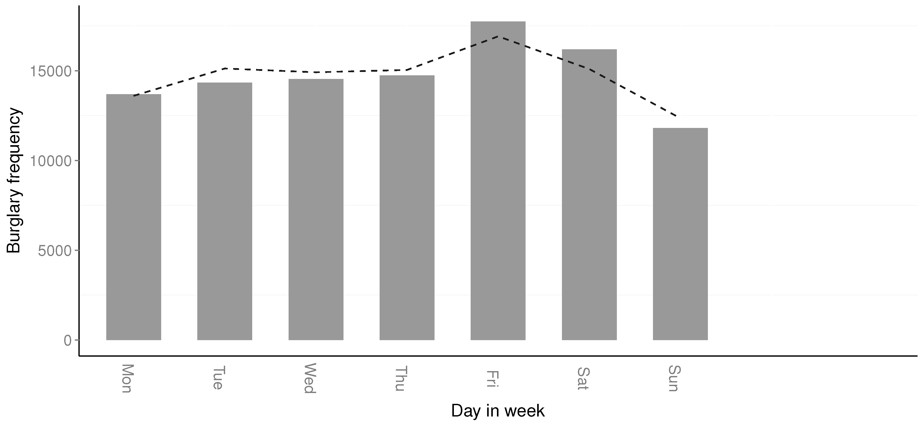
By approximating the temporal distribution of residential burglaries over days in the week allows law enforcement administration to better schedule law enforcement officers for different tasks. The temporal distribution regarding weekdays in Table 3 suggests that there is a spike in residential burglaries on Fridays and Saturdays, to then decrease on Sundays. This suggests that it is more efficient to have law enforcement officers focus on residential burglaries on Fridays and Saturdays, than on Sundays. 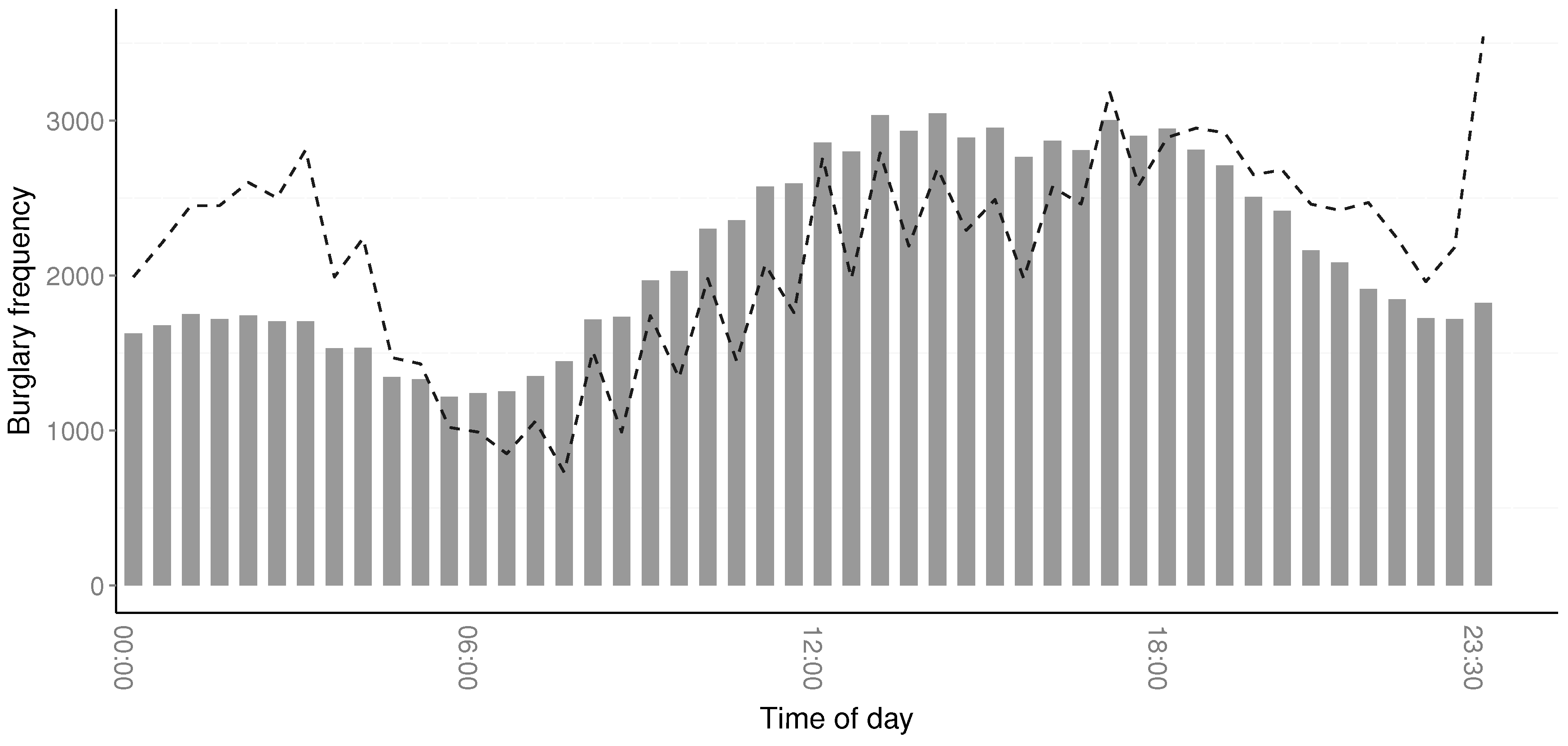Further, Table 2 suggests that most residential burglaries take place during working hours. Having an analysis on different geographical areas and specific days would allow law enforcement to further distinguish patterns in the data.

Looking at the actual distributions, the data suggest that $21.9\%$ burglaries are committed during a span of at least one hour; $43.7\%$ of the residential burglaries occur within six hours. As time increases, the amount of burglaries that span long segments is decreasing; $26.7\%$ of crimes are committed during a time period of more than one day, i.e., the crime could have been committed during that time span; only $6.8\%$ of the residential burglaries are committed sometime during a time span of more than one week, which means crimes can go unreported for a long time. In the data, $6.8\%$ represent an absolute number of 7009 burglaries over five years. That is quite a large number of burglaries that is unreported for a long time. It can be noted, however, that most crimes occur within a six-hour time span. As such, being able to detect changes in trends requires the ability to determine the distribution on an hourly resolution. If the estimation of the crime distribution only occurs on a longer time span, the details will be lost. This puts further emphasis on the need to accurately estimate the crime distribution on an hourly scale [13].

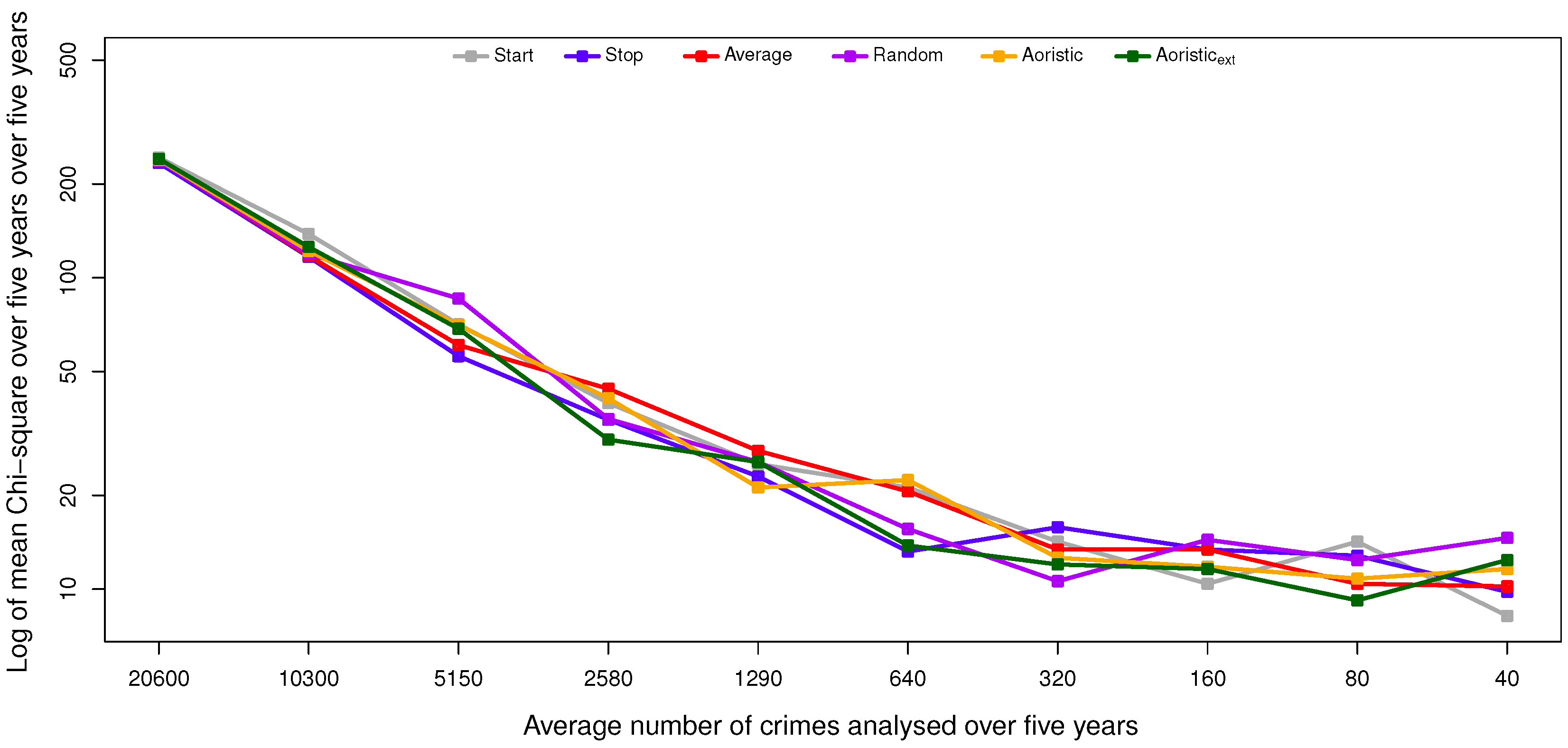
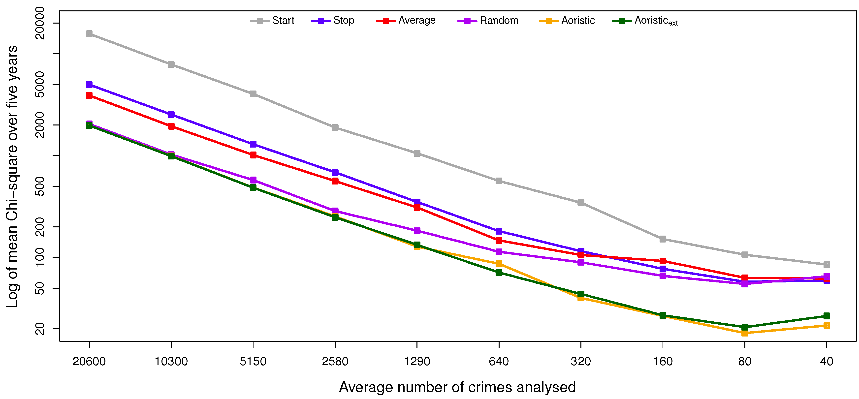
The results and the statistical analysis suggest that the aoristic and aoristic${}_{ext}$ methods are preferred over the other methods for estimating the temporal distribution of residential burglaries, as they perform significantly better than the stop, average and start method in multiple configurations. The aoristic${}_{ext}$ method is quite complex compared to the aoristic method, and it does not suggest improved results when compared to the aoristic method. We hypothesize that this is due to limited detail in the temporal data to support the aoristic${}_{ext}$ method, e.g., because both plaintiffs and witnesses could round off the time of their observations to structured time units, such as quarters, half-hours or even whole hours. That way, the temporal resolution in the data is decreased.

However, when the temporal resolution is instead unique days in the year, such subtle differences have a negligible effect. In that particular case, the aoristic${}_{ext}$ method also comes out as the most suitable candidate, but interestingly, this does not apply when estimating the day in the week or month in the year. Those deviations could depend on the rather low granularity in those cases, i.e., seven and 12 slots, respectively. In the end, both aoristic methods produce usable results; the trade-off is one between accuracy and time complexity, i.e., execution times, given that temporal data with sufficient resolution exist. If the main focus is on time complexity, then a random method that, rather than a uniform distribution, instead uses the distribution of crimes with known offense time would probably render usable results as long as sufficiently many crimes are included in the analysis.

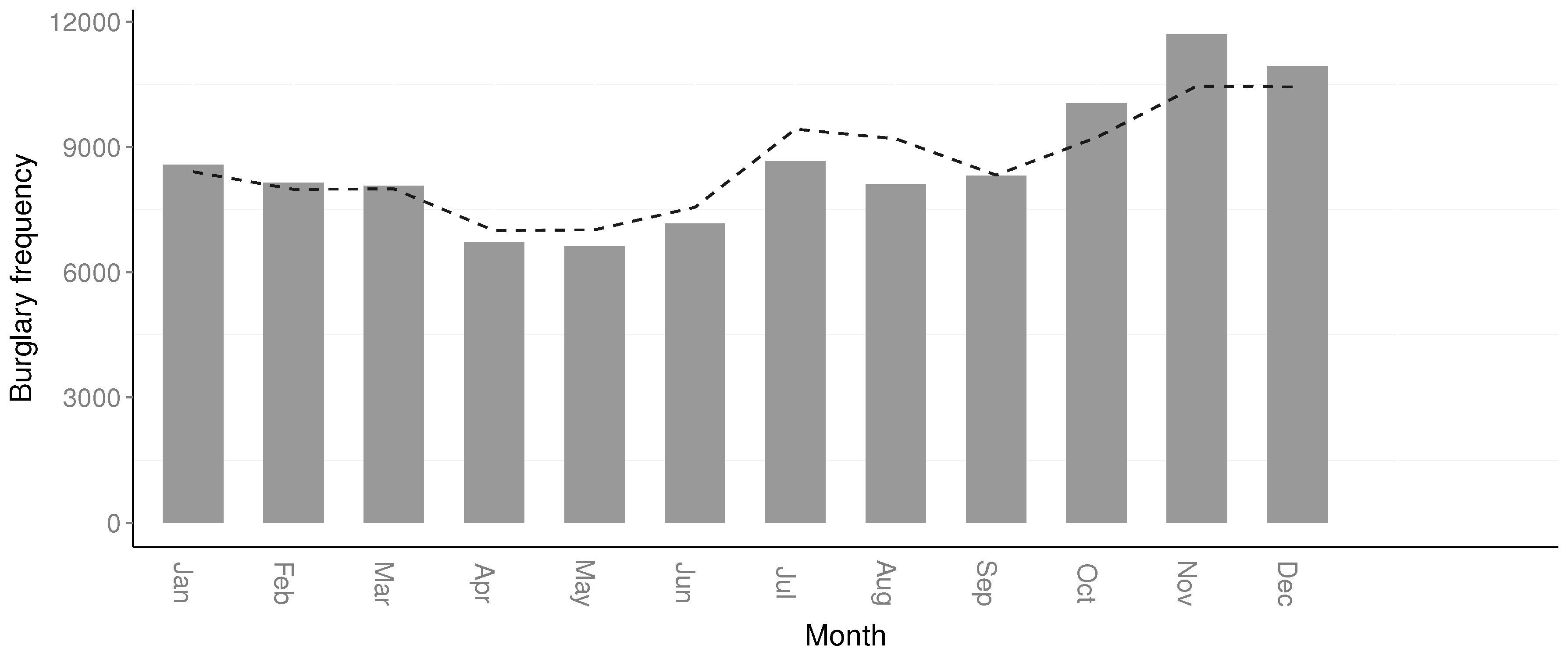
The scenarios with a reduced number of crimes included in this study are important, as in practice, smaller sample sizes are more likely. Further, by having large sample sizes, it is more likely that various trends or other variables are “smoothed”. This is a concern for, e.g., the hour, day in week, and month resolutions, as seasonal changes might impact the trend in the short term [19]. Smaller timescales will be more successful in providing short-term forecasts. However, as the goal of this study was to identify the algorithm most efficient at approximating the temporal distribution, this is not deemed problematic. Even with a reduced dataset, the findings still hold.

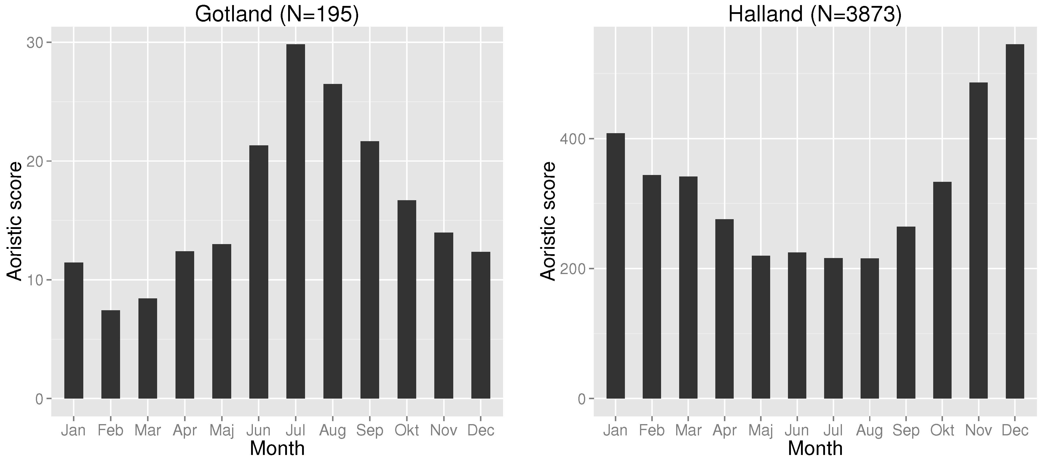
While a smaller temporal window is likely to be preferred for temporal forecasting, a smaller geographical area is likewise more likely to improve results. Criminals operate under different constraint in different geographical areas and affect the temporal distribution. Further, seasonal changes affect regions and crime opportunities differently, e.g., in vacation areas. This also allows different areas to be forecast differently and, as such, might further optimize resource scheduling. An initial study showed that the temporal distribution for the Swedish county of Halland differed quite a bit from the county of Gotland; see Figure 9. During the summer, residential burglaries decreased in Halland, but increased in Gotland due to vast numbers of tourists visiting the island. While it might be argued that the geographical division at this level is still too large, the differences are still visible.

Estimating the temporal distributions and using in forecasting crime trends would allow an administrative overview enabling the simplification of resource scheduling. For example, extra patrols might be present during Friday and Saturday evenings in residential areas or weekday evenings have a lower amount of patrols in residential areas. The temporal distribution allows law enforcement agencies to, based on knowledge of when crimes most likely occur, schedule their personnel and determine when targeted measures could result in optimal effect.

The data used in this study have minute precision for the start and end of time spans, i.e., a crime occurrence time can span between, for instance, 10:29–14:53. However, in $54.5\%$ of burglaries, the start time is reported with an hour precision, while this is true for $3.4\%$ of end times. Most likely, this is due to uncertainties of when the crime started and the reported time being rounded to the closest hour. The lack of precision in the data is most likely why the results for the aoristic${}_{ext}$ method are not better than the aoristic method. The lack of precision in reported time span, together with the longer time spans, drown out any improvement that the aoristic${}_{ext}$ method offers against the aoristic method.

Limitations

While the aoristic${}_{ext}$ method extends the aoristic method with a level of complexity that has the possibility of increasing the precision of the estimated time, it also requires a more precise data collection, i.e., the time span collected must be more precise, for both the start and end time. If the collected crime information only states that the crime occurred between 13 and 16 on a given day, the aoristic${}_{ext}$ method will not be better than the aoristic method. In that case, the aoristic${}_{ext}$ should fall back to the aoristic method’s relatively simpler approach. The same holds for time spans where either the start or the end time is not precise enough. In that case, the point distribution will be similar to the aoristic method (given that the time span exceeds a certain number of time units). However, if the collected temporal information, in the span, contains minutes, the precision is potentially improved. This is reasonable, as Table 3 suggests that a majority of the crimes (>50%) has a reported time span of less than twelve hours.

For longer time spans, there is less likelihood that the data are collected with such precision that the aoristic${}_{ext}$ will yield improved results. Further, with longer time spans, the lower resolution will have less impact, as the points affect the final distribution to a lesser extent (points are more spread out). The same is true for the aoristic method, as well.

8. Conclusions

Crime analysis requires precise temporal information. In many cases, the temporal information is uncertain or available as a time span. Consequently, approximating offense times of crimes that often lack precise time information is important. In an experiment, the accuracy of six temporal analysis methods, five existing and one novel, was evaluated regarding their ability to approximate offense times.

The results indicate that the aoristic and aoristic${}_{ext}$ methods performed significantly better than the average, start and stop methods. However, the novel aoristic${}_{ext}$ method was not significantly better than the aoristic method. The aoristic${}_{ext}$ method does in the worst case scenario behave similar to the aoristic method. Given a certain level of precision in the collected data, the estimated time for crimes will be more precise. However, if such a level of precision in the estimated time is not needed, the added complexity of the aoristic${}_{ext}$ method does not justify its use over the aoristic method.

For future work, a simulation-based evaluation of temporal analysis methods using another dataset would be interesting to carry out as a complement to the present study. It would also be interesting to investigate if small sample sizes on specific geographic areas would suggest whether the results still hold for, e.g., a specific city or different areas of a city. Further, investigating whether temporal distributions for different geographic areas affect each other and if methods can be developed to estimate links between geographically-limited distributions automatically. This would allow law enforcement to observe how residential burglary trends move across geographic areas.

References

1. Ratcliffe, J.H. Aoristic signatures and the spatio-temporal analysis of high volume crime patterns. J. Quant. Crim. 2002, 18, 23–43. [Google Scholar] [CrossRef]
2. Santos, R.B. Crime Analysis with Crime Mapping, 3rd ed.; SAGE Publications: Thousand Oaks, CA, USA, 2013. [Google Scholar]
3. Chainey, S.; Ratcliffe, J. GIS and Crime Mapping; John Wiley & Sons: Hoboken, NJ, USA, 2005. [Google Scholar]
4. Perry, W.L.; McInnis, B.; Price, C.C.; Smith, S.; Hollywood, J.S. Predictive Policing; RAND Corporation: Santa Monica, CA, USA, 2013. [Google Scholar]
5. Rey, S.J.; Mack, E.A.; Koschinsky, J. Exploratory space-time analysis of burglary patterns. J. Quant. Crim. 2011, 28, 509–531. [Google Scholar] [CrossRef]
6. Leitner, M.; Helbich, M. The impact of hurricanes on crime: A spatio-temporal analysis in the city of Houston, texas. Cartogr. Geogr. Inf. Sci. 2013, 38, 213–221. [Google Scholar] [CrossRef]
7. Brantingham, P.J.; Brantingham, P.L. Environmental Criminology, 2nd ed.; Waveland Press: Long Grove, IL, USA, 1991. [Google Scholar]
8. Johnson, S.D.; Bernasco, W.; Bowers, K.J.; Elffers, H.; Ratcliffe, J.; Rengert, G.; Townsley, M. Space-Time patterns of risk: A cross national assessment of residential burglary victimization. J. Quant. Criminol. 2007, 23, 201–219. [Google Scholar] [CrossRef]
9. Iwanski, N.; Frank, R.; Dabbaghian, V.; Reid, A.; Brantingham, P. Analyzing an offender’s journey to crime: A criminal covement model (CriMM). In Proceedings of the European Intelligence and Security Informatics Conference, Athens, Greece, 12–14 September 2011.
10. Ratcliffe, J.H. A temporal constraint theory to explain opportunity-based spatial offending patterns. J. Res. Crime Delinq. 2006, 43, 261–291. [Google Scholar] [CrossRef]
11. Ashby, M.P.; Bowers, K.J. A comparison of methods for temporal analysis of aoristic crime. Crime Sci. 2013, 2, 1–16. [Google Scholar] [CrossRef]
12. Ratcliffe, J.H.; McCullagh, M.J. Aoristic crime analysis. Int. J. Geogr. Inf. Sci. 1998, 12, 751–764. [Google Scholar] [CrossRef]
13. Felson, M.; Poulsen, E. Simple indicators of crime by time of day. Int. J. Forecast. 2003, 19, 595–601. [Google Scholar] [CrossRef]
14. Tompson, L.; Townsley, M. (Looking) Back to the future: Using space-time patterns to better predict the location of street crime. Int. J. Police Sci. Manag. 2012, 12, 23–40. [Google Scholar] [CrossRef]
15. Vasiliev, I.R. Mapping time. Cartographica: Int. J. Geogr. Inf. Geovis. 2006, 34, 1–51. [Google Scholar] [CrossRef]
16. Ratcliffe, J.H. Aoristic analysis: The spatial interpretation of unspecific temporal events. Int. J. Geogr. Inf. Sci. 2000, 14, 669–679. [Google Scholar] [CrossRef]
17. Cohen, L.E.; Felson, M. Social change and crime rate trends: A routine activity approach. Am. Soc. Rev. 1995, 44, 588–608. [Google Scholar] [CrossRef]
18. Rotton, J.; Frey, J. Air pollution, weather, and violent crimes. J. Person. Soc. Psychol. 1985, 49, 1207–1220. [Google Scholar] [CrossRef]
19. Cohn, E.G.; Rotton, J. Even criminals take a holiday: Instrumental and expressive crimes on major and minor holidays. J. Crim. Justice 2003, 31, 351–360. [Google Scholar] [CrossRef]
20. Brunsdon, C.; Corcoran, J. Using circular statistics to analyse time patterns in crime incidence. Com. Environ. Urban Syst. 2006, 30, 300–319. [Google Scholar] [CrossRef]
21. Kvam, P.H.; Vidakovic, B. Nonparametric statistics with applications to science and engineering. In Wiley Series in Probability and Statistics; John Wiley & Sons: Hoboken, NJ, USA, 2007. [Google Scholar]
22. Sheskin, D.J. Handbook of Parametric and Nonparametric Statistical Procedures, 5th ed.; CRC: Boca Raton, FL, USA, 2011. [Google Scholar]
23. Bickel, P.J.; Doksum, K.A. Mathematical Statistics 2e, 2nd ed.; Prentice Hall: Upper Saddle River, NJ, USA, 2006. [Google Scholar]
24. Benjamini, Y.; Hochberg, Y. Controlling the false discovery rate: A practical and powerful approach to multiple testing. J. R. Stat. Soc. 1995, 57, 289–300. [Google Scholar]
25. Demsar, J. Statistical comparisons of classifiers over multiple data sets. J. Mach. Learn. Res. 2006, 7, 1–30. [Google Scholar]
26. Hollander, M.; Wolfe, D.A.; Chicken, E. Nonparametric Statistical Methods; John Wiley & Sons: Hoboken, NJ, USA, 1999. [Google Scholar]
Figure 1. (a) The aoristic score for an example offense spanning four hours according to the time span of 20:45–23:10; (b) The aoristic e x t scores for the same example.
Ijgi 05 00148 g001
Figure 2. Aoristic distribution of all burglaries and attempted burglaries with an hour resolution between 2010 and 2014 with the baseline shown as a dashed line.
Ijgi 05 00148 g002
Figure 3. Aoristic distribution of all burglaries and attempted burglaries with the day in the week resolution between 2010 and 2014 with the baseline shown as a dashed line.
Ijgi 05 00148 g003
Figure 4. Aoristic distribution of all burglaries and attempted burglaries with a month resolution between 2010 and 2014 with the baseline shown as a dashed line.
Ijgi 05 00148 g004
Figure 5. Aoristic distribution of all burglaries and attempted burglaries with a day in the year resolution between 2010 and 2014 with the baseline shown as a dashed line. A rolling window mean of four days was applied to the baseline to increase readability.
Ijgi 05 00148 g005
Figure 6. Development of each analysis method with regards to Pearson’s χ 2 measure of the hour distributions as crimes are repeatedly reduced by 50%. The plot is based on all Swedish burglaries between 2010 and 2014 (N = 103,029).
Ijgi 05 00148 g006
Figure 7. Development of each analysis method with regards to Pearson’s χ 2 measure of the weekday distributions as crimes are repeatedly reduced by 50%. The plot is based on all Swedish burglaries between 2010 and 2014 (N = 103,029).
Ijgi 05 00148 g007
Figure 8. Development of each analysis method with regards to Pearson’s χ 2 measure of the month distributions as crimes are repeatedly reduced by 50%. The plot is based on all Swedish burglaries between 2010 and 2014 (N = 103,029).
Ijgi 05 00148 g008
Figure 9. Aoristic crime frequency distribution per month based on five years’ worth of residential burglaries in two different counties in Sweden.
Ijgi 05 00148 g009