Measuring Land Take: Usability of National Topographic Databases as Input for Land Use Change Analysis: A Case Study from Germany

Abstract

The implementation of sustainable land policies is in need of monitoring methods that go beyond a mere description of the proportion values of land use classes. The annual statistical surface area report on actual land utilization (German: “Bodenfläche nach Art der tatsächlichen Nutzung”), published by the statistical offices of the German federal states and the federation, provides information on a set of pre-defined land use classes for municipalities, districts and federal states. Due to its surveying method of summing up usage information from cadastral registers, it is not possible to determine previous and subsequent usages of land parcels. Hence, it is hard to precisely indicate to what extent particular land use classes contribute to the settlement area increase. Nevertheless, this information is crucial to the understanding of land use change processes, which is needed for a subsequent identification of driving forces. To overcome this lack of information, a method for the spatial and quantitative determination of previous and subsequent land usages has been developed, implemented and tested. It is based on pre-processed land use data for different time slices, which are derived from authoritative geo-topographical base data. The developed method allows for the identification of land use changes considering small geometric shifts and changes in the underlying data model, which can be adaptively excluded from the balance.

1. Introduction

In developed countries, an ongoing increase of land take for settlement and transportation infrastructures can be observed [1,2,3,4]. Thus, despite a stagnating or even shrinking population, cities demand for new construction areas, which lead to an increase of urban sprawl [5,6]. As a consequence, ecologically-valuable areas in the surrounding of cities are in danger of being converted into settlement or transportation infrastructures.

In Germany, the amount of land that was converted from open space into settlement or traffic usages was about 298 km² in the year 2014, which is about 0.08% of the country. This number is based on the official land use statistics published by the Federal statistical office [7] and calculates to a daily settlement land take of about 74 hectares in a four-year average [8]. In the national Sustainable Strategy, the German government stated the political will to limit this amount to a value of 30 hectares per day by 2020 (the so-called “30-ha-goal”) [9]. Hence, land use monitoring and area requirement projections are becoming more and more important in order to identify the driving forces for land take and to ensure sustainability in urban development [10].

However, it is hard to get reliable results for the measurement of the real land use change since the changes to be measured are small in relation to the accuracy that can be obtained from the statistical surveys that are currently available. Since spatial planning in Germany is up to the federal states and the communes, the national 30-ha-goal has to be broken down to lower administrative levels since “federal states and municipalities are responsible for implementing appropriate measures in practice” to achieve land take reduction goals (cf. [11]). In this regard, the quality of the input data with respect to topicality, accuracy, reliability and validity is crucial for land use change detection. Desirably, this monitoring should be based not only on the comparison of land use proportions, but also show the evidence of the actual usage conversion of land parcels [12].

In this study, we propose a method to determine land use changes based on authoritative geo-topographical base data from different time slices. By comparing previous and subsequent land use information of the datasets, it is possible to spatially identify specific land use categories that are more or less affected by land conversion. Therefore, it will be possible to analyze the spatial effects of urbanization by localizing hot-spots of land take, which is defined as part of the EEA core set of indicators (CSI) [13].

2. Materials and Methods

2.1. Input Data

2.1.1. Database Requirements

Land use data collection and analyzing is performed worldwide on global, regional and local levels and is based on many different input datasets and methods. Depending on the mapping scale, a number of input data can be accounted for the delivery of sufficient land use information.

As shown above, small-scale approaches of land use change monitoring of spacious areas like continents or sub-continental regions have limitations regarding the effects caused by patches smaller than the defined MMU. However, the totality of single construction operations (e.g., housing area development, road construction) has considerable impacts.

Therefore, the following criteria for land use monitoring input data can be stated, especially in the context of the settlement development [14]:

• Exhaustive availability: The dataset must cover the complete area under investigation. In case of a national monitoring, all municipalities of a country must be recorded.
• Homogeneous data structure: The dataset must be uniformly structured throughout the complete area in order to ensure comparability for the geometry, as well as for the attribute data.
• Updating guarantee: The input data must be updated regularly and with an unlimited temporal horizon. The data acquisition methods should be as constant as possible over the updating cycles to ensure consistent time series.
• Sufficient spatial resolution: The geographical input data must provide an adequate surveying scale to reproduce the settlement development in the desired granularity.
• Optional linkage of the base data with specific geographical and statistical data: The input data must offer the possibility for joining specific information originating from any spatially-related environmental, geographical, socio-economical or statistical data. The spatial relation should be possible by overlapping geometrical datasets, as well as by employing unambiguous keys.

2.1.2. International Datasets

There are several land use monitoring programs on the national and international levels. CORINE Land Cover (CLC) has been widely used for numerous studies. It is also used for the land take indicator measurement of the European Environment Agency [15]. The suitability of CLC data for a consistent land use change monitoring is limited due to the long repeating intervals (1990, 2000, 2006, 2012), the changing data sources for the mapping process (different remote sensing platforms) and the limited spatial resolution with MMUs of 25 ha and 5 ha for land use changes [16,17,18].

Urban Atlas as part of the Copernicus Land Monitoring Services project provides land use data for nearly all European cities (or urban agglomerations) of more than 50,000 inhabitants. The MMU of Urban Atlas is 0.25 ha for urban land use classes and has a very high granularity with respect to CLC data. However, the second time slice of Urban Atlas is currently not yet validated, and therefore, urban monitoring on that basis has some uncertainties. Additionally, for the population threshold, there is no information for rural or micropolis areas from this dataset [19].

Therefore, these datasets have their advantages for international comparative studies on city areas. However, on a national or regional level, they are not suitable for a high-resolution and area-covering monitoring of land use. A comparative study that analyzed different datasets regarding their potential of monitoring land use change revealed significant differences in their suitability for regional and national land take measurements [20].

2.1.3. German Datasets

In Germany, there are generally two datasets that largely meet the identified criteria for land use monitoring: first, the Authoritative Real Estate Cadastre Information System (Amtliches Liegenschaftskatasterinformationssystem, ALKIS); second, the Digital Basic Landscape Model (Basic DLM) of the Authoritative Topographic and Cartographic Information System (Amtliches Topographisch-Kartographisches Informationssystem, ATKIS). For example, ATKIS data for all federal states can be obtained from the Federal Agency for Cartography and Geodesy (Bundesamt für Kartographie und Geodäsie, BKG). In contrast, there is no unique provider for cadastral data, since the responsibility for this is mostly on municipal level.

ALKIS features the authoritative basis for all cadastral evidences and unifies all information and functions of the former Real Estate Book (Automatisiertes Liegenschaftsbuch, ALB) and Real Estate Map (Automatisierte Liegenschaftskarte, ALK). Therefore, ALKIS has been established in the federal states during a migration process of ALB/ALK into the new system lasting nearly one decade.

Generally, the cadastral mapping scale of 1:1000 seems suitable for very detailed spatial analyses, although it might cause issues when processing the dataset of the whole country. In fact, the official German land use statistics is based on cadastral data. Before the introduction of ALKIS, the usage attribute of the ALB was summed up to values for the administrative units (municipalities, districts, states, federation). Since ALB entries are not changed per curiam unless land parcels have changed ownership, land use information is often outdated. Additionally, due to the assignment of the usage information to the whole of a particular land parcel, the recorded area does not necessarily correspond to the real-world situation. After the introduction of ALKIS in all federal states, it is now the basis for official land use statistics. Generally, land use information is now represented by a real usage layer, which is defined independently from parcel geometries and is to be periodically updated. However, not all federal states will realize that concept. In these cases, parcel borders are just duplicated, carrying over usage attributes from the migrated ALB/ALK objects. Despite these aspects, there is another major issue that hinders the application of ALKIS as a nation-wide land use data base.

Due to several restrictions concerning privacy reasons, it is not possible to get a nation-wide coverage of ALKIS data for the whole country. Even the statistical offices are only supplied with the summed up numbers of pre-defined land use classes by the respective cadastral agencies.

The ATKIS Basic DLM also meets the above-mentioned criteria. It features an object-based and area-covering information system for the comprehensive description of topographical features, which are modelled as points, polylines or polygon vector objects. It is available to the public for any purpose without considerable restrictions. The ATKIS Basic DLM is the geometrically and semantically most precise topographical dataset available for the whole country in Germany [21]. It forms the basis for the production of the Digital Topographic Maps 1:10,000 and 1:25,000 (DTK10, DTK25) in Germany (and was, in fact, initially established by digitizing their preceding paper maps TK10/TK25). The topographic information for the Basis-DLM is mainly obtained from regularly-produced aerial imagery (digital orthophotos), supplemented by additional information sources like land survey registers or development plans [22]. Specialized topographers complete the data by on-site mapping. One of the main object type categories is actual land use (German: “Tatsächliche Nutzung”), which is defined as a full and non-overlapping coverage of the Earth’s surface [23].

The realized updating cycles vary throughout the federal states within a three- to five-year time frame. Since the mapping scale of the Basic DLM is 1:25,000, objects are modelled from a topographic viewpoint independently from land parcels or municipal borders. Similar to ALKIS, the Basic DLM has undergone a model migration during the last few years similar to ALK/ALKIS. However, the impact on the data was much smaller since the re-design of the model was mainly a clarification of object categories, overlapping rules and the identification of mandatory objects and attributes. In most cases, the actual object modelling rules (i.e., object definitions and MMUs) have been taken over from the previous object catalogue. The thematic accuracy of the ATKIS Basic DLM is given as 90% for the most objects and as 93%–95% for important objects of higher topicality and accuracy [24].

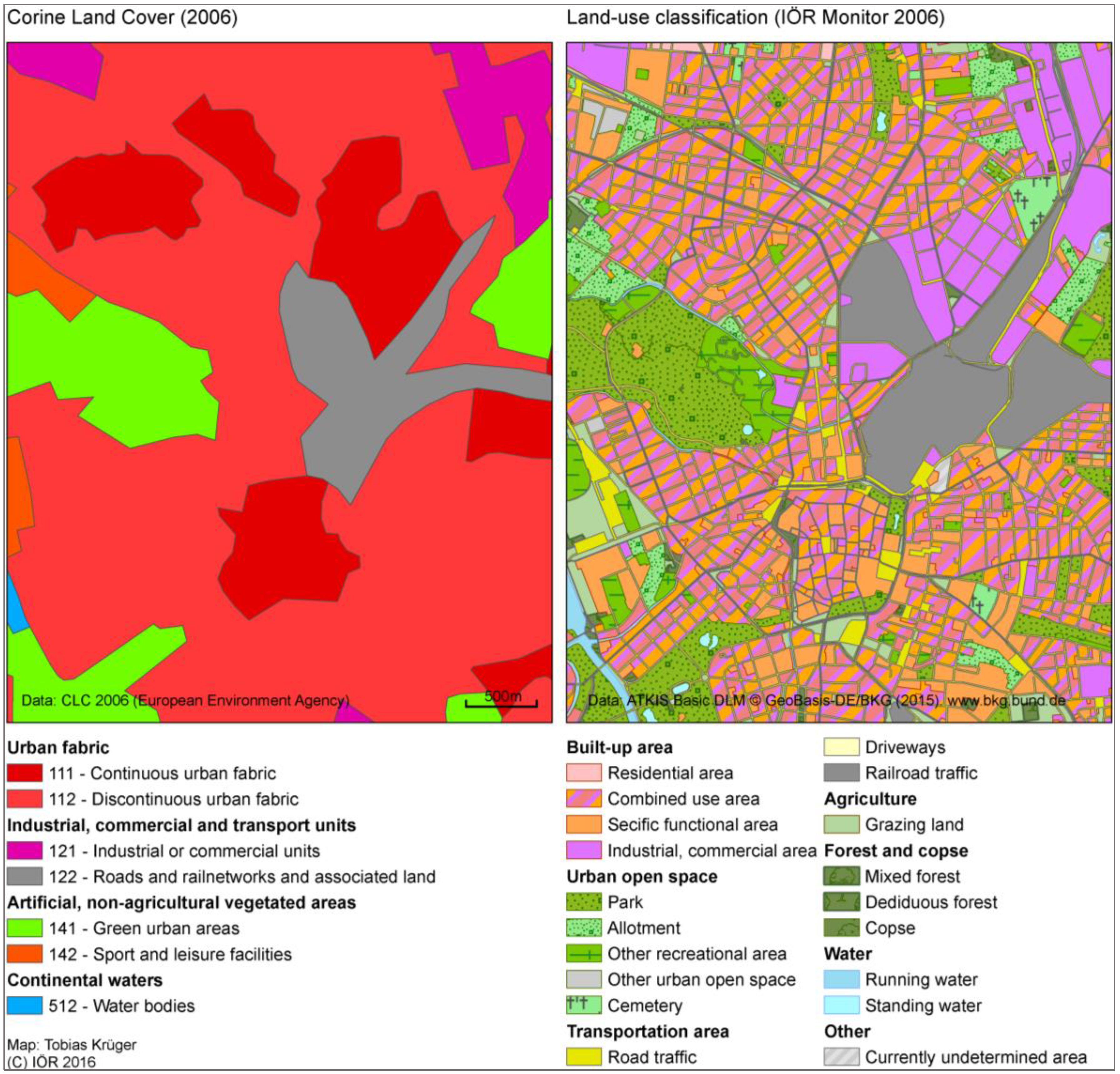
Along with the ATKIS migration, the mapping agencies in Germany have changed the cartographic projection from Bessel/Gauß-Krüger (Zones 3 to 5) coordinates to ETRS1989/UTM (Zones 32, 33) coordinates. This study was done using the ETRS1989/Lambert Azimuthal Equal Area projection (with origin at 52°N, 10°E) as recommended for INSPIRE conformal geographical data [25]. Therefore, the data pre-processing includes a re-projection of the whole Basic DLM dataset of one year. The resulting impact on area sizes has been evaluated as negligible (less than 0.1% of the total area of the country. A visual comparison of the land use classification based on Basic DLM data compared to CORINE Land Cover is shown in Figure 1. As can be seen from the map, the national dataset provides much more geometrical precision and semantic differentiation than the European CLC data. Hence, the ATKIS Basic DLM have been chosen as suitable input data for land use analyses for this study.

2.1.4. Data Pre-Processing

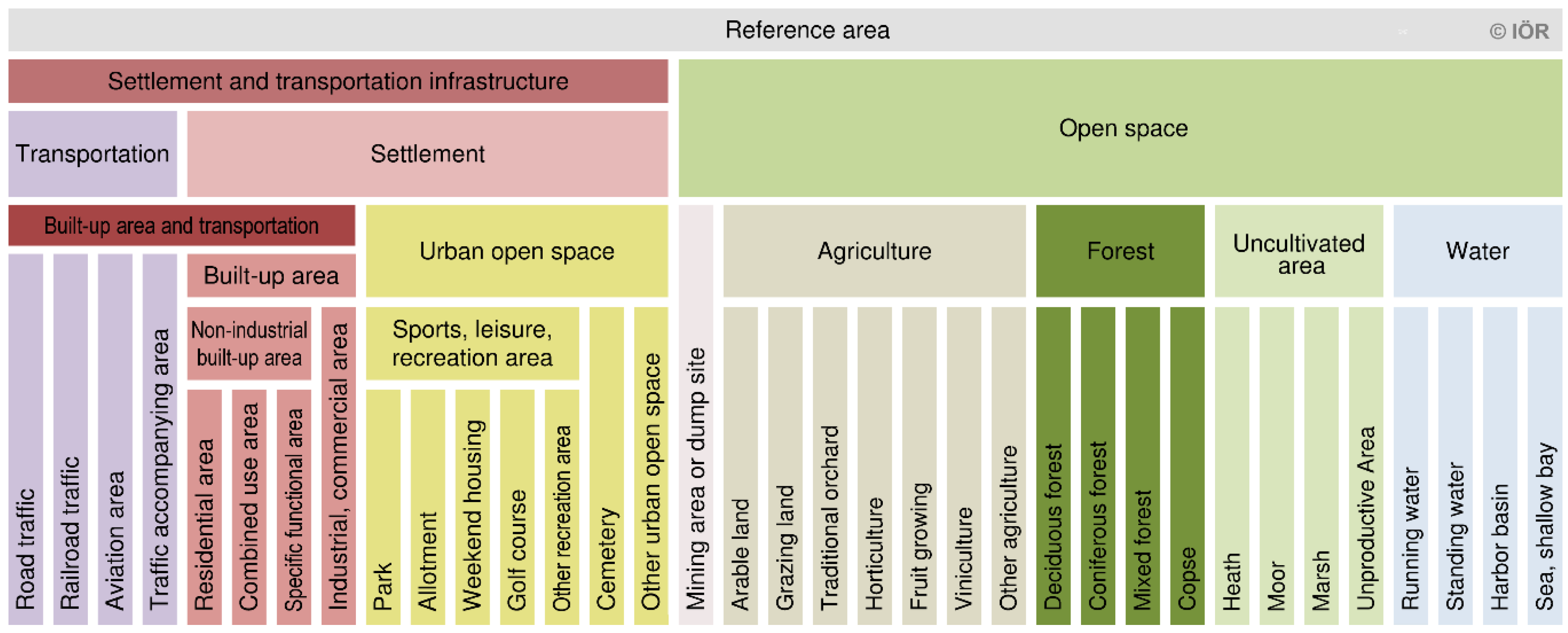
Based on the ATKIS object catalogue [23] and (for the most part) in accordance with the official land use nomenclature used by the Federal Statistical Office [26], a land use typology has been defined (Figure 2). The three main land use classes settlement (including built-up areas and urban open space), transportation (including all areas exclusively used for traffic, except shipping) and open space (including all areas not directly used for settlement or transportation) are hierarchically sub-divided to ensure that each piece of land is part of exactly one land use category, each of them being assigned to ATKIS feature types and attributes. Overlapping land use situations, such as bridges, tunnels or underground objects, are not modelled. In these cases, the top-most land use is defined as dominant.

Since the transportation network consisting of motorways, roads, driveways and railways, as well as running waters, such as narrow brooks, streams and rivers, are modelled as polylines in the input data, these objects are buffered to get polygon representations. The buffer value definition is based on the appropriate width attribute assigned to the polyline object. In cases of invalid or ambiguous object width specification, standard values are used for the buffering. Otherwise, the portion of the Earth’s surface that is covered by transportation infrastructure and water bodies would be heavily underestimated. Buffered features always override the land use information of their neighboring polygons [27,28,29].

A major issue of the Basic DLM is the varying topicality of the data due to the updating cycles, which is realized by updating tiles comparable to a traditional mapping sheet division, of the mapping agencies, which can cause topicality differences of several years. Meta-information provided together with the actual DLM data indicates the date of the latest regular basic updating (German: “Grundaktualisierung”). Furthermore, changes of several important feature types (especially transportation infrastructures) are updated within a short-term cycle of less than one year (German: “Spitzenaktualisierung”). Therefore, ATKIS data have always a certain delay of topicality, which differs throughout the country.

However, it is not possible to generate a dataset of homogeneous data topicality for the whole country. Therefore, the calculation of difference indicators referring to a certain period of time like land take requires the definition of a specific time reference for the whole dataset. Thus, we decided to use datasets of a five-year range regarding their date of delivery to make sure that each federal state has run through at least one updating cycle.

2.2. Determination of Land Use Changes

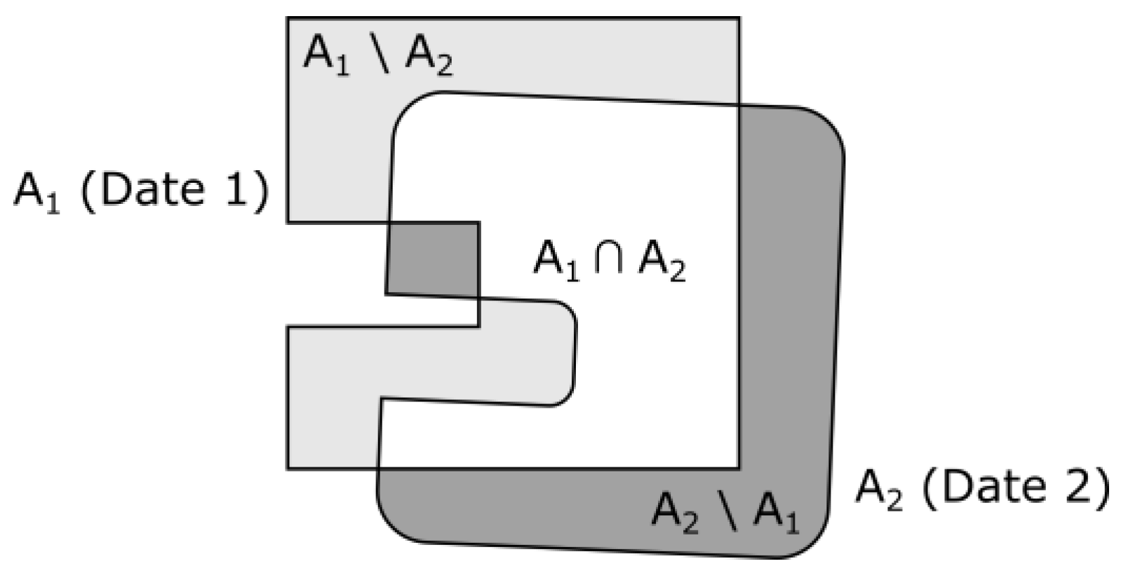
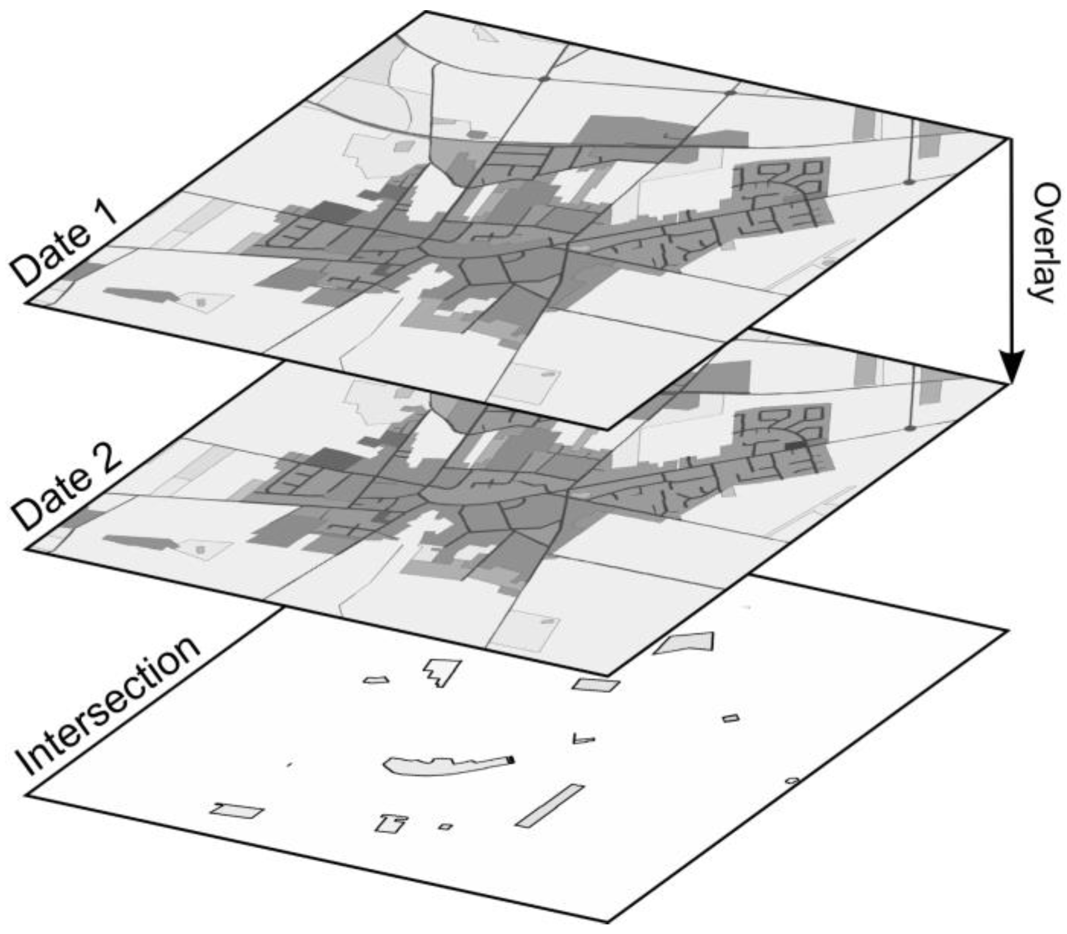
The identification of land use changes between two separately prepared time slices Date 1 and Date 2 is based on the principle of a spatial intersection of the two datasets (Figure 3). The objects of the resulting intersection carry the attributes of both input datasets. Therefore, land use change for distinct areas can be identified for the overlapping areas of the Date 1 and Date 2 data.

Figure 4 shows the overlap of model representations of the same object of land use class A for two different time slots. Due to the geometrical differences of objects, the intersection of the patches causes three different potential result categories: (1) unchanged area, which is the actual overlap of both polygons (A₁ ∩ A₂); (2) non-overlapping areas, which are covered by one of the polygons, which indicate a decrease (A₁\A₂) or (3) an increase (A₂\A₁) of A, respectively.

In general, by applying overlapping procedures, which are widely implemented by standard GIS intersection and symmetrical difference procedures [30], it is evident that parts of the land use class A are converted into another land use class B (≙ A₁ ∩ B₂) or have been converted from B (≙ B₁ ∩ A₂). The difference of disappearing areas of A and those that came to addition equals the net balance NB of the land use change of A:

NB (A) = Area (A₂\A₁) − Area (A₁\A₂) ≡ Area (A₂ ∩ B₁) − Area (A₁ ∩ B₂)

(1)

The number of possible land use change combinations (including the unchanged land use A₁ = A₂) is defined by the square of the number of indicated land use classes. The 35 categories according to the land use typology therefore result in 35² = 1225 combinations. This number can be decreased by aggregating to superior land use classes.

2.3. Geometrical Object Shifting

In many cases, small shifts of vertices and polyline segments can be observed. Thus, the polygon borders of the intersected datasets are not exactly the same, even if the actual real-life objects did not change. Actually, the ATKIS Basic DLM shows these shifts for polygon borders, as well as for linear objects regardless of object types or object attributes. At the very most, the coordinate differences between corresponding polyline vertices are smaller than the acquisition accuracy, which is defined with ±3 m for linear objects and ±15 m for polygon object edges. This has little effect on a mere numerical comparison of land use classes. However, there is an enormous influence on land use change analyses by the spatial intersection method due to resulting sliver polygons pretending land use transformations that did not occur in reality.

Geometrical differences might be caused by human interpreters or by technological procedures. Possible reasons are:

• Increase in the quality of data used for updating (e.g., aerial imagery with higher resolution),
• Changed visibility of object edges due to the phenological vegetation status,
• Employment of different input data sources (e.g., terrestrial surveying data instead of aerial imagery),
• Modified object modelling criteria (e.g., changed minimum patch sizes for mapping),
• Geometrical object generalization (e.g., vertex thinning),
• Coordinate transformations.

In order to get a high quality land use transformation model, it is necessary to detect these coordinate shifts reliably. Therefore, a methodology for the analysis of overlapping land use datasets has been developed allowing for the detection and removal of undesired sliver polygons from the analysis. It is based on the assumption that the movement of land use patch edges within a permitted tolerance does not represent land use changes in reality. The tolerance values for linear and polygonal objects can be set separately as parameters that enable the operator to find the best fitting settings for the data.

2.3.1. Edge Shifting Tolerance of Areal Objects

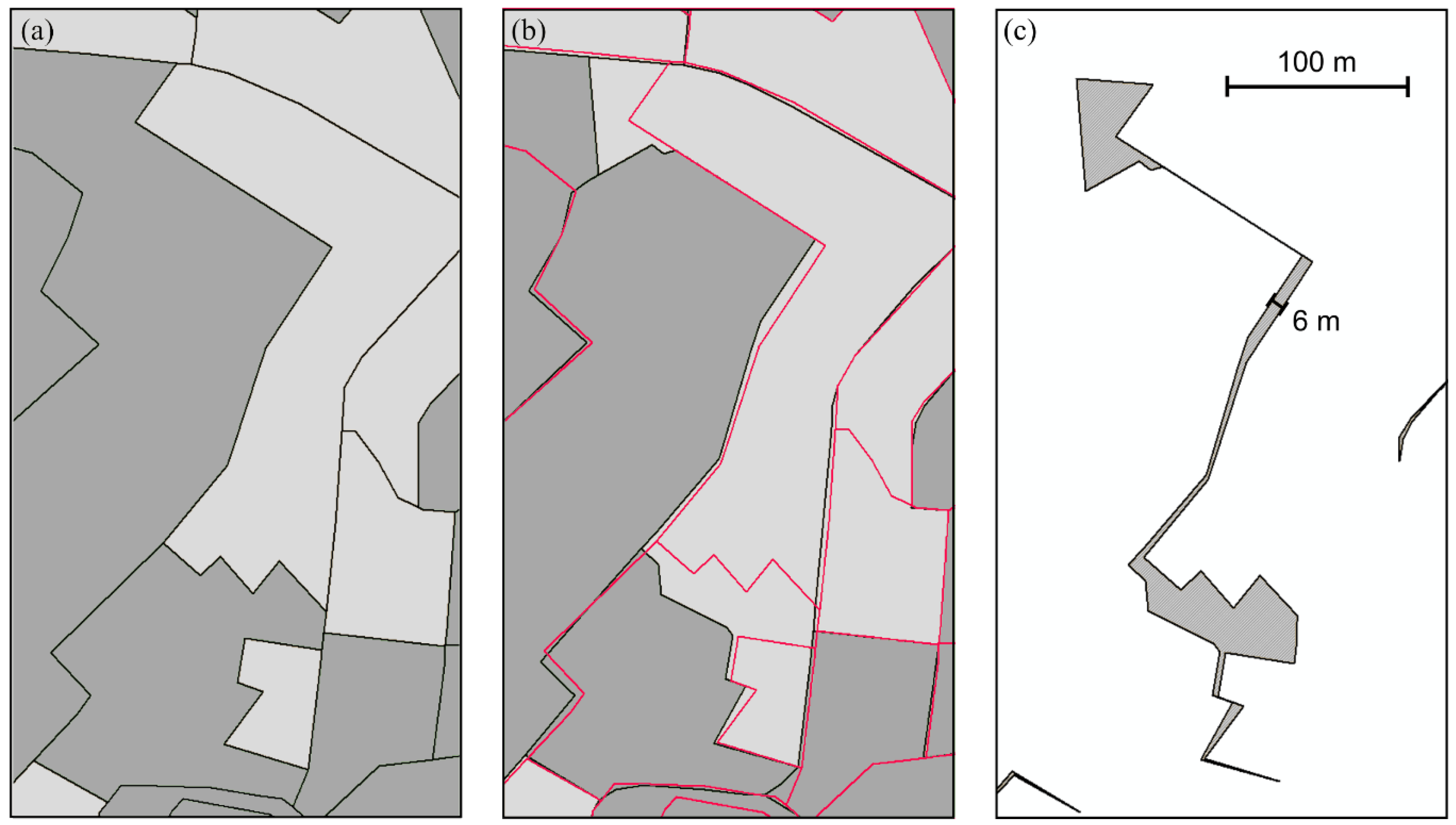
Small shifts of a common edge of adjacent polygon objects cause sliver polygons when intersecting two subsequent datasets. Thus, even if the real-world situation is unchanged, a land use change would be detected. Figure 5 shows the effect of minor corrections of edge vertices on the change detection resulting in undesired sliver polygon patches in addition to real changes, which show up as bigger polygons. Mostly, real changes and sliver polygons occur in combination (Figure 5c).

A simple approach to clean up the intersection is to apply a threshold of minimal resulting polygon areas. All polygons that are smaller than the defined minimum size would not be included in the land use change analysis. Hence, this method would not preserve them from taking into account sliver polygon parts that are connected with real changed objects (Figure 5c) or that exceed the threshold size in the case of very long narrow objects.

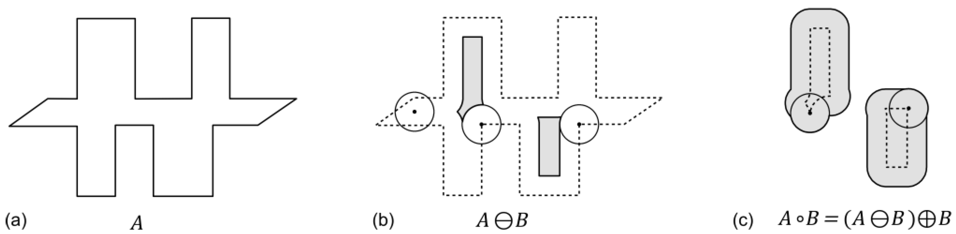
However, it is possible to significantly reduce these objects by methods of morphological filtering [31]. The fundamental operations of morphological filtering are dilation and erosion (Figure 6). In both cases, a structure element B is moved along the polygon borders and relocates its edges. In the case of an outward or inward positioning of B, the objects size increases or decreases, respectively. The operators can be understood as an object buffering with positive or negative buffer distances.

The combined application of these two basic operations are referred to as closing or opening, depending on their succession. Closing applies a dilation before an erosion and is suitable for filling small gaps between or perforations within objects (Figure 7). Opening means to apply the dilation operator right after an erosion in order to eliminate objects appendices (Figure 8).

Closing:

A • B = (A ⊕ B) ⊖ B

(2)

whereby A = original object; B = structure element; • = closing operator; ⊕ = dilation operator; ⊖ = erosion operator.

Opening:

A ◦ B = (A ⊖ B) ⊕ B

(3)

whereby A = original object; B = structure element; ◦ = opening operator; ⊕ = dilation operator; ⊖ = erosion operator.

In order to eliminate the above-mentioned undesired effects of sliver polygons, the opening operator can be applied. Given that the erosion and dilation of the opening and closing procedures are performed with identical structure elements, the resulting objects have nearly the same dimension of their originals. In most cases, the result will have rounded edges depending on the shape of the structure element.

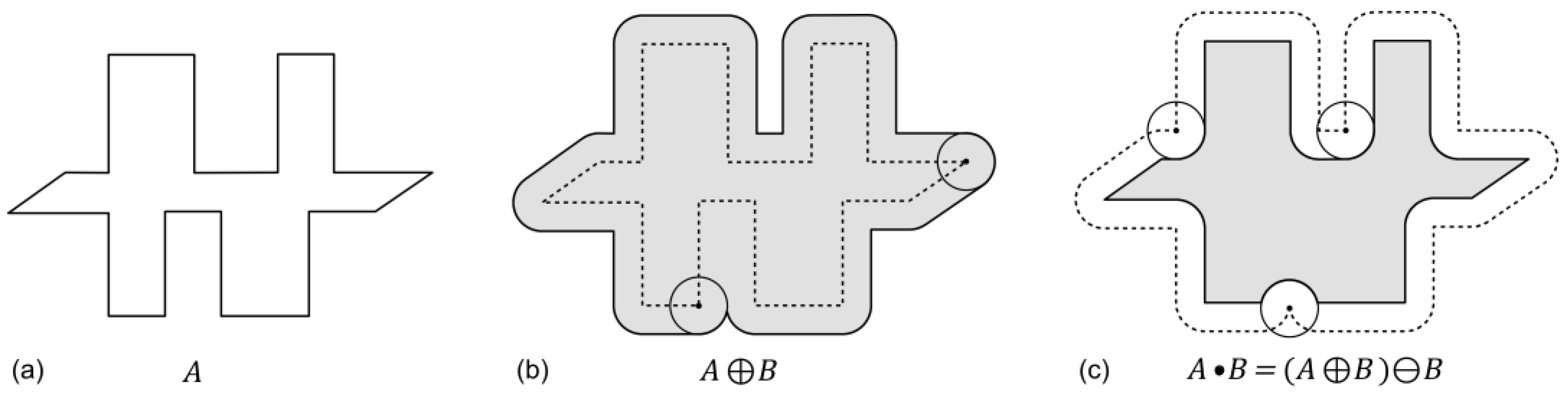
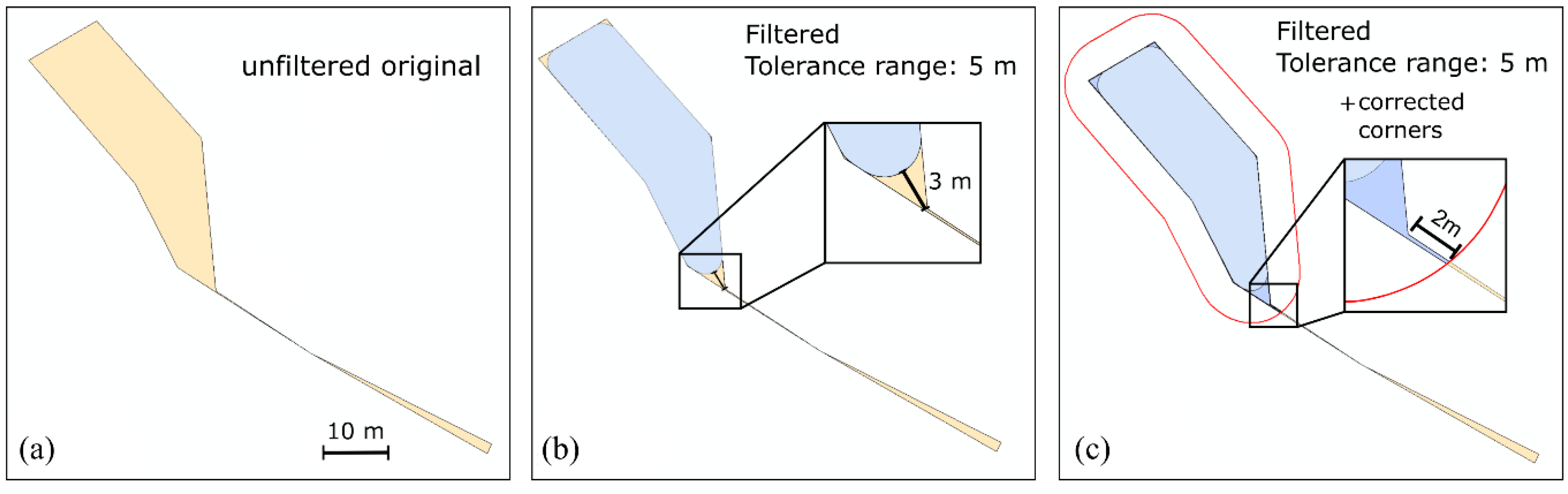
These rounding effects can be minimized by a second correction procedure, which is based on the intersection of the original feature with a once more dilated opening. The principle of the correction is shown in Figure 9. The left and middle subfigures show the unfiltered objects and the opening result. The red line in Figure 9c indicates the dimension of the further dilation, which is used to intersect with the original feature resulting in a feature that is nearly identical to the original shape, except small appendices at polygon corners.

This procedure sequence, which is called corrected opening, can be formally describe as follows: corrected opening:

A_C = ((A ◦ B₁) ⊕ B₂) ∩ A

(4)

whereby A_C = corrected object; A = original object; B₁ = structure element (shifting tolerance); B₂ = structure element (corner correction); ◦ = opening operator; ⊕ = dilation operator; ∩ = intersection.

After the first processing step (i.e., dilated opening) the remaining objects that have not been removed are slightly larger than their originals. The second processing step (i.e., intersection with the original feature) can cause small spikes occurring at the polygon corners (Figure 9c). Since B₁ is defined by the position accuracy (or the allowable edge shifting tolerance, respectively), it has to be kept constant for all objects, regardless of their size. The dimension of the remaining spikes after the intersection with the original features is limited by the size of B₂, which can be adapted in relation to the filtered object size in order to minimize the appendices’ dimensions. However, due to the tiny total effect on the objects’ area, which can be estimated as negligible, B₁ and B₂ can conveniently be defined as identical.

To avoid the erroneous classification of small objects as undesired sliver polygons, an additional corrected opening on the input datasets (not the intersection result) is applicable. Objects that are filtered from the original feature classes can be flagged and later excluded from the final corrected opening after intersection. Thus, those small objects are not removed, and land use changes of minor size will remain in the data.

2.3.2. Line Shifting Tolerance Filter for Linear Objects

In the case of linear objects, the objective is to distinguish the ones that have been added or removed in the second dataset from those that have just been adjusted by shifting vertices in the updating process. As shown by Krüger et al. [28], linear objects of transportation and hydrological networks have to be buffered in order to get a polygon representation of these features. Since most of the buffered objects are still narrow with respect to the structure elements that are applicable to polygon objects, the corrected opening procedure would end up in a broad elimination of features. That is why the morphological filtering cannot be applied to those polyline-buffered objects.

The correspondence of line features in different datasets can be analyzed by the “simple positional accuracy measure for linear features” [32]. Corresponding polylines are mutually defined as references that have to be buffered to a certain distance, which is defined by the valid maximum position shift between the pairs of lines. The compared dataset is then evaluated against this buffer zone, whereas polylines within the tolerated range of their corresponding counterparts are evaluated as correct. Features outside the buffered tolerance zones either have no corresponding polyline or have incorrect geometrical positions (Figure 10).

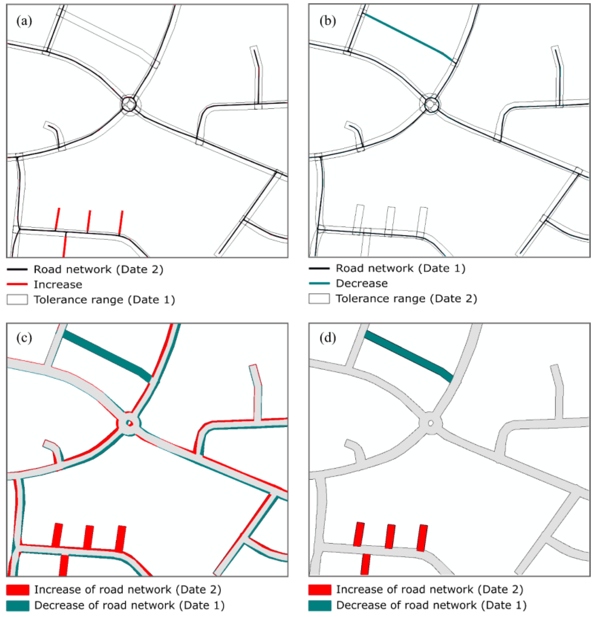
Transferred to the issue of comparing land use datasets, this method can be adapted to check for the development of feature networks, such as streets or railway lines. Applying the buffer-based positional accuracy measurement allows for the differentiation of actually changed (or new) objects from those that just have been corrected. To get an evaluable set of new or disappeared objects, either of the compared datasets has to be evaluated against the buffer zones of the other one.

The buffer distance for the evaluation of the positional accuracy measurement should be defined in correspondence to the accuracy parameters of the input data. In case of the ATKIS Basic DLM, this value is set to 3 m [33].

Figure 11 shows an example of the comparison of two road network datasets of different years. In the upper left subfigure, the more recent network has been evaluated against the buffered previous data resulting in the detection of new streets. The upper right subfigure shows the opposite procedure of checking the older network against the buffered more recent data, which enables one to detect features that haven been removed.

2.4. Semantical Object Shifting

Besides the effects of geometrical differences, object types and object attributes can be altered even if there is no change in the real world. This can be caused by modifications of the data model, or by introducing new attributes, or merely by editing object attributes (e.g., information on road width). The effects of model-based data modifications can bias the result of a bi-temporal land use change analysis significantly. Therefore, it is desirable to get information about changes that are caused mainly by recording rules, rather than by real-world changes.

With respect to the ATKIS Basic DLM, which was used as input data for this study, several issues arise. Since the dataset had its early beginnings before 1990, it has been migrated to a new model scheme demanding a complete re-design of the Basic DLM definitions [34]. The migration process was not realized simultaneously in all federal states, but lasted from 2009–2013 [35]. Thus, 2008 was the last year before the first federal states migrated to the new data model, and 2013 was the year of its earliest nation-wide availability.

As shown in a previous study, several specific effects of the data migration could be revealed, which are mainly caused by the introduction of new objects classes or by altered modelling approaches of topographic features [36]. Changed model definitions of two of the major object classes have impacts on the geometrical shape and the attribution of the polygons of allotments and polygonal road traffic features; neither of them were defined in the older Basic DLM version. The introduction of these object definitions caused re-assignments of the affected features, resulting in object class transformations without real land use changes. Another major aspect is currently undeterminable areas, which have been significantly reduced in number and covered area. This category is used for uncertain land usage or inappropriate object modelling definitions in the object catalogue. Since this object type will be entirely removed in the upcoming reference Version 7.0 of the ATKIS object catalogue [37], it is highly unlikely that intersections of those polygons with other land use classes indicate real land use changes.

3. Implementation and Testing

In the following, the results of the present approach to the tolerance-based intersection of land use geometry is described. The methodology was implemented in an ArcGIS and FME software environment for the geo-processing parts and was automated with Python. The analysis of the intersection results by means of selective filters and aggregation rules for superior land use classes was then realized by SQL database queries.

3.1. Input Datasets

The proposed methods were tested on land use datasets derived from ATKIS Basic DLM data, which had been pre-processed according to [28,38]. The comparison of the land use data for the years 2008 and 2013 shows slight changes in the proportions of the main land use classes. It is obvious that the land use categories with the largest growth benefit from the loss of agricultural land (

Table 1. Main land use classes in Germany (absolute area and percentage change, reference years 2008 and 2013).

Land-Use Class	2008		2013		Difference
	Area (km2)	Share (%)	Area (km2)	Share (%)	Area (km2)
Urbanized Area	40,313.6	11.3	42,272.3	11.8	1958.7
Built-up area	27,179.2	7.6	28,040.6	7.8	861.4
Urban open space	3623.0	1.0	4147.8	1.2	524.8
Transportation	9511.4	2.7	10,083.9	2.8	572.5
Open Space	317,398.3	88.7	315,402.4	88.2	−1995.9
Agriculture	193,362.7	54.1	188,467.9	52.7	−4894.8
Forest	112,445.2	31.4	113,035.5	31.6	590.3
Water	6786.9	1.9	6852.4	1.9	65.5
Other	4803.5	1.3	7046.6	2.0	2243.1

). However, as mentioned before, the mere juxtaposition of the absolute or relative values does not clearly indicate the actual transformation processes between the several land use classes. In addition, summed-up national statistics cannot reflect regional or local differences in the dynamics of land use change.

3.2. Intersection Results

3.2.1. Unfiltered Intersection

Table 2. Geometrical parameters of the intersection result of the input datasets.

	Dataset 2008	Dataset 2013	Intersection
Number of Polygons	9,477,378	9,554,043	38,164,746
Area of Polygons (m2)
Mean	37,743.8	37,436.9	9373.5
Standard deviation	175,053.7	177,832.2	82,771.2
Median	5138.0	5274.9	7.6
Unchanged area sum (%)			93.1
Changed area sum (%)			6.9
Number of change combinations			1225

indicates geometrical parameters of the input datasets and the resulting intersection of both. As one can see from these numbers, the mere intersection is not quite appropriate for a deeper analysis of land use transformation, since according to the median value of the intersection, the majority of the resulting polygons are of a very small size and therefore are unlikely to represent real-world situations. In fact, the MMU for many topographic features in the ATKIS Basic DLM is 1000 m² unless the topological networks of transportation lines and running waters build up smaller meshes to be filled. Hence, the resulting polygons of the intersection should not turn out to be considerably smaller than this value.

In

Table 3. Cumulated effects of small intersection polygons with changed land use classes for Germany.

Feature Size (m2)	Changed Polygon Number		Changed Polygon Area
	Absolute	% of Total	Absolute (km2)	% of Total
<10	18,699,964	65.9	18.5	0.1
<100	22,937,834	80.8	183.6	0.7
<1000	26,388,785	93.0	1392.4	5.6
<10,000	27,894,965	98.3	6469.4	26.2
all	28,385,019	100.0	24,683.7	100.0

, the cumulated effect of the resulting small-sized polygons is tabulated. Ninety three percent of all changed polygons are smaller than 1000 m² and represent not more than 5.6% of the total changed area, which turns out to be 0.4% of the area of Germany. Usually, the reduction of changed polygons for the change detection is effected by the definition of a threshold. However, this would not entirely remove misclassified features, because sliver polygons can cover relatively large areas, especially along roads if the road axes have been shifted or the width attributes have been modified. Therefore, a reliable land use change analysis requires the filtering of undesired effects as proposed in this paper.

3.2.2. Position-Corrected Intersection

The application of the tolerance filter regarding the edge shifting has immediate effects on the balance of detected land use changes. Since filtered regions along the edges of slightly modified object geometries do not count for the land use change modelling, the absolute number, as well as the resulting areas of the polygons that have to be considered for land use transformation analysis decrease compared to the unfiltered intersection. Generally, the absolute number of the filtered objects depends on the frequency of positional corrections applied in the updating cycle of the original Basic DLM. Thus, the more often vertices have been shifted, the greater is the difference of the unfiltered computation of changing areas from the filtered result. It is to be observed that the intensity of position corrections is not evenly distributed over Germany, but varies within the federal states. Therefore, in order to achieve comparable results for different federal states, it is recommendable to apply the position correction. Otherwise the resulting data will probably show regional differences.

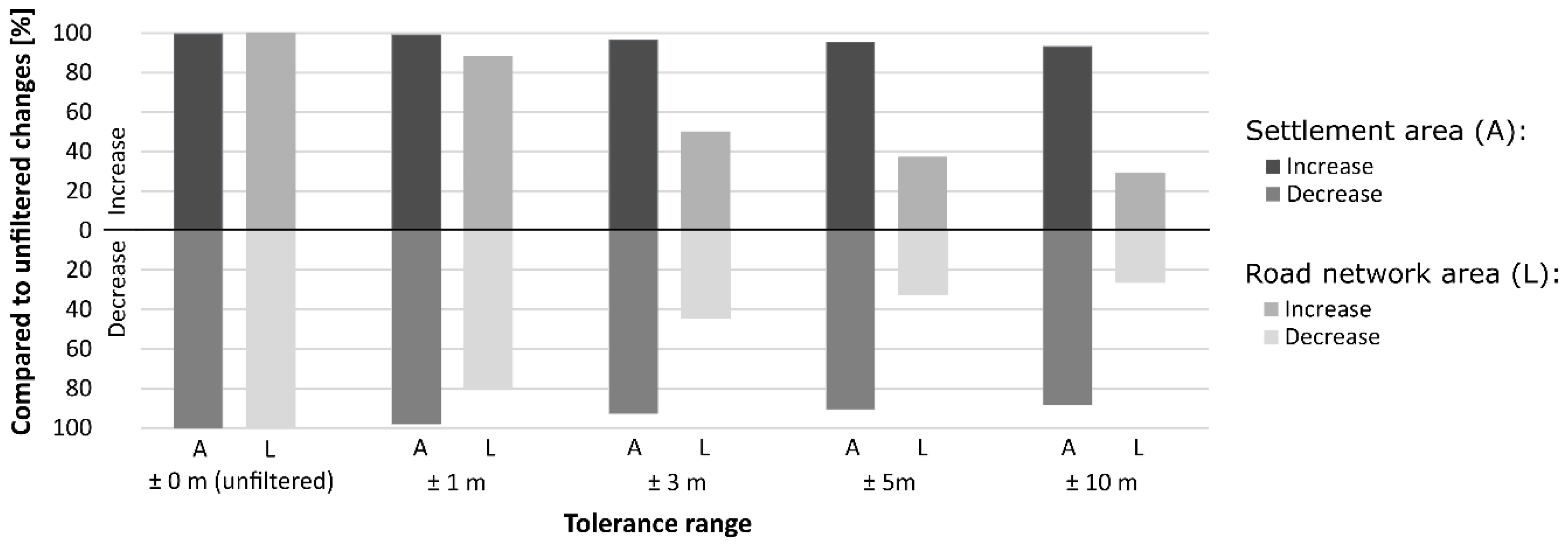
Figure 12 shows the effect of applying the filter to eliminate shifting edges for different tolerance values, which are considered as valid maximum deviations of the object vertices. This analysis has been carried out for the federal state of Schleswig-Holstein. Schleswig-Holstein was identified as one of the federal states showing numerous position shifts of polylines and polygon edges. Therefore, the measured effects of the application of different values of the filter tolerance are clearly perceptible.

In the diagram, the area covered by the road network has been analyzed separately from the summation of all other land use classes that are subsumed in the settlement category. The diagram bars indicate the ratio of area change that can be observed for the two land use categories when applying tolerance values regarding shifting edges in comparison to the uncorrected intersection result.

It is obvious that the filtering leads to a reduced detection of transformed settlement and transportation areas. The area of the category road traffic reacts very sensitively to a stepwise increase of the line shifting tolerance. Here, a tolerance value of 3 m leads to a cut-off of more than 50% of the detected transformed road traffic areas of the land use change analysis. Settlement, on the contrary, largely consists of polygon features (e.g., built-up areas, airports, urban open space), which are relatively robust against increasing values of the edge shifting tolerance.

According to the data providers, the position accuracy of the ATKIS Basic DLM is ±3 m for an essential linear object, such as roads, railways or running waters. The general positional accuracy for polygon objects is given as ±15 m [39]. Therefore, a separate processing of linear (buffered) and areal objects is necessary to achieve reliable results.

3.2.3. Semantical Shifts Reduction

As described in Section 2.4, the intersection of two datasets is biased by systematic model changes. The results of this analysis show that several specific transitions between land use classes should be dropped from the land use change detection, because there have been some re-classifications made of object types that do not represent real changes, but that realize data corrections [36].

The largest influences on the results of the land use change analysis could be found for the following land use class transitions:

• Commercial area vs. mining area:

In the older ATKIS object definitions, the overlapping of so-called basic area objects (German: “Grundflächenarten”) was allowed for certain situations, although these objects were determined for a non-redundant coverage of the Earth’s surface. In fact, nearly all possible overlapping combination can be found in the data. There are also many extensive opencast mining sites that are indicated both as mining sites and as industrial or commercial areas. The new ATKIS modelling rules strictly forbid overlapping features for objects of the actual land use category, to which both industrial/commercial and mining areas belong. Thus, after the migration of the data, major transitions between these two categories are to be expected.

This indeed affects the balancing of land take analyses, since in the land use typology, industrial and commercial area is part of urbanized areas, whereas mining areas (within mining area or dump site category) belong to the open space. Hence, the intersection result of datasets that incorporate both the previous and current versions of ATKIS data should be cleaned from transitions between these two land use classes, because these in most cases do not represent real-world changes.

• Horticulture vs. allotment area:

Because allotments were not defined as an object type in the object catalogue of the older Basic DLM, most of the corresponding area was modelled as horticulture. This is a problem since allotments contribute to urban open space (and therefore, to the urbanized area), whereas horticulture is an agricultural land use category belonging to the open space. In order to get an estimated differentiation between these two classes, allotment areas were separated from horticulture by intersecting the latter with the object class locality, indicating a generalized settlement area (German: “Ortslage”). As a result, the horticultural area within the communal settlement area was designated as allotments. However, the definition of the object class allotment (German: “Kleingarten”) has been introduced in the new ATKIS Basic DLM, which made it necessary to transfer the horticulture polygons into a proper land use class. The general approach to migrate these areas into the new dataset consisted of two steps: firstly, all corresponding polygons were classified as one of the two object types in question and, secondly, to assign the correct object type during subsequent updating cycles (so-called “post-migration process”). Therefore, these categories should be excluded from multi-temporal land use analyses until the post-migration process is finished.

• Grazing land vs. traffic accompanying areas:

This land use category was introduced with the new ATKIS object catalogue. It is modelled by polygons of the object type road traffic (German: “Straßenverkehr”). Since no corresponding object type existed in the older model definitions, these areas were often modelled as grazing land due to the vegetation cover. In order to avoid incorrect land use change categorizations, which would indicate a loss of open space to the benefit of transportation infrastructure, the transition of grazing land into road traffic should be excluded from the analysis of land use change.

• Currently undeterminable areas vs. other areas:

By comparing the current reference version GeoInfoDok 6.0 [39] of the ATKIS object catalogue with the draft of the upcoming GeoInfoDok 7.0.1 [37], which will supersede today’s document in the near future, the present object type currently undeterminable area (German: “Fläche zur Zeit unbestimmbar”) will be removed [23,37]. Actually, the summed up areas of that object class show a continuous decrease in the annual ATKIS datasets, which might indicate an anticipation of the necessity to transfer these polygons into proper object types in the future. Therefore, it can be assumed that in the past, this object class had widely been utilized as a placeholder for objects of unclear affiliation. Hence, it is recommendable to exclude these areas from the land use change detection.

Figure 13 shows the absolute effects of the consideration of these land use categories on the quantification of urbanized area transformation between the analyzed 2008 and 2013 datasets. The increase or decrease of urbanized areas is shown by upwards or respectively downwards pointing bars. Expectedly, the absolute increase exceeds the decrease, resulting in the positive net balance of land taking processes indicated by the point signatures. Actually, the largest absolute influence on the net balance actually has the conversion between horticulture and allotment area, which covers about 20% of all detected changes between urbanized area and open space.

3.3. Balanced Filtered Land Use Transformation Analysis

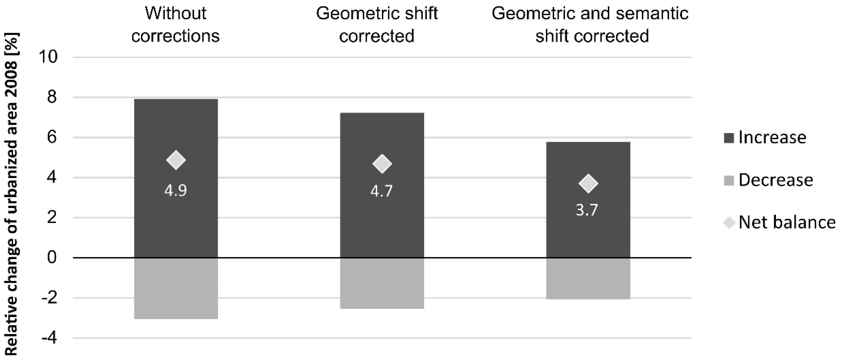
The developed tools for the filtering of edge and line shifting tolerances, as well as of semantical shifts have been applied to the land use datasets of 2008 and 2013. Regarding the geometrical correction, we assumed maximum position deviations of ±3 m and ±5 m for polyline and polygon features, respectively. Therefore, the parameters for the corrected opening were set to a 6-m line shifting tolerance and a 10-m edge shifting tolerance.

Figure 14 shows the effect of the filtering on the detected land transformations between urbanized areas and open space. The left bar indicates the results of the uncorrected intersection, which sums up to a net increase of urbanized areas of 4.9% from 2008–2013. The correction for geometrical shifts has a minor effect of reducing the net balance to 4.7%, whereas the additional correction for semantic shifts (adjusting for known effects of the ATKIS model migration) brings the value down to 3.7%

Table 4. Relative changing rates (%) of the transformation between urbanized area and open space from 2008–2013 for Germany, differentiated into subcategories.

		Urbanized Area *
		Built-Up	Transportation	Urban Open Space	Total
Open Space *	Agriculture	+2.9	+0.7	+0.6	+4.2
		−0.6	−0.3	−0.2	−1.1
	Forest/Copse	+0.3	+0.9	+0.2	+1.4
		−0.2	−0.2	−0.2	−0.6
	Other	+0.1	+0.0	+0.0	+0.1
		−0.2	−0.0	−0.0	−0.3
	Total	+3.3	+1.7	+0.8	Total Net Balance +3.7
		−1.0	−0.6	−0.5

* Positive sign (+), change from open space to urbanized area; negative sign (−), change from urbanized area to open space.

shows the relative changing rates of the geometric and semantic shift-corrected transformation between urbanized area and open space. The increase of urban area consists mainly of former agricultural land, which comprises arable, grazing and horticultural land, followed by former forest or copse area.

4. Discussion

Land use change analyses based on statistical reports actually reveal the change of the land use structure, i.e., there is per se no information on the conversion of land from one utilization to another. This pure net balance is not suitable to describe or quantify the real dynamics of land use change, since it leads to a “serious underestimation of land change” (cited from [40]). The differentiation between “net and gross land changes” can also be used for the quantification of carbon fluxes altering the atmospheric conditions [41].

In this paper, we presented a methodology for a separate calculation of land use conversions between any recorded land use categories of two (or more) subsequent time slices. Therefore, it is possible to account for both gross and net balancing land use changes.

However, the pure intersection of multi-temporal land use datasets is often not suitable for a localized and high-resolution detection of changes due to sliver polygons that occur in the case of polygon edges or polylines that have a similar, but not identical geometry. Therefore, an adaptive method of intersection is needed that takes tolerable position shifts of land use patches into account. The approach of the balance calculation of land use changes, which is herewith proposed, is based on geo-processing methods that allow for the revealing of the actual transformation of land use. As input data, geo-topographical datasets of the mapping agencies of the German federal states had been prepared and pre-processed. The developed methodology combines approaches of morphological filtering, geo-processing methods and positional accuracy measurements to eliminate undesired effects of a mere intersection of features resulting from minor geometrical corrections due to the updating of the Basic DLM. The parameters can be adapted to the specific conditions of the input datasets, i.e., it is possible to define specific tolerance ranges for polygon and line features depending on the accuracy specification of the input data.

Furthermore, alterations of the object type or modifications of the object attribute can be excluded from the land use change balancing in order to eliminate wrongly-detected land use transformations. This effect has previously been described and referred to as “methodological change” in the data [42]. These include the repeatedly observed re-classification of arable land and grazing land, for instance. The methodology is based on the application of tolerance filters that take the geometry of objects into account, which can happen to be slightly modified during the up-dating process, even if there is no change in reality.

Thus, land take can be described not only numerically by the proportions of land use categories, but rather by the transformation of the actual land use. In this way, land transformation processes can be identified and localized for the whole country. Thus, it is possible to detect the main sources that contribute to the ongoing increase of settlement and transportation infrastructure. Generally, this knowledge can help to understand land transformation processes and to identify drivers of land use change.

Therefore, the proposed methodology is suitable for a reliable comparison analysis of two land use classification datasets. The implementation and testing of the approach has been performed in the context of the Monitor of Settlement and Open Space Development, which provides annual indicators for land use structure in Germany with high spatial resolution [29]. The derived land use datasets for two years covering the whole country including 35 differentiated land use classes have been analyzed.

However, the implementation and testing of the approach revealed several issues that need to be solved in the future.

In the case of buffered features (e.g., transportation, hydrology), it is possible to process the centerlines separately as described in Section 2.3.2. Otherwise, it might be necessary to create centerlines, to decrease the size of the structuring morphological element or to exclude these narrow input objects from geometric filtering by using corrected opening (before the intersection).

The second major problem is the detection of altered model definitions or data corrections in the input datasets. Here, expert knowledge is necessary to distinguish real changes from model modifications or data corrections. Therefore, the introduction of object attributes indicating meta-information on the reasons for object manipulations should be considered by the data providers. Of course, in any case, it is necessary to check the analysis results for plausibility and consistency.

Further, it is recommendable that the compared datasets have undergone a complete up-dating period. Otherwise, data that have not been reviewed and therefore actually represent the same state of land use would be included in the comparison. For the federal states in Germany to ensure a five-year update cycle for the entire Basic DLM dataset, the land use change analysis should also span at least a five-year period.

5. Conclusions

As shown in this study, multi-temporal datasets of high resolution landscape models (in this case, the Basic DLM provided by the mapping agencies in Germany) cause some problems when used as input for analyses regarding land use change. Due to geometrical shifts of polygon edges or linear features, such as roads, driveways, railways and running waters, a mere intersection of two (or more) datasets results in numerous undesired sliver polygons that indicate pseudo-changes of land use that do not represent real-world conditions. Further, modifications of the data model or changed mapping rules can falsify the results of change detection.

Especially for small-scale studies with the focus on locally-determinable changes, these effects can considerably affect the reliability of the results. The presented methodology of tolerance filters regarding edge shifting and line shifting as part of the intersection process allows for the detection and elimination of small geometrical modification effects.

Furthermore, the presented methodology can be used for data evaluation. By the localized determination of previous and subsequent land usages, it is possible to look for unique transformation rates that exceed the usual dimensions of land use change in comparable regions. In this case, it is an indicator for modifications in the data model, object modelling rules or mapping habits. Accordingly, different strategies for the boundary delineation of built-up areas can be observed throughout the federal states. For efforts to harmonize data between federal states, the related data modifications can lead to changes concerning both geometrical shape and attributes of the objects despite no actual change. For small-scale study areas, these effects have more relative impact than for large-scale study areas due to the proportion of the patch sizes of the involved polygons with respect to the study area.

As a conclusion, it can be stated that the proposed methodology is feasible for DLM datasets regarding the analysis of land use change. The filtering methods allow for the elimination of undesired effects that occur due to small differences in the object edges and vertex positions of linear features, which ensures a high reliability of the results.

This way, it is possible to identify and localize actual land transformation with higher precision than just comparing the statistical values of proportions of land use classes of different years. This can contribute to the understanding of land taking processes, which is essential for sustainable spatial development policies.