A MongoDB-Based Management of Planar Spatial Data with a Flattened R-Tree

Abstract

This paper addresses how to manage planar spatial data using MongoDB, a popular NoSQL database characterized as a document-oriented, rich query language and high availability. The core idea is to flatten a hierarchical R-tree structure into a tabular MongoDB collection, during which R-tree nodes are represented as collection documents and R-tree pointers are expressed as document identifiers. By following this strategy, a storage schema to support R-tree-based create, read, update, and delete (CRUD) operations is designed and a module to manage planar spatial data by consuming and maintaining flattened R-tree structure is developed. The R-tree module is then seamlessly integrated into MongoDB, so that users could manipulate planar spatial data with existing command interfaces oriented to geodetic spatial data. The experimental evaluation, using real-world datasets with diverse coverage, types, and sizes, shows that planar spatial data can be effectively managed by MongoDB with our flattened R-tree and, therefore, the application extent of MongoDB will be greatly enlarged. Our work resulted in a MongoDB branch with R-tree support, which has been released on GitHub for open access.

1. Introduction

Sensing and information technologies have brought us into the era of so called “Big Data” [1,2]. Traditional relational databases, limited to normalization demand [3] and atomicity, consistency, isolation, and durability (ACID) guarantee [4], perform poorly in coping with the pressing demands of “Big Data” applications, such as massive data storage, high concurrency access, convenient horizontal scalability, etc. Recently, more and more NoSQL (Not Only SQL) databases [5,6] are developed to challenge “Big Data”, like BigTable [7], Dynamo [8], Cassandra [9] and MongoDB [10]. Among them, MongoDB is a document-oriented open-source database with dynamic schema, rich query language, and high availability, attracting more and more industries to experience its power. For example, Adobe uses MongoDB to store petabytes of data in the large-scale content repositories underpinning the Experience Manager; eBay uses MongoDB in the search suggestion and the internal Cloud Manager State Hub. In addition, MongoDB starts to play an important role for researchers to store their scientific data. For example, Jiang et al. developed a MongoDB-based clustering storage system for unstructured data [11]; Long et al. used MongoDB to manage building modeling components and their metadata [12].

Among “Big Data”, a large proportion is explicitly or implicitly linked with spatial locations, such as earth observation data, moving object data, commuting OD data, etc. In order to manipulate location data, MongoDB adopts the GeoJSON standard [13] to encode geographical data structures and, moreover, it provides 2dsphere index to accelerate spatial query processing. On one hand, various geographical features, including points, line strings, polygons, and their combination, are available in MongoDB. On the other hand, diverse queries, such as point locating, range, and near searching, are supported by MongoDB. As a result, a growing body of studies are focusing on MongoDB to develop spatial applications. Foursquare, a popular location-based service (LBS) provider, has migrated its data to MongoDB to take advantage of its built-in auto-sharding and 2dsphere index; Zhang etc. used MongoDB to carry out parsing, storage, and query of the huge GIS spatial data of the shape format [14]; Lutz et al. addressed the use of MongoDB for the provision of measured and processed massive data collected by the remote sensing instrument GLORIA [15]; Boehm et al. tried MongoDB to store large LiDAR files and allowed spatial queries on the bounding box of the LiDAR tiles [16].

MongoDB’s 2dsphere index actually combines the strength of discrete global grids [17] and B⁺-tree structures [18], which first partitions the Earth surface into cells at multiple resolution levels and then applies a B⁺-tree to index geographical features approximated as one or multiple cells. It means that the 2dsphere index is limited to accept spatial data of geodetic coordinate system (i.e., latitude and longitude) and calculate geometries on the Earth’s surface (note that 2dindex, supporting only point data of a Cartesian coordinate system, was no longer advocated by MongoDB). However, there exists a large number of applications, particularly at the city/country scale, that are still used to apply planar Cartesian coordinates to measure spatial data because of convenient acquisition and straightforward calculation. Planar spatial data collected by these applications, such as land-use data, road network data, and administrative division data, are usually stored in object relational databases, like Oracle and PostgreSQL. One may argue that it is possible to transform planar spatial data under a geodetic coordinate system and then import it into MongoDB. However, such a transformation is neither necessary, nor proper, for spatial data of small scales, because position locating and geometry calculating under a Cartesian coordinate system is more precise, and moreover, Cartesian computation is simpler and more efficient than spherical computation.

It is well known that R-tree [19] is a widely used two-dimensional index structure for managing planar spatial data, and it has already become an essential and indispensable configuration in modern spatial databases. In addition, R-tree attracts a large amount of research work in related academic fields, resulting in quite a few variants of R-tree. To the best of our knowledge, there exists little work in the NoSQL world that addresses spatial data processing powered by R-tree. Actually, most NoSQL products pay much attention on issues like scalability and availability, with little consideration on providing spatial data types, let alone supporting spatial query processing, leaving spatial storage, and processing a fairly difficult task of application development. Though MongoDB applies the GeoJSON standard to embrace spatial data and, therefore, enable spatial functions, it is much more suited to LBS applications owing to its inner indexing mechanism, which means it only accepts geodetic spatial data, failing to deal with planar spatial data.

In order to take advantage of both MongoDB and R-tree, this paper investigates how to effectively integrate R-tree indexes into MongoDB and, therefore, be capable of managing planar spatial data. The core idea is to flatten he hierarchical R-tree structure into the tabular MongoDB collection, in which R-tree nodes are represented as collection documents and R-tree pointers between nodes are expressed as document identifiers for foreign referencing. Firstly, a data schema about the planar spatial data and a flattened R-trees is designed; after that, a module that manages planar spatial data by consuming and maintaining the flattened R-tree is developed, which is then seamlessly plugged into MongoDB’s routing nodes. With this design, not only planar spatial data, but also flattened R-trees, could be distributed among MongoDB’s storage nodes and, moreover, planar spatial data could be loaded and queried with existing interfaces oriented to geodetic spatial data. The experimental evaluation, using real-world datasets with diverse coverage, types, and sizes, shows that planar spatial data can be effectively managed by MongoDB with our flattened R-tree and, therefore, the application extent of MongoDB will be greatly enlarged. Our implementation based on MongoDB 3.2.0 is released on https://github.com/lmars-gis/mongo/tree/v3.2.0/rtree for open access, aiming at benefitting more people in the GIS field.

The remaining of this paper is structured as follows. Section 2 introduces some necessary background knowledge, and Section 3 presents a novel idea to flatten the R-tree structure into a MongoDB collection. In Section 4, the framework to integrate an R-tree module into MongoDB is described and some key integration issues are discussed. In Section 5, spatial data management with a flattened R-tree, including create, read, update, and delete (CRUD) operations, is addressed. Section 6 reports the experimental evaluation by comparing the flattened R-tree and built-in 2dsphere, and finally Section 7 reports our conclusions.

2. Background

2.1. NoSQL and MongoDB

Triggered by the demands of Web 2.0 companies, such as Facebook and Amazon, NoSQL has emerged to provide a mechanism for storage and retrieval of data that is modeled in means other than the tabular relations used in relational databases. A NoSQL database has a distributed, fault-tolerant architecture that does not use SQL as its query language and may not give full ACID guarantees. According to the way they store data, NoSQL databases can be classified into four categories: Key-value databases like Dynamo, Column-Oriented database like BigTable, Document-oriented databases like MongoDB, and Graph databases like Neo4j [20].

Different NoSQL databases provide different advantages for diverse applications. MongoDB, compared with other NoSQL databases, provides more complex query functions against a document-oriented data model. It is a typical distributed clustering system composed of three key components, namely, shard server, config server, and route server. Applications address MongoDB through any one node of the router server, which then dispatches operations to appropriate nodes of the shard server. Data is distributed across all nodes of the shard server, while metadata about distribution is stored in the config server of, at most, three nodes. MongoDB is able to provide auto-distributing capability, which means automatic I/O load balance among multiple shard server nodes, thus guarantees flexible horizontal extension against rapid growth of data.

A MongoDB database is made up of collections, a logic unit like tables in a relational database to organize related data. Unlike a table composed of rows with fixed structure, a collection consists of documents which may present various structures. A document is encoded in BSON (Binary JSON) format which, therefore, could be nested to represent a more complex structure such as geographical objects. For each stored document in MongoDB, a 12-byte unique identifier named “_id” is assigned. Technically, a collection is preferred to be indexed on “_id” by built-in B⁺-tree, which makes querying the collection through “_id” very efficient. In order to support spatial data, MongoDB adopts the GeoJSON format to encode a variety of geographical data structures, which are then indexed by the built-in 2dsphere index. This means that if a collection is set to store geographical objects, all inserted documents must share a field of the GeoJSON structure. As mentioned, 2dsphere calculates geometries on an Earth-like surface, which limits it to spatial data of geodetic coordinate system.

2.2. R-Tree and Its Variants

In order to provide high performance for spatial queries, various spatial index structures have been developed, such as Quadtree [21], kd-tree [22], R-tree, BSP-tree [23], and so on. Among them, R-tree is the most popular one and widely used in both theoretical and applied contexts. It can be seen as a multi-dimensional extension of B⁺-tree, in which the key idea is to approximate spatial objects by their minimum bounding rectangles (MBRs) and then recursively group nearby MBRs into a hierarchical tree structure. By using the bounding box, R-tree supports efficient point, range, and near queries against spatial objects under a flat multi-dimensional space, such as two-dimensional points, lines, regions, or three-dimensional buildings. Similar to B⁺-tree, R-tree is also page-oriented, which means a node’s size is exactly equal to that of a disk page. In order to avoid frequent node splitting, R-tree assigns a maximum number of entries for each node. R-tree also guarantees a minimum fill for all nodes, except the root, to improve space utilizing.

Throughout the ages, R-tree has achieved great success, which is not only well-supported by spatial database giants like Oracle and PostgreSQL, but also attracts plenty of studies to improve R-tree, leading to many R-tree variants. R*-tree [24] improves the R-tree’s query performance by applying more powerful pruning rules to reduce both coverage and overlap of nodes. TPR-Tree [25] extends R-tree to index objects that are on the move, i.e., changing their location continuously and, therefore, capable of predicting objects’ future locations. MV3R-tree [26] combines a multi-version R-tree and a small auxiliary 3D R-tree, supporting efficient spatio-temporal queries. SD-Rtree [27] brings R-tree structure into scalable, distributed environments by generalizing R-tree into a distributed, balanced binary tree.

As far as spatial data is concerned, characters and applications, as well as advantages and disadvantages for MongoDB and R-tree, are summarized in

Table 1. A comparison of MongoDB and R-tree.

	MongoDB	R-Tree
Goal	manage big data with the NoSQL technology	index planar spatial data
Character	document-oriented; rich query functions; 2dsphere index	page-oriented; hierarchical structure of MBRs; efficient access methods
Application	eBay; Foursquare	Oracle; PostgreSQL
Profit	support geodetic spatial data; provide queries with spatial predicates	accelerate query processing of planar spatial data of two, or higher dimensions
Constrain	failed to operate planar spatial data; inefficient on processing large and complex geometries	hard to be migrated into distributed environment; no guarantee for good worst-case performance

. The main contribution of this paper is exactly to combine the strength of MongoDB and R-tree and, therefore, develop a MongoDB-based management of planar spatial data with R-tree.

3. Flattening R-Trees with MongoDB Collections

3.1. A Flattening Strategy

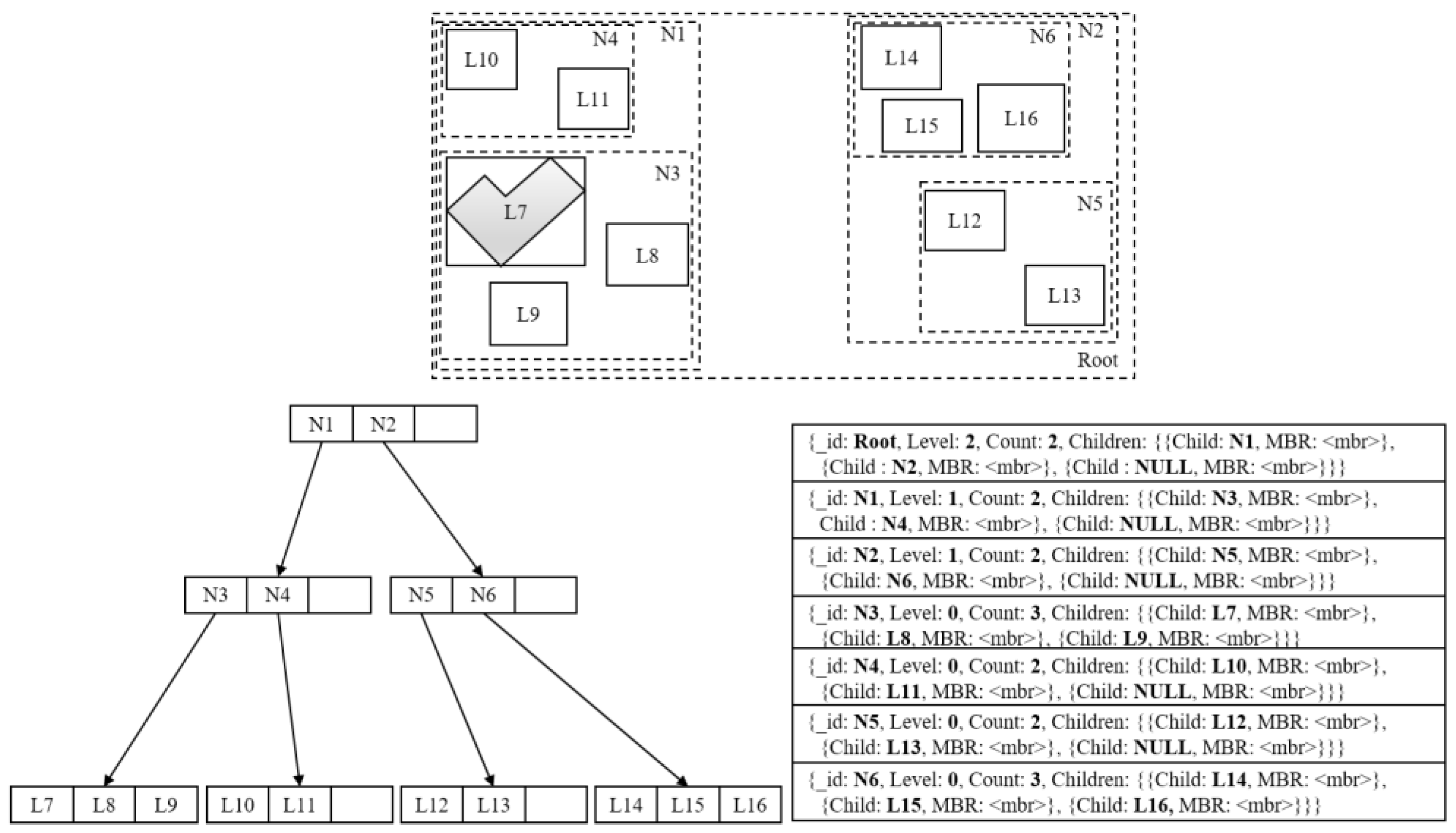
On one hand, R-tree nodes, either leaf nodes or inner nodes, are of nested structures, and R-tree pointers from parents to children are actually addresses, each indicating a unique disk location. On the other hand, MongoDB documents encoded in BSON format support a powerful mechanism to model objects with complex structures, and each MongoDB document is assigned with a unique identifier, i.e., “_id”. This motivates us to simulate R-trees with MongoDB collections and, therefore, enables MongoDB to manage planar spatial data. To be specific, an R-tree structure is presented as a MongoDB collection, where nodes are expressed as documents and pointers are substituted by document identifiers. With such a simulation, an R-tree of hierarchical structure is flattened into a MongoDB collection of tabular presentation. Consequently, a pointer-based node navigation in a hierarchical R-tree is transformed into an identifier-based document tracking in the corresponding collection and, therefore, an R-tree path directed by pointers can be represented as a string of documents linked by identifiers. Figure 1 illustrates an example of R-tree flattened with MongoDB collection, where the bottom left R-tree indexes 10 spatial objects (i.e., L7-L16) depicted in the top and the bottom right collection is the flattened result.

One can see that each collection document that exactly presents an R-tree node is designed to contain four key-value pairs. The first one represents the node identifier that uses the built-in document identifier, i.e., “_id”. The second one indicates the node level counting from leaves to the root. The third one implies how many index entries in a node are put into use. The last one specifies entry information, in which the value component is declared as an array of index entries. For each index entry I, it further contains two fixed key-value pairs: “Child” is used for document referencing while “MBR” stores a value of type MBR. If the node of I is a leaf, “Child” points to an actual spatial object stored as a document in another collection and “MBR” records the MBR of this object, otherwise, “Child” references the document corresponding to the child node of I and “MBR” calculates the MBR for all spatial objects in the branch of I. For example, the third index entry of the first document is declared to have a value “NULL” for key “Child”, implying that this entry is not used yet and, therefore, the corresponding branch is currently empty.

Though MongoDB supports schema-free data storage, we still explore a fixed structure for documents in the R-tree collection, because space pre-allocation can avoid constantly moving data on the hard disk during node expansion and shrinking [28]. In other words, all documents are created with “Children” having a maximum number of index entries, though the number of actual index entries is usually less than that. In addition, an MBR is kept for each used index entry in a node document, so that irrelevant entries can be quickly filtered out without the need to access descendants when performing queries. Finally, “Count”, serving as a redundant short-cut pair, can avoid frequent scanning through “Children” during the stage of R-tree re-balancing.

3.2. R-Tree Related Schema

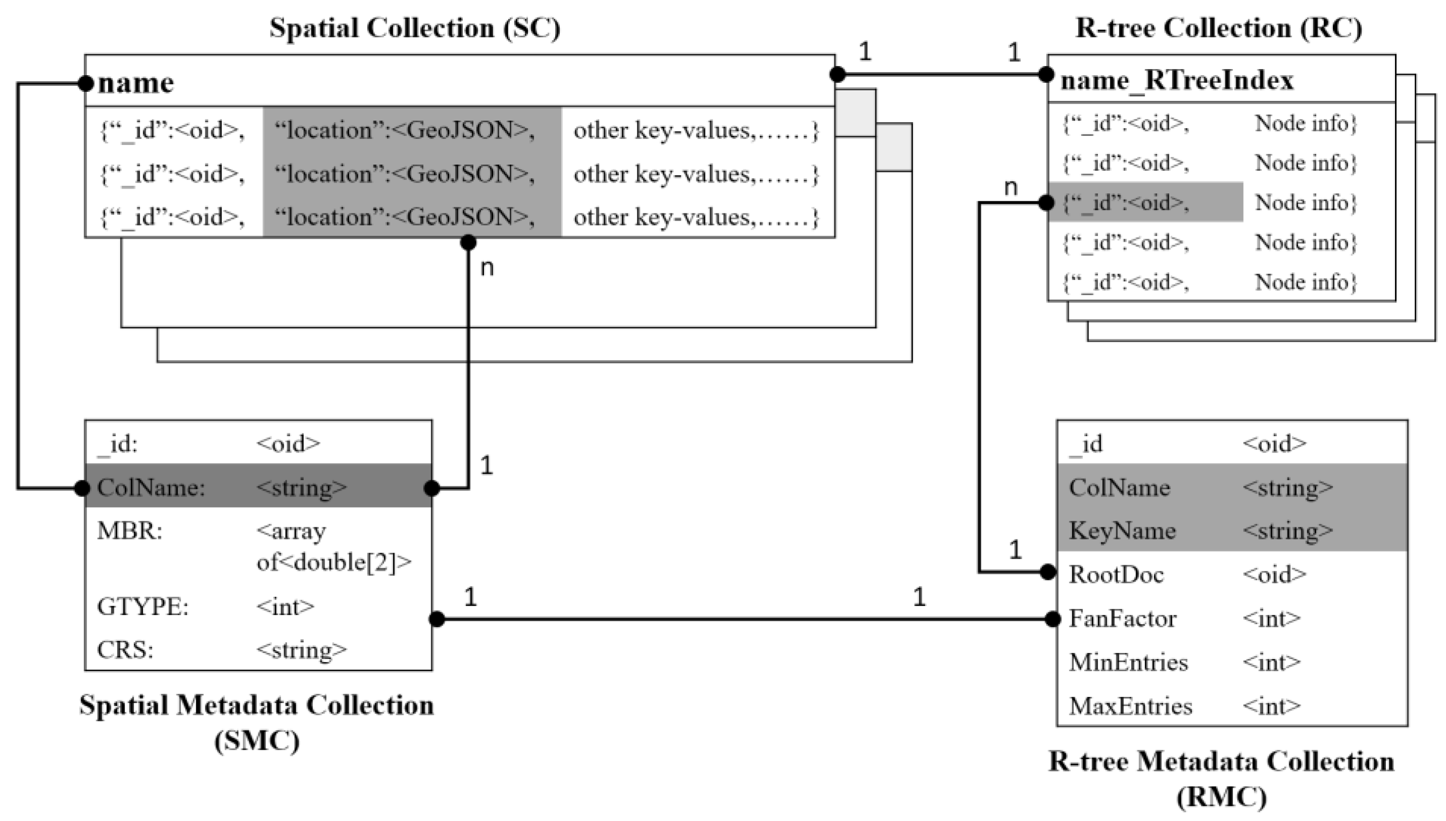
There are four kinds of collections that are involved in the management of planar spatial data, as shown in Figure 2. They are the spatial collection (SC), the R-tree collection (RC), the spatial metadata collection (SMC), and the R-tree metadata collection (RMC). With the latter two, each is allowed to have a single instance in the system, while with the former two, each can have multiple instances. Further, SC and RC form a 1:1 relationship, i.e., a spatial collection is configured with an R-tree collection.

SC is an ordinary collection with a key-value pair to store spatial data encoded in the format of GeoJSON, along with other key-value pairs to describe non-spatial attributes. RC is an auxiliary collection with a particular structure to flatten R-trees as presented in the above section. If a spatial collection is arranged to be indexed by R-tree, an R-tree collection should be created and named by appending a suffix of “_RTree” to the spatial collection’s name. Under this naming rule, one could easily identify and operate the R-tree collection for any given spatial collection. Given a planar spatial dataset, its metadata is store in SMC, and if it is indexed by an R-tree, its parameters are then recorded in RMC.

With SMC, users could tell how many planar spatial datasets, each corresponding to a SC, are managed in the system, and further acquire metadata for a registered dataset, such as its geometry type, bounding box, coordinate system, and so on. Since RMC contains a foreign key named “ColName” referencing SMC, users could track whether a spatial collection is R-tree indexed or not by a join operator. Hence, R-tree metadata, like target key (on which the R-tree is built), root document and branching factor, is also available to users. Note that in SMC: key “MBR” is a multi-dimensional bounding box, not just limited to a 2D space, key “GTYPE” should be one of the seven native geometry types supported by GeoJSON, and key “CRS” takes a valid spatial reference system identifier under the EPSG (European Petroleum Survey Group) framework.

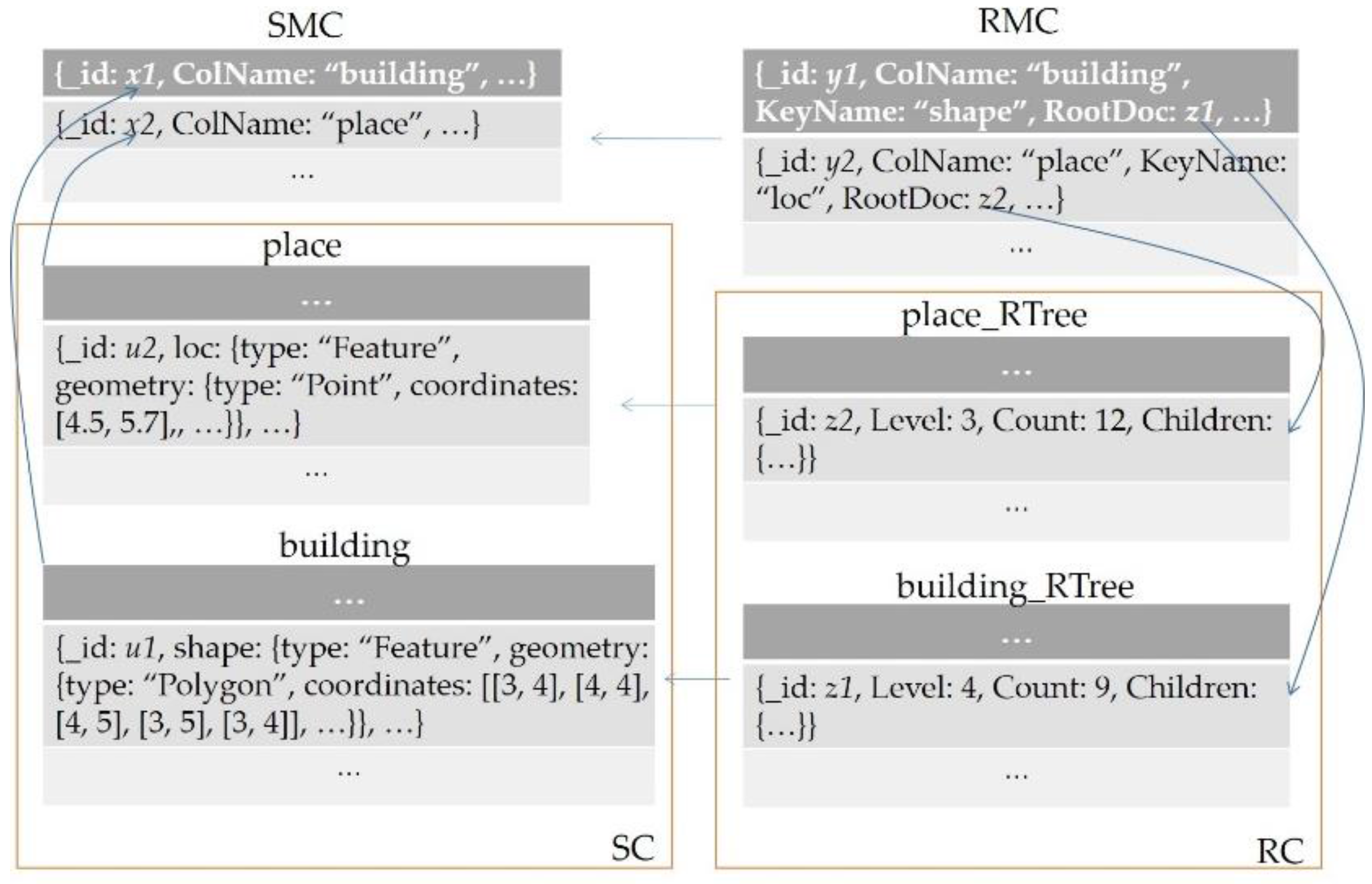
In order to illustrate the R-tree-related storage schema, a user case about spatial data in a city is presented in Figure 3. One can see that two spatial datasets have been loaded into the database as two collections (“place” and “building”) in the namespace of SC and registered in SMC as two documents (x1 and x2). In addition, R-trees for the two datasets have been created in the namespace of RC, namely “place_Rtree” and “building_RTree”, and their metadata have been saved in RMC, namely y1 and y2. With this user case, one could easily derive from SMC that there are two spatial datasets available in the database. Further, it could be confirmed from RMC that each of them is accompanied by an R-tree.

4. Integrating R-Tree into MongoDB

4.1. Framework and Workflow

There exist two strategies for MongoDB to integrate flattened R-tree: an agency to shield MongoDB and a module to plug into MongoDB. The former serves as a middleware between the client and database and, therefore, is relatively easy to be implemented, however, it will increase the learning cost of end users who might have to be familiar with a new tool and master a new script language. Hence, we chose the second integration option that allows users to use a flattened R-tree in almost a same way as the built-in 2dsphere.

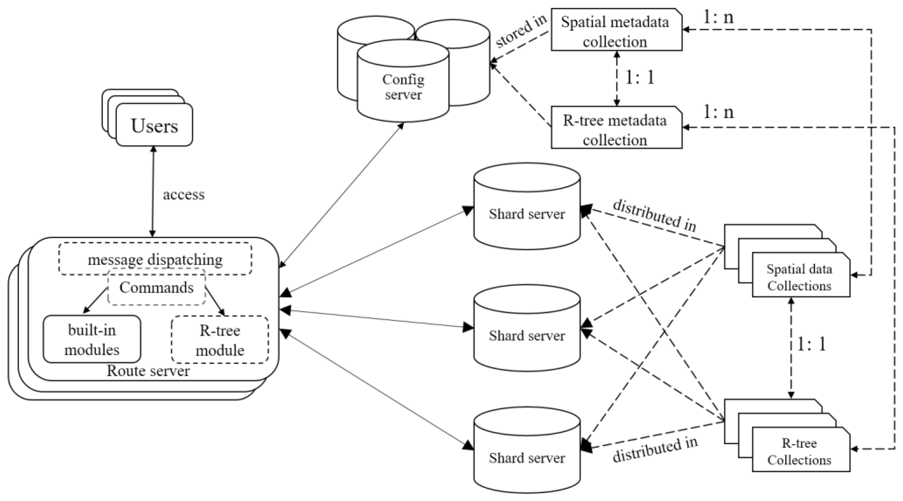
The MongoDB-based R-tree integration framework is presented in Figure 4. The right part depicts the configuration of R-tree storage schema and the left part shows how R-tree is embedded into MongoDB. One can see that SMC and RMC, serving as metadata, are stored in the config server, while SC and RC may be distributed across all nodes in shard server by enabling the sharding function on document identifiers. It means a flattened R-tree, if necessary, can distribute its nodes among different storage nodes and, therefore, the I/O efficiency of R-tree access will be shared, which will obviously benefit query processing, especially for concurrent queries.

The R-tree module is implemented and deployed in router server, which supports CRUD operations by manipulating SMC and RMC in the config server as well as SC and RC in the shard server. Similar to 2dsphere, R-tree supported CRUD operations are encapsulated into commands that inherit from the root system command. Users could issue a command in the format of GeoJSON, which are then packaged as a network message of binary structure, and finally sent to the router server. At the entrance of the router server, the function of message handling is rewritten, which first parses the received message, re-constructs the corresponding command, and then dispatches it to the R-tree module or built-in modules for execution. To be specific, if a command is targeted to a planar spatial data, it will go to the R-tree module to invoke a newly-derived command, otherwise it will go to built-in modules to execute some native command. Suppose command {$geoIntersects: {$geometry: {type: “Polygon”, coordinates: [[100, 100], [150, 100], [120, 140], [100, 100]]}}} is issued against “city.place.loc”, where “city” indicates a database, “place” is a collection in “city”, and “loc” is a spatial field in “place”. Obviously, this command encapsulates a read operation of overlap searching, which will be executed by the R-tree module if an R-tree has been built on field “loc” of collection “place” in database “city”.

Figure 5 presents a typical workflow for R-tree supported operations, in which the involved steps are depicted by circled numbers. After the route server receives and then parses a network message (step 1), our codes implanted in the message handling will consult with the config server to check if a flattened R-tree is created for the target collection (step 2), and in the yes case, a proper command provided by the R-tree module is pinpointed (step 3). Then, the corresponding SC and RC is queried and/or maintained by forming a series of native commands (step 4) and sending them to the shard server (step 5). Next, the shard server executes commands locally and replies to the R-tree module with the results (step 6). If necessary, the results returned from the route server will be refined (step 7). Finally, the qualified results are packaged as network messages and sent back to user (step 8).

4.2. Two Key Issues

(1)

I/O detached design of R-tree

The flattened R-tree is designed to consist of two levels of loosely-coupled components, as shown in Figure 4. The ground level provides an I/O interface based on the unit of document, taking charge of operating four kinds of collections; the ceiling level supports various R-tree algorithms, namely search, insert, delete, and update, as well as provides functions to operate two metadata collections and, therefore, taking charge of searching/maintaining the flattened R-tree. Consequently, the ceiling level becomes storage-independent, focusing on R-tree logic, while the ground level concentrates on data exchange. Although this I/O-detached R-tree is developed for the document-oriented MongoDB database, it can be easily ported into other storages, like file systems, by overwriting the I/O interface.

In order to further improve the I/O efficiency, the R-tree module is configured with a cache to keep frequently-used node documents in memory. Here, we adopt the LRU method as the replacement strategy to discard the least recently used R-tree nodes. As R-tree nodes are simulated by MongoDB documents that are fixed in size, and each of them carries a unique identifier, this node-based caching is simple in structure, easy to manipulate and, consequently, the amount of document fetching through the I/O interface can be significantly reduced.

(2)

Reusing and extending of system commands

Similar to 2dsphere, the R-tree module communicates with the function of message handling through commands inherited from the root command in router server’s command system. Further, commands that operate 2dsphere are reused on the R-tree as much as possible in order to introduce as few new commands as possible.

Table 2. Main commands supported by the R-tree module.

Command	Type	Involved Native Commands
		Find	Insert	Update	Remove
registerGeometry	new	√	√
createIndex	overridden	√	√
find	overwritten	√
insert		√	√	√
update		√	√	√	√
remove		√	√	√	√

summarizes the main commands supported by the R-tree module. Note that a command called “registerGeomtry” is added to identify collections used to store planar spatial data and their metadata, and consequently, the common layer concept is brought into MongoDB to manage planar spatial data. In addition, “createIndex” is an overridden command because R-tree asks for parameters different from 2dsphere, while others are all overwritten commands over their native ones. This means an overwritten command, e.g., find, shares the same declaration of both name and arguments with its native one, but its implementation is targeted on the flattened R-tree structure. With our command design, planar spatial data can be manipulated by the flattened R-tree through almost the same set of commands as geodetic spatial data with 2dsphere.

As mentioned in the last subsection, a set of native commands will be involved when executing an R-tree command, the details of which are presented in Table 2. For example, “registerGeometry” first calls “find” to test if a document already exists in SMC with the same name, and then in the no case, calls “insert” to write a document into SMC. By transforming an R-tree command into a series of native commands, the R-tree module achieves performing various logic operations without the need to know how data and metadata are configured and distributed among the MongoDB clustering.

5. Managing Planar Spatial Data with Flattened R-Trees

5.1. CRUD Operations

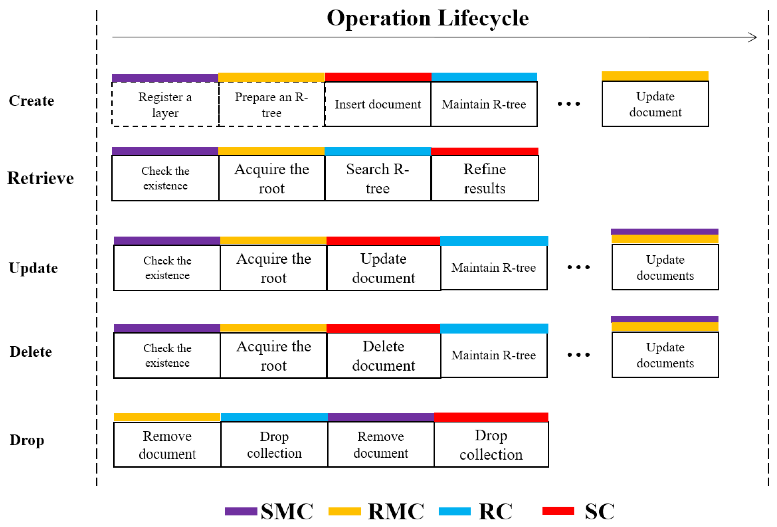
CRUD operations, including create, read, update and delete, are the basic functions that a database or a persistence layer should support. In Figure 6, the execution logic with the flattened R-tree for CRUD operations, as well as for the drop operation, is presented. Note that each operation is carried out by a series of commands, either an R-tree command or a native command.

Given a planar spatial dataset, a task of priority is to load it into MongoDB as a layer with the create operation, which involves three consecutive R-tree commands. Firstly, “registerGeometry” is called to register a spatial layer in SMC, then “createIndex” is called to record an R-tree in RMC and, finally, “insert” is called multiple times to populate geometries into SC and build a flattened R-tree in RC. The last command is somewhat complicated for each time “insert” is called; it will write a document into SC, append an entry into RC, maintain the structure of RC and, if a new root document is created, update the corresponding document in RMC. For better data protection against unseen accidents, like system crashes, it is important to ensure that SC writing should be carried out before RC updating, because a RC can be restored by scanning its SC, but not the opposite.

The retrieve operation simply calls the R-tree command “find”, during which a three-step strategy is explored. The first step is to verify the existence of target spatial layer and flattened R-tree in SMC and RMC, respectively, and if it exist, the document identifier of the root node is acquired from RMC. The second step is to filter, which navigates the flattened R-tree from the root document to leaf documents and excludes branches whose MBRs are not intersected with the input range. As a result, a set of candidate documents is obtained which will then go through the final step, i.e., refining with accurate geometry. After that, the final result is returned. Note that the refining step uses Cartesian computation powered by GEOS [28], a well-known open source geometry library.

A delete operation can be finished just by calling the R-tree command “remove”, which involves SC deleting and RC updating. Unlike “insert”, “remove” firstly runs RC updating to maintain the R-tree and then performs SC deleting to remove documents, thus avoiding empty referenced entries in leaf documents. In addition, if the delete operation causes a new root node or a shrunken layer MBR, the native command of “update” will be called to update RMC or SMC. Similarly, the update operation can be implemented. In order to maintain flattened R-tree under “update”, a commonly used re-insert strategy [19] is adopted. Finally, a drop operation is used to drop a planar spatial data layer, including its data and metadata. Therefore, it first deletes a document from RMC with a native “remove”, then drops the RC with a native “drop”, and finally processes SMC and SC in a similar manner.

5.2. Query Processing with Cursors

In this subsection, query processing with cursors based on the flattened R-tree structure, including range and near queries, is discussed in some detail. Consider a query that has a result of large numbers of records, cursor-enabled processing allows the result to be returned in batches and, therefore, users could browse and analyze qualified records as quickly as possible, without the need to wait a long time for the whole result. For that reason, the cursor has become an essential configuration for answering queries in modern database systems and data-related applications. In order to add cursor support for range queries, RC is searched by a depth-first traversal: every time a leaf entry le is scanned and then validated as a qualified item, the document that le points to will be pushed into a queue with a fixed number of entries. When the queue is full, it is returned to the user as a partial result and, in the meantime, the searching of RC is suspended. Then, the user could move forward the query-associated cursor to trigger the next round of fetching, which will first prepare an empty queue and then resume the searching procedure.

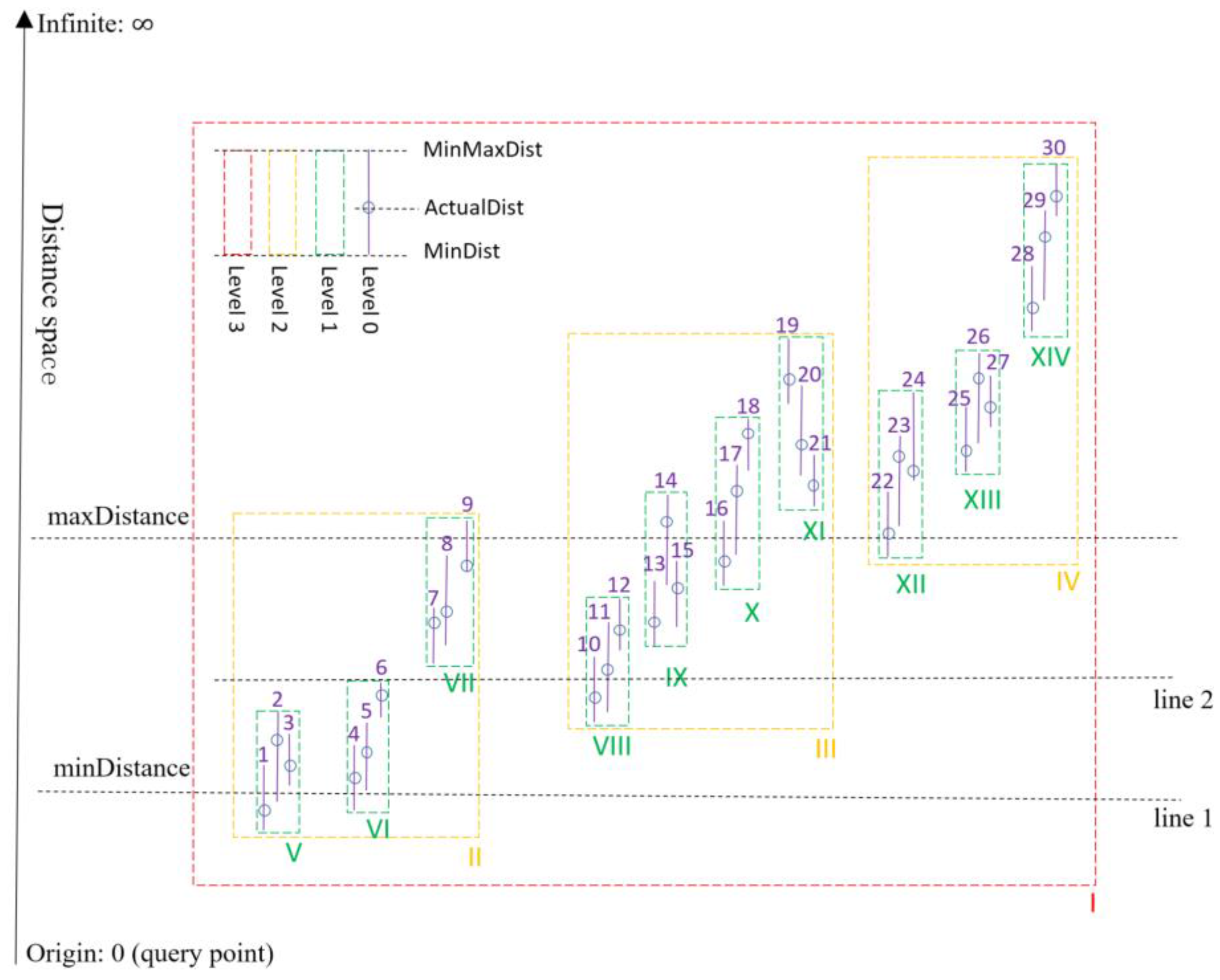
Near queries, compared with range queries, are much more complicated to be handled. As far as static spatial objects are concerned, the most powerful method for k-nearest neighbor searching, to the best of our knowledge, is the incremental nearest neighbor algorithm [29]. Note that flattened R-trees reside in MongoDB which issues near queries with the following command: {$near: {$geometry: {type: “Point”, coordinates: [<longitude>, <latitude>]}, $maxDistance: <distance>, $minDistance: <distance>}}. 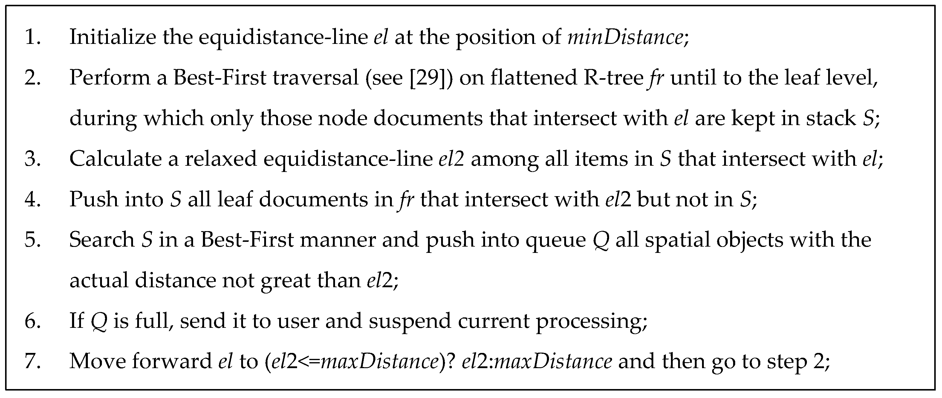Obviously, near queries supported by MongoDB try to look for sorted spatial objects with the distance to the queried point falling into [minDistance, maxDistance]. By putting a distance constraint and testing it during searching, the incremental algorithm could adapt to the MongoDB environment. However, such modification, though straightforward, is inefficient, so that a more efficient variant with cursor support based on the flattened R-tree structure is developed, the pseudo-code of which is presented in Figure 7.

Figure 8 depicts the distribution graph of an example R-tree in the distance space with respect to a query point, which will be explored to illustrate how to handle a near query with the above algorithm. For the first round of scanning (assuming el is at line 1), nodes V and VI are determined in step 2, el2 located at line 2 is derived in step 3, and node VIII is joined into S in step 4. After that, the three involved leaf nodes will be expanded in a best-first manner [29], and consequently, objects 4, 3, 5, 2, 10, and 6 will be pushed into Q gradually. The last step is to move forward the equidistance line to line 2, from which a next round of scanning could be performed. The main idea behind the algorithm of Figure 6 is to move forward the equidistance line from minDistance to maxDistance, during which related nodes and entries are progressively scanned and processed. Compared with the straightforward modification, our variant reads and checks as few node documents as possible to return the result in batches and, therefore, achieves to answer MongoDB near queries in a more efficient way.

6. Experimental Evaluations

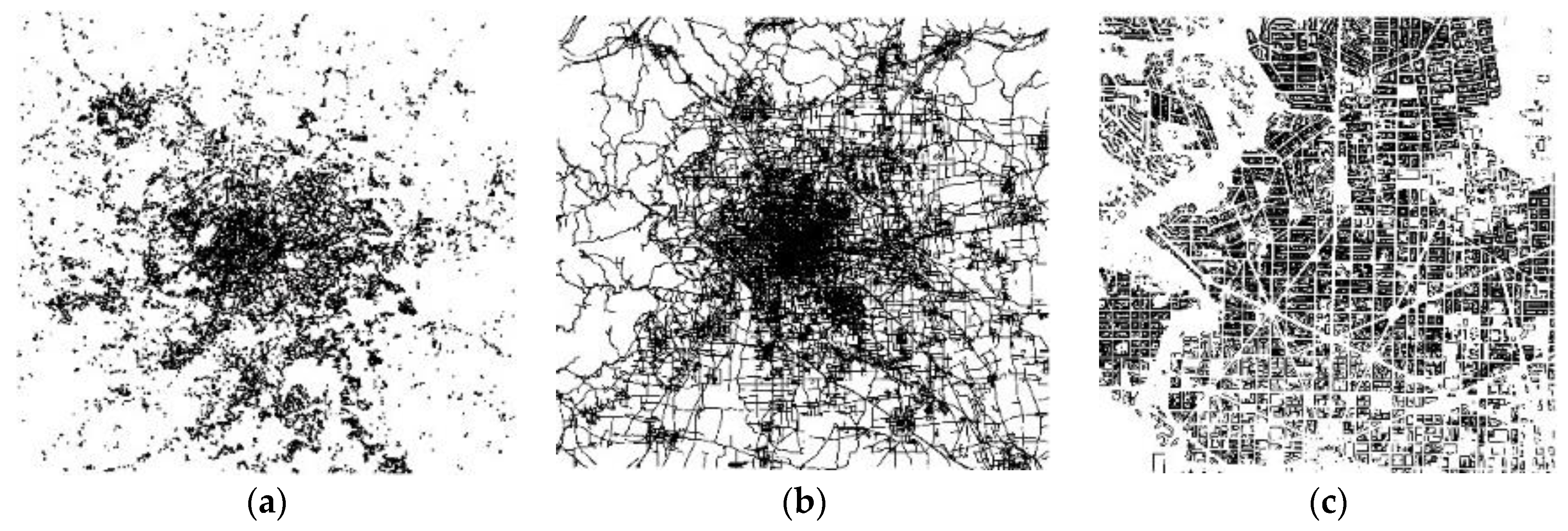
Among CRUD operations, create and read, compared with update and delete, are much more frequently used and performance-sensitive under the context of spatial applications, so that, in this section, the evaluation of the R-tree module is designed and discussed from two perspectives: structure construction and query processing. Three datasets with diverse coverage, types, and sizes were inputted to test the performance of our MongoDB R-tree implementation. These datasets were downloaded from the OSM website (Open Street Map, www.openstreetmap.org), and then projected under a Cartesian coordinate system. As a result, each dataset has two versions: one is geodetic and the other is projected.

Table 3. Three experimental datasets.

Dataset	Geometry Type	Area	Feature num.
Paris POI	point	78 km × 72 km	24739
Beijing street	line	123 km × 113 km	59192
Washington DC building	polygon	20 km × 20 km	173746

presents details of the three datasets, while Figure 9 shows thumbnail images of the three datasets.

The version of MongoDB chosen to integrate the flattened R-tree is 3.2.0. All experiments have been carried out on a PC running Windows 10 with Intel Core i5-4200H 2.8GHz CPU and 16GB RAM, in which a simplest MongoDB cluster composed of one shard instance, one config instance, and one route instance (including the R-tree module) was configured. The test program that issues commands exposed by the R-tree module ran on the same machine.

6.1. Construction of Flattened R-Trees

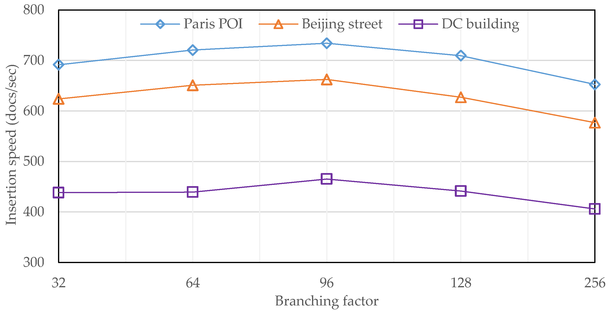
This experiment aims at evaluating the efficiency of R-tree construction, during which five flattened R-trees with different branching factors were constructed for each projected dataset. The results, measuring the number of inserted documents per second, are presented in Figure 10. From the horizontal point of view, the three performance curves exhibit a very similar appearance on both shape and trend. On one hand, as the branching factor increases from 8 to 256, the insertion speed initially increases, but turns to decrease after reaching a maximum at the branching factor of 96, because the size of an R-tree node with 96 entries is mostly close to that of a disk page (namely 4096 bytes). On the other hand, the overall fluctuation is relatively small because of the two levels of caching, i.e., built-in structure caching in the shard server and developed node caching in the R-tree module.

From the vertical point of view, the insertion speed of the third dataset is significantly slower than that of the other two datasets, because the third dataset has a higher density on object distribution and, therefore, it is more likely to trigger node overflow during R-tree construction. In addition, the first dataset achieves a highest insertion speed due to its geometry type of point.

Finally, we also built a 2dsphere index on the geodetic version of the third dataset and the recorded runtime is about 230 s, which means the insertion speed is about 755 docs/sec. It is remarkably higher than that of flattened R-trees, just because 2dsphere is actually a kind of B⁺-tree with a much simpler structure compared with the R-tree and, therefore, it needs less time to be built.

6.2. Query Processing with the Flattened R-Tree

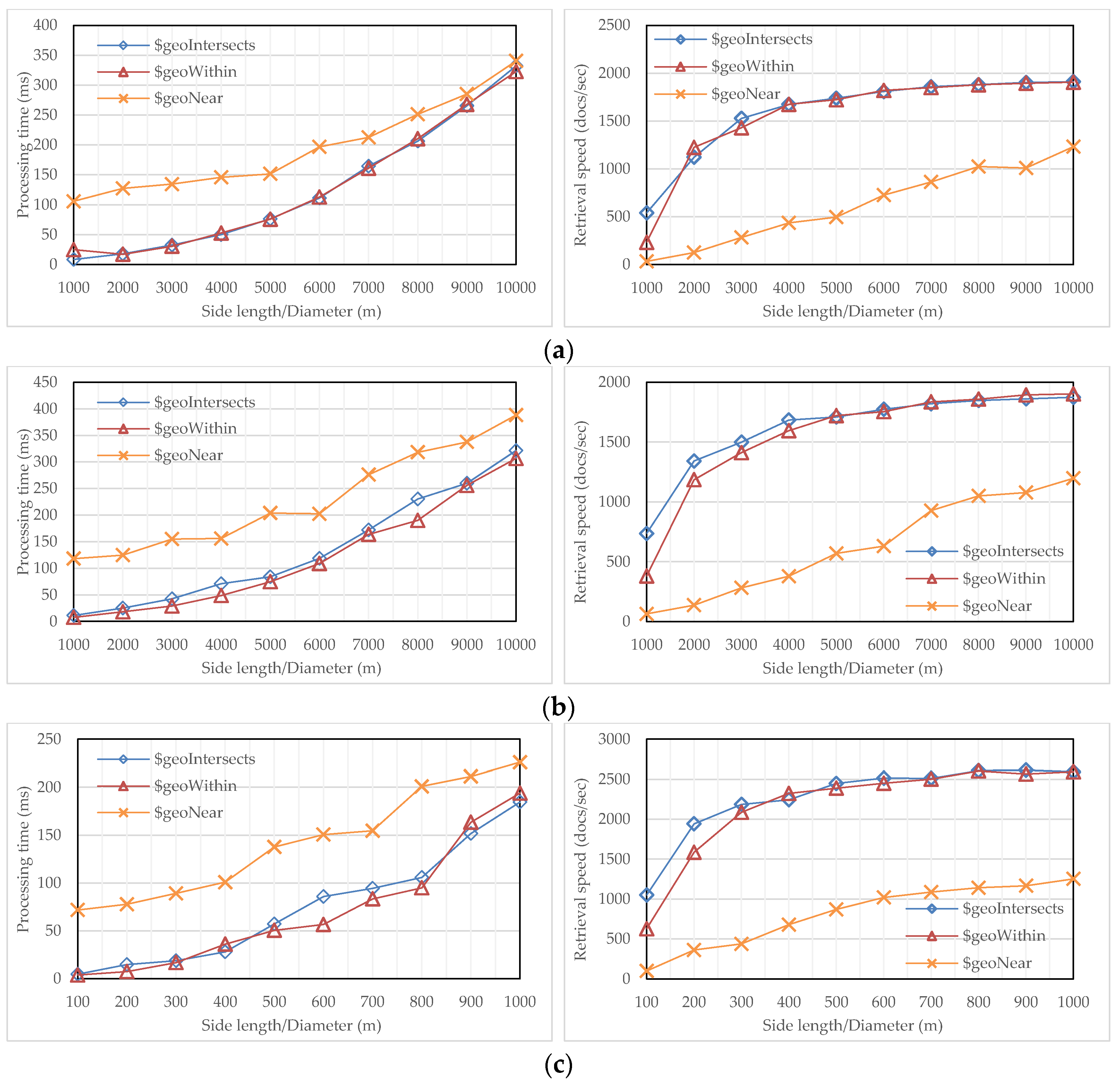
In order to derive the performance of query processing with the flattened R-tree, each dataset was tested with three different MongoDB-supported predicates, i.e., $geoWithin, $geoIntersects, and $near. The predicate of $geoWithin retrieves objects that are wholly contained within a query window; the predicate of $geoIntersects retrieves objects that overlap with a query window; the predicate of $near first fetches objects that fall into a specified distance interval with respect to a query point, and then output them in an order from nearest to farthest. Before testing, a group of square windows with random center positions and different side lengths were prepared for $geoWithin and $geoIntersects, and a group of circles with different radii, but centered at a fixed point, were generated for $near. One generated query for the first dataset is: “test.paris.find(loc: {$geoWithin: {$geometry: {type: “Polygon”, coordinates: [[449263, 5407890], [450263, 5407890], [450263, 5408890], [449263, 5408890], [449263, 5407890]]}}})”, which will issue a command for a read operation with the predicate $geoWithin.

During each test, the flattened R-tree with a branching factor of 96 was selected to accelerate query processing. The results are presented in Figure 11, in which every dataset is measured from two perspectives, one processing time and the other retrieval speed. From the viewpoint of predicates, $geoWithin and $geoIntersects perform very similarly over the three datasets on not only processing time but also document throughput. As the query window enlarges, the response time increases dramatically, while the throughput initially increases, then tends to stabilize. For example, the retrieval speed of the third dataset starts at about 1000 docs/s, then keeps increasing, but finally stabilizes at about 2500 docs/s. By comparison, it is less efficient for $near to be processed with the flattened R-tree, but the gap continuously shrinks as the query window enlarges. The reason is that $near performs searching as well as ranking: with a small query window, ranking accounts for a high share of the runtime; while inputting a large query window, searching, due to involving a substantial amount of I/O, dominates the runtime. In addition, the document throughput of $near keeps increasing, though the growth tends to be narrowed.

From the viewpoint of datasets, all three predicates perform much better over the third dataset on both processing time and retrieval speed. For example, the retrieval speed of first two datasets is less than 2000 docs/s, while it reaches to about 2500 docs/s over the third dataset. This is because the first dataset is actually a road network with a line type geometry, leading to a high degree of MBR overlapping in its R-tree, while the second dataset has an uneven distribution of objects, leading to a high degree of dead space in its R-tree. By comparison, the distribution of objects in the third dataset is remarkably even, an ideal situation for R-tree to process queries.

6.3. Comparison with 2dsphere on Query Processing

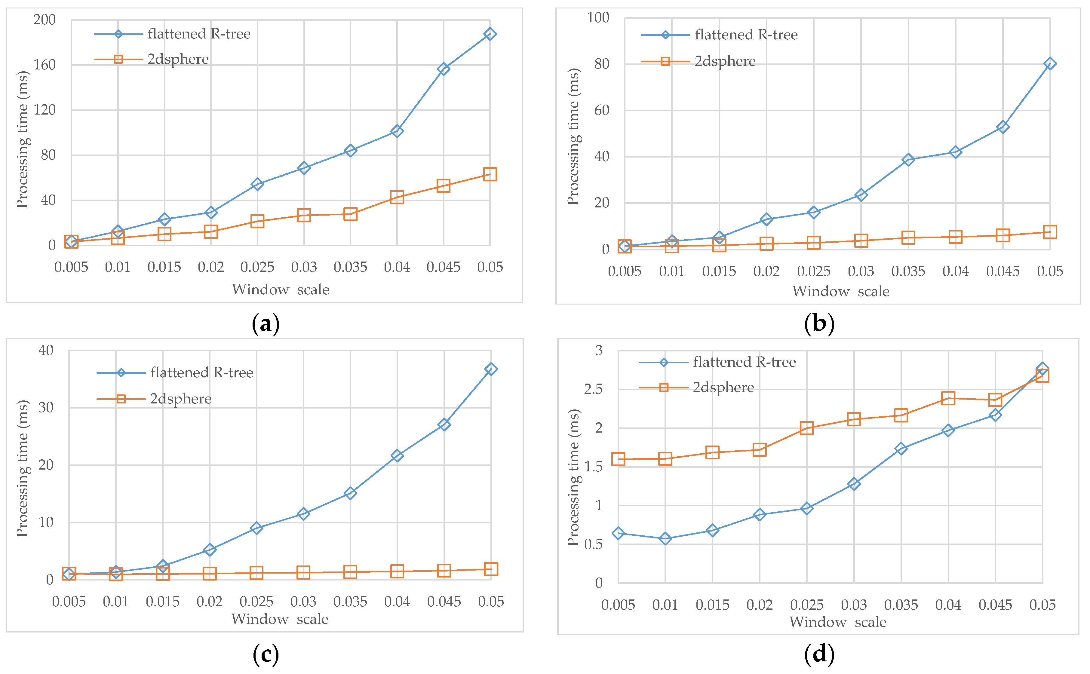
Finally, the query processing of the flattened R-tree was compared with that of 2dsphere. A group of query windows scaling from 0.5% to 5% over the whole input area were generated for each dataset, including both geodetic and projected versions, and then a mixture of $geoWithin and $geoIntersects was prepared for each query window. The runtime took the average. The results are presented in Figure 12a–c.

Obviously, 2dsphere performs much better than the flattened R-tree over the three datasets, and the gap becomes larger and larger as the window size increases. The reason is two-fold: (1) computation and storage are separated on two different MongoDB instances (and may be distributed on different physical nodes) for the flattened R-tree while they are coupled together in a single MongoDB instance for 2dsphere, which means 2dsphere is more efficient on data access; and (2) most objects in the three datasets are of small sizes (note: the roads in the dataset of the Beijing street data are actually segments linking intersections), which means each object could be approximated by one or a few of cells, so that not only the resulting 2dsphere is relatively simple in structure, but also the geometry calculation over objects becomes efficient. One may observe that the advantage of 2dsphere against the flattened R-tree is more remarkable on the dataset of Paris POI, because this dataset has a point type geometry and, therefore, all objects are exactly approximated by single cells.

In addition, this experiment was repeated on the lake dataset of Wuhan, China that contains 4260 polygon objects, and the results are presented in Figure 12d. With the increasing window size, our flattened R-tree initially outperforms the built-in 2dsphere but eventually catches up. The reason is that the objects in this dataset are complex in shape and vary in range (from thousands of square meters to tens of square kilometers) and, therefore, geometry calculation, particularly for 2dsphere, contributes a lot to the processing time when the query window is small or moderate, while data fetching starts to dominate the runtime when the query window becomes large.

7. Conclusions

This paper addresses how to explore MongoDB, a popular NoSQL product characterized as a document-oriented, rich query language and highly available, to manage planar spatial data that are still widely used in city-scale spatial applications. The core idea is to flatten the hierarchical R-tree structure into a tabular MongoDB collection, during which the R-tree nodes are represented as collection documents and R-tree pointers are replaced by documents identifiers. With this idea, an R-tree module for managing planar spatial data is developed and seamlessly integrated into MongoDB. R-tree-based CRUD operations are performed within the router server, while metadata is stored in the config server and data is distributed across shard server. By taking over message handling and overwriting native commands, the R-tree module achieves to manipulate planar spatial data with existed system commands in addition to one new command. Moreover, a novel algorithm based on a flattened R-tree for MongoDB near queries is developed to support cursor-navigated result-fetching. The experimental evaluation with real-world datasets varying on coverage, type, and size, shows that the MongoDB-based flattened R-tree succeeds in managing planar spatial data and performs well on query processing, especially for complex and large spatial objects.

Our current implementation based on MongoDB 3.2.0 is released on https://github.com/lmars-gis/mongo/tree/v3.2.0/rtree for open access. In the near future, in addition to continuing to explore strategies and algorithms to provide consistency and recovery in case of unpredictable failures, we will investigate advanced spatial operators, like buffer and join, and eventually develop a spatial module for MongoDB to enable NoSQL technologies on spatial data. We will also consider how to push flattened R-trees into a shard server to accommodate the computation and storage of the flattened R-tree together, in which the greatest challenge is how to efficiently map spatial data and aggregate results across storage nodes.