
A Local Land Use Competition Cellular Automata Model and Its Application


Abstract
:1. Introduction
2. Data and Methods
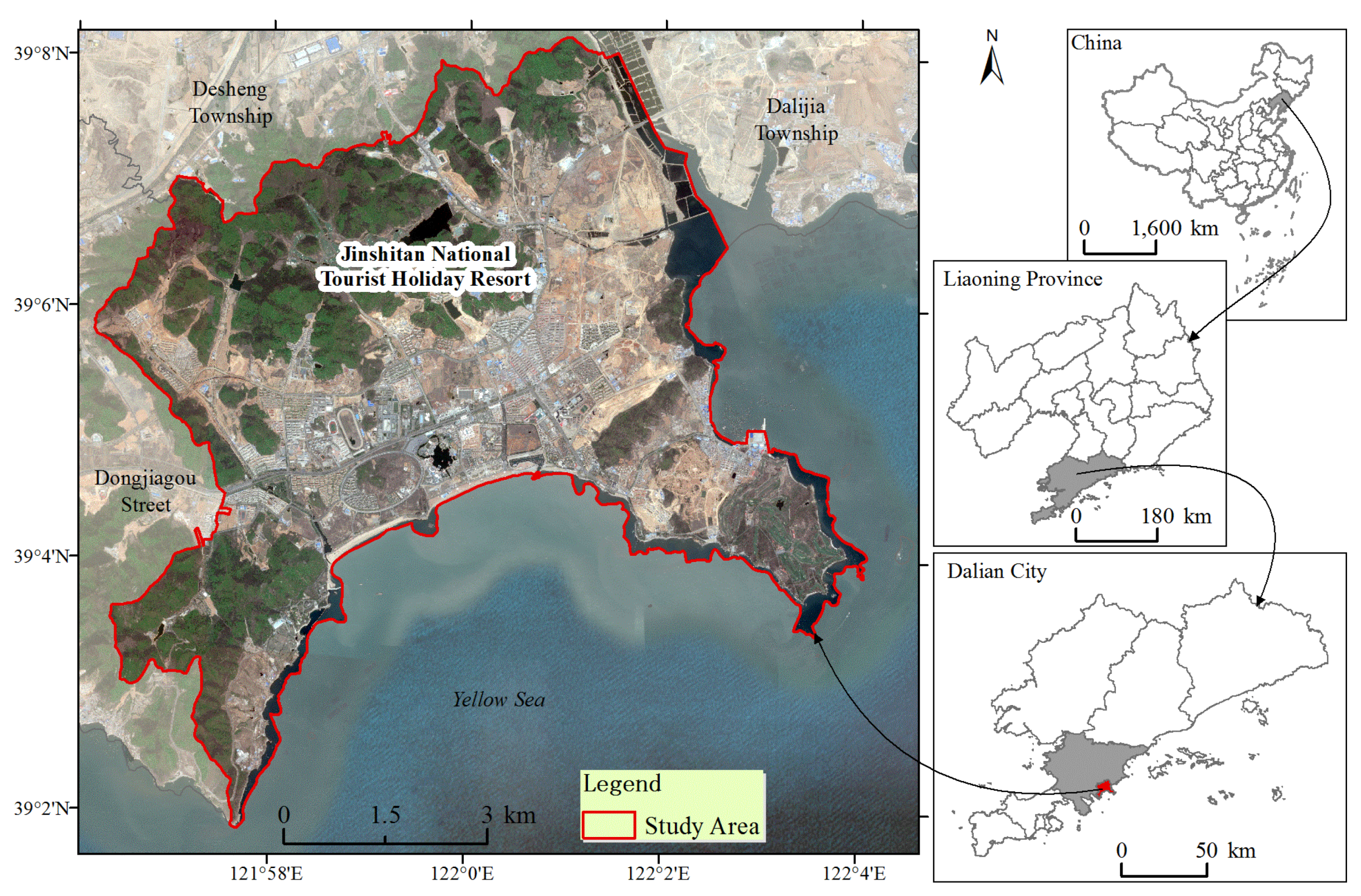
2.1. Study Area
2.2. Data Sources and Processing
2.3. The Model
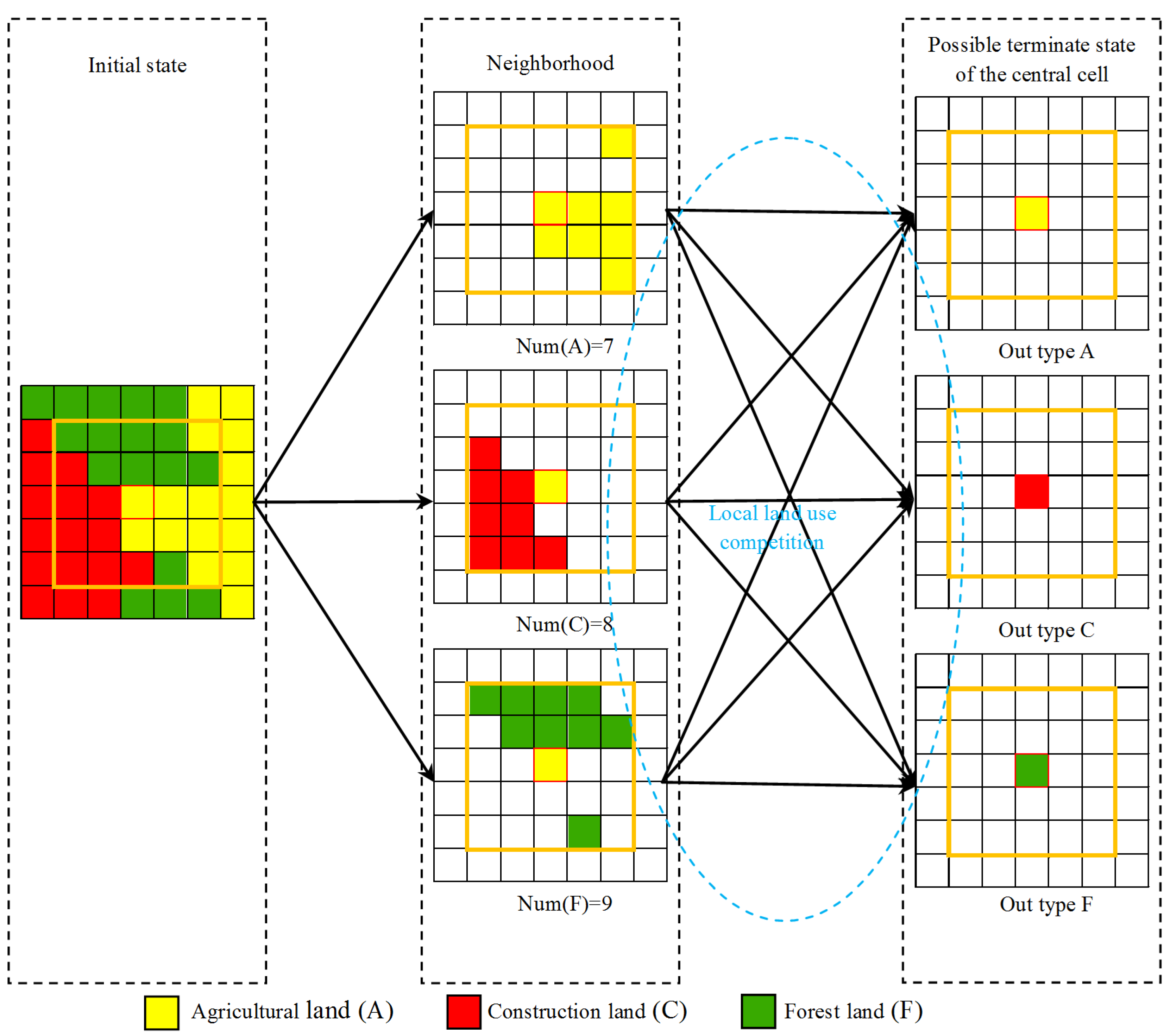
2.3.1. Local Land Use Competition
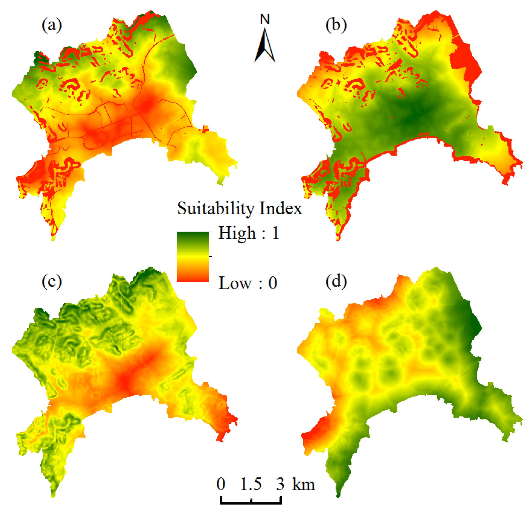
2.3.2. Land Suitability and Transition Potential
2.3.3. Demand Analysis of Different Land Types
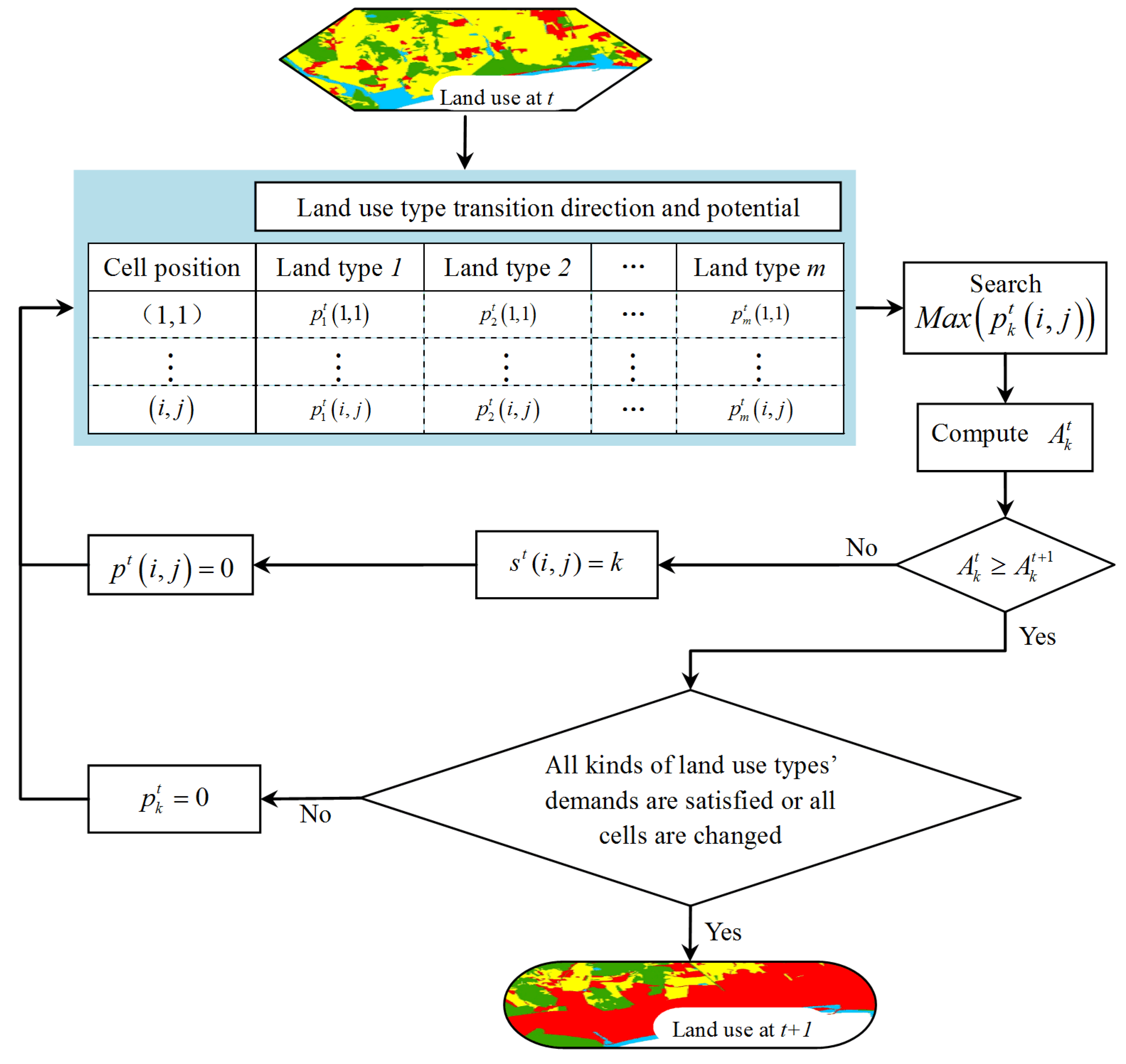
2.3.4. Multi-Target Land Use Competition Allocation Algorithm
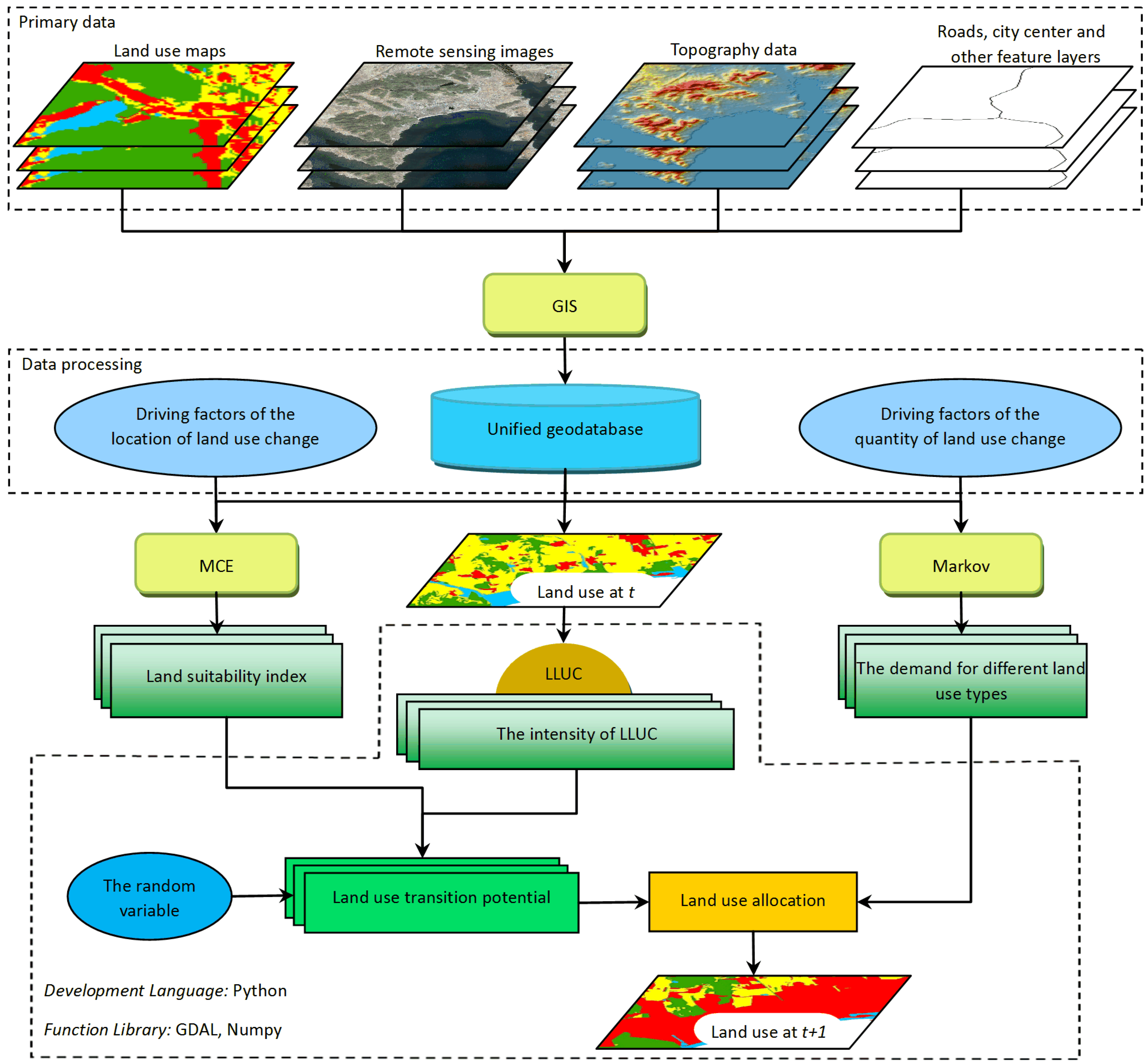
2.3.5. LLUC-CA Model Structure
2.4. Model Parameters Prepare and Implementation
3. Results and Discussion
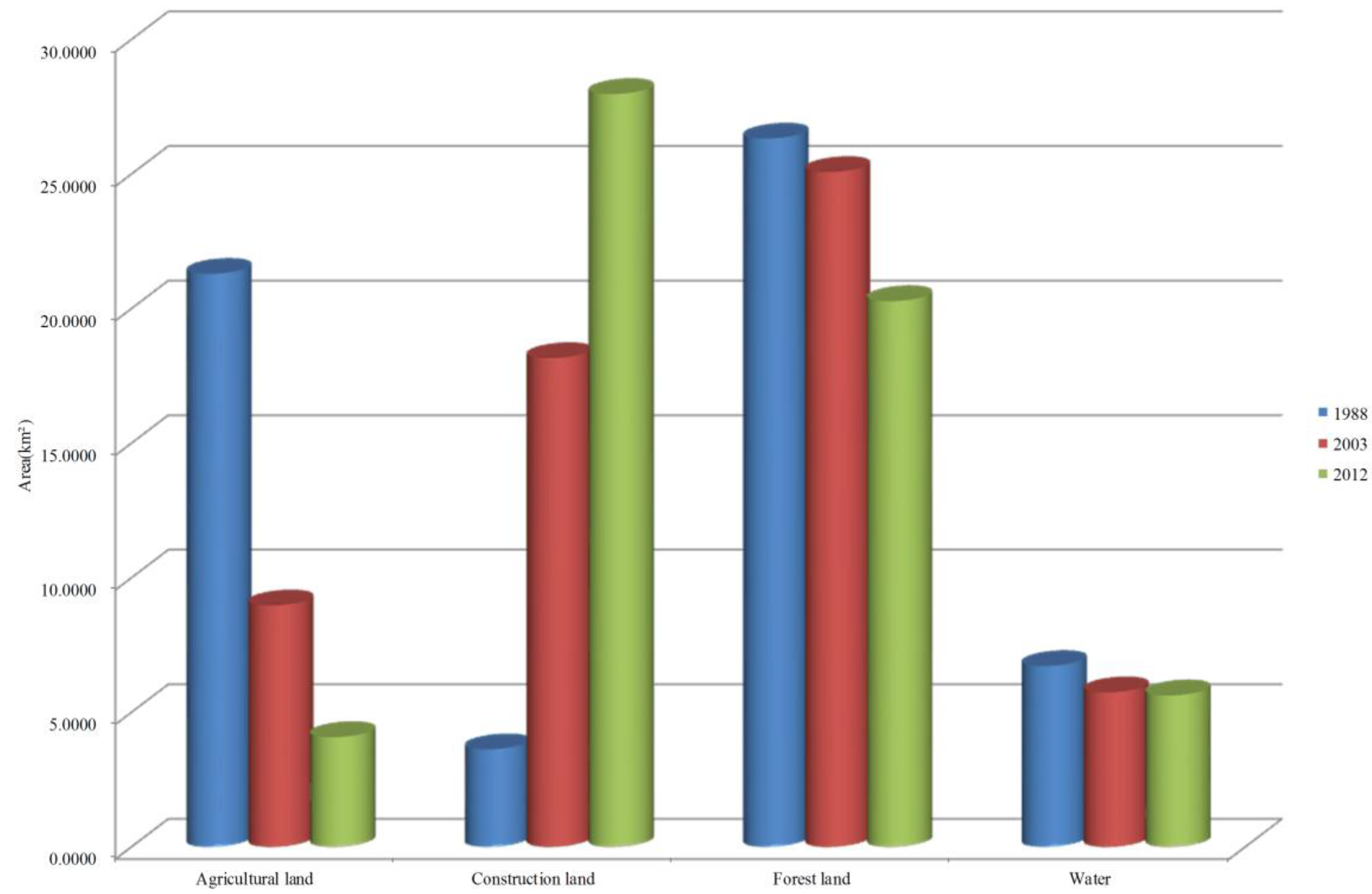
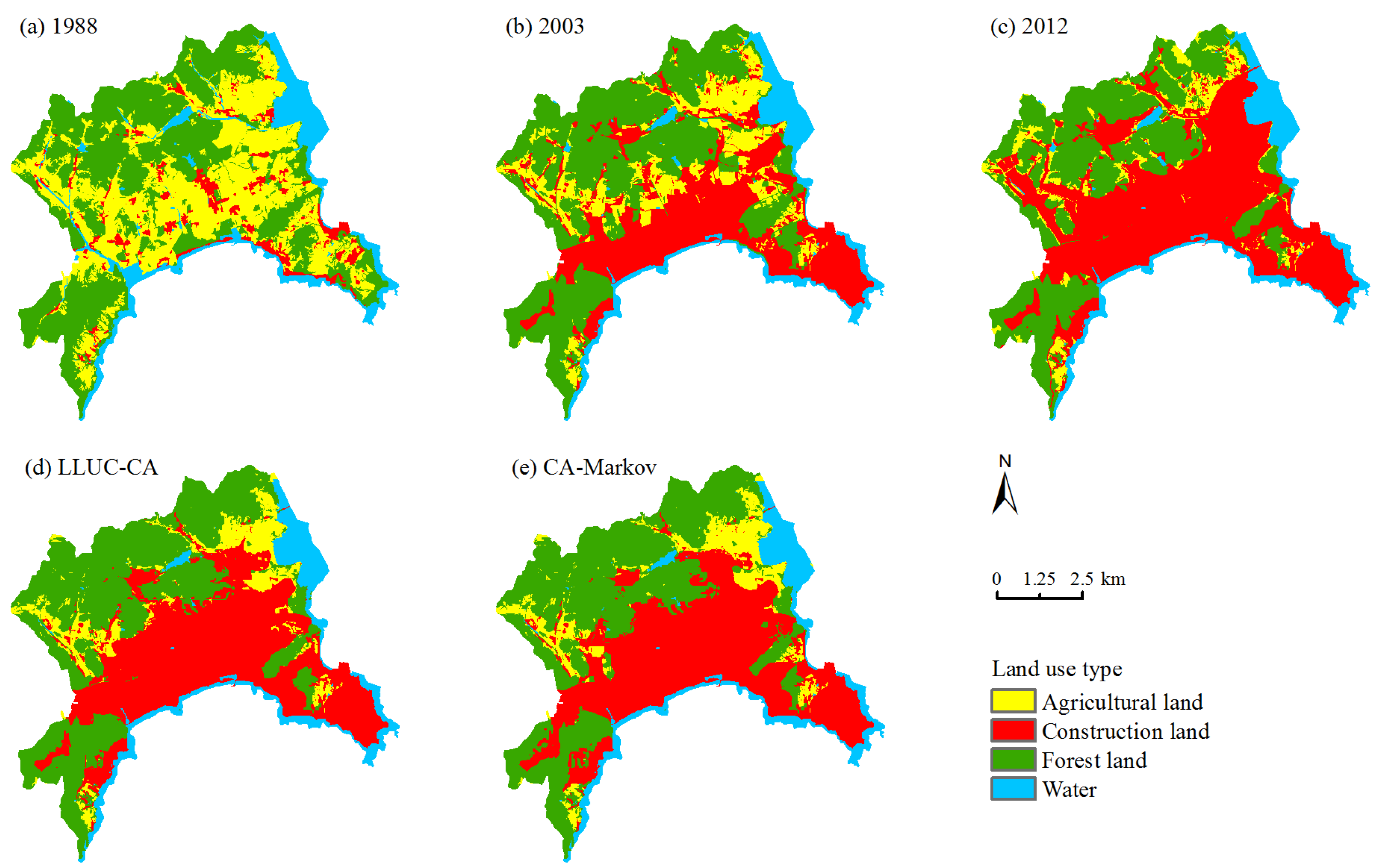
3.1. Analysis of Land Use/Cover Changes
3.2. Model Validation
4. Conclusions
Acknowledgments
Author Contributions
Conflicts of Interest
References
- Shi, P.; Gong, P.; Li, X. The Methods and Practices on Land Use/Cover Change Research; Science Press: Beijing, China, 2000. [Google Scholar]
- Rindfuss, R.R.; Walsh, S.J.; Turner, B.L.; Fox, J.; Mishra, V. Developing a science of land change: Challenges and methodological issues. Proc. Natl. Acad. Sci. USA 2004, 101, 13976–13981. [Google Scholar] [CrossRef] [PubMed]
- Li, Z.; Guan, X.; Li, R.; Wu, H. 4D-SAS: A distributed dynamic-data driven simulation and analysis system for massive spatial agent-based modeling. ISPRS Int. J. Geo-Inf. 2016, 5, 42. [Google Scholar] [CrossRef]
- Yu, B.; Lu, C. Land resource competition and land-use change in Shunyi district, Beijing. Trans. Chin. Soc. Agric. Eng. 2006, 22, 94–97. [Google Scholar]
- Lin, Y.; Deng, X.; Zhan, J. Simulation of regional land use competition for Jiangxi province. Resour. Sci. 2013, 35, 729–738. [Google Scholar]
- Huang, Q.; Shi, P.; He, C.; Li, X. Modelling land use change dynamics under different aridification scenarios in northern China. Acta Geogr. Sin. 2006, 61, 1299–1310. [Google Scholar]
- Lei, S.; Quan, B.; Ou, Y.; Bai, Y.; Xie, J. Prediction and comparison of the land use changes in Chansha city and Quanzhou city based on markov mode. Res. Soil Water Conserv. 2013, 20, 224–229. [Google Scholar]
- Ralha, C.G.; Abreu, C.G.; Coelho, C.G.C.; Zaghetto, A.; Macchiavello, B.; Machado, R.B. A multi-agent model system for land-use change simulation. Environ. Model. Softw. 2013, 42, 30–46. [Google Scholar] [CrossRef]
- Parker, D.C.; Manson, S.M.; Janssen, M.A.; Hoffmann, M.J.; Deadman, P. Multi-agent systems for the simulation of land-use and land-cover change: A review. Ann. Assoc. Am. Geogr. 2003, 93, 314–337. [Google Scholar] [CrossRef]
- White, R.; Engelen, G. Cellular automata and fractal urban form: A cellular modelling approach to the evolution of urban land-use patterns. Environ. Plan. A 1993, 25, 1175–1199. [Google Scholar] [CrossRef]
- Mitsova, D. Coupling land use change modeling with climate projections to estimate seasonal variability in runoff from an urbanizing catchment near Cincinnati, Ohio. ISPRS Int. J. Geo-Inf. 2014, 3, 1256–1277. [Google Scholar] [CrossRef]
- Ahmed, B.; Ahmed, R.; Zhu, X. Evaluation of model validation techniques in land cover dynamics. ISPRS Int. J. Geo-Inf. 2013, 2, 577–597. [Google Scholar] [CrossRef]
- Ahmed, B.; Ahmed, R. Modeling urban land cover growth dynamics using multi-temporal satellite images: A case study of Dhaka, Bangladesh. ISPRS Int. J. Geo-Inf. 2012, 1, 3–31. [Google Scholar] [CrossRef]
- Gong, W.; Yuan, L.; Fan, W.; Stott, P. Analysis and simulation of land use spatial pattern in Harbin prefecture based on trajectories and cellular automata—Markov modelling. Int. J. Appl. Earth Obs. Geoinf. 2015, 34, 207–216. [Google Scholar] [CrossRef]
- Miller, H.J. Tobler’s first law and spatial analysis. Ann. Assoc. Am. Geogr. 2004, 94, 284–289. [Google Scholar] [CrossRef]
- Zhou, C.; Sun, Z.; Xie, Y. The Study of Geography Cellular Automata; Science Press: Beijing, China, 1999. [Google Scholar]
- Von Neumann, J. Theory of self-reproducing automata. IEEE Trans. Neural Netw. 1966, 5, 3–14. [Google Scholar]
- Barredo, J.I.; Kasanko, M.; McCormick, N.; Lavalle, C. Modelling dynamic spatial processes: Simulation of urban future scenarios through cellular automata. Landsc. Urban Plan. 2003, 64, 145–160. [Google Scholar] [CrossRef]
- Cochinos, R. Introduction to the Theory of Cellular Automata and One-Dimensional Traffic Simulation. Available online: https://theory.org/complexity/traffic/ (accessed on 17 June 2010).
- Li, X.; Ye, J.; Liu, X.; Yang, Q. Geographical Simulation System: Cellular Automata and Multi-Agent System; Science Press: Beijing, China, 2007. [Google Scholar]
- Wolfram, S. Universality and complexity in cellular automata. Phys. D Nonlinear Phenom. 1984, 10, 1–35. [Google Scholar] [CrossRef]
- Clarke, K.C.; Gaydos, L.J. Loose-coupling a cellular automaton model and GIS: Long-term urban growth prediction for San Francisco and Washington/Baltimore. Int. J. Geogr. Inf. Sci. 1998, 12, 699–714. [Google Scholar] [CrossRef] [PubMed]
- Batty, M.; Xie, Y.; Sun, Z. Modeling urban dynamics through GIS-based cellular automata. Comput. Environ. Urban Syst. 1999, 23, 205–233. [Google Scholar] [CrossRef]
- Li, X.; Yeh, A.G. Modelling sustainable urban development by the integration of constrained cellular automata and GIS. Int. J. Geogr. Inf. Sci. 2000, 14, 131–152. [Google Scholar] [CrossRef]
- Kamusoko, C.; Gamba, J. Simulating urban growth using a random forest-cellular automata (RF-CA) model. ISPRS Int. J. Geo-Inf. 2015, 4, 447–470. [Google Scholar] [CrossRef]
- Verburg, P.; Kok, K., Jr.; Pontius, R.; Veldkamp, A. Modeling land-use and land-cover change. In Land-Use and Land-Cover Change; Lambin, E., Geist, H., Eds.; Springer: Berlin/Heidelberg, Germany, 2006; pp. 117–135. [Google Scholar]
- Yu, L.; Sun, D.; Peng, Z.; Li, H. A cellular automata land use model based on localized transition rules. Geogr. Res. 2013, 32, 671–682. [Google Scholar]
- Santé, I.; García, A.M.; Miranda, D.; Crecente, R. Cellular automata models for the simulation of real-world urban processes: A review and analysis. Landsc. Urban Plan. 2010, 96, 108–122. [Google Scholar] [CrossRef]
- Yang, J.; Chen, F.; Xi, J.; Xie, P.; Li, C. A multitarget land use change simulation model based on cellular automata and its application. Abstr. Appl. Anal. 2014, 2014, 1–11. [Google Scholar] [CrossRef]
- Sirakoulis, G.C.; Bandini, S.; Blecic, I.; Cecchini, A.; Trunfio, G.A.; Verigos, E. Urban cellular automata with irregular space of proximities: A case study. In Cellular Automata; Sirakoulis, G.C., Bandini, S., Eds.; Springer: Berlin/Heidelberg, Germany, 2012; pp. 319–329. [Google Scholar]
- Letourneau, A.; Verburg, P.H.; Stehfest, E. A land-use systems approach to represent land-use dynamics at continental and global scales. Environ. Model. Softw. 2012, 33, 61–79. [Google Scholar] [CrossRef]
- Lu, Y.; Cao, M.; Zhang, L. A vector-based Cellular Automata model for simulating urban land use change. Chin. Geogr. Sci. 2015, 25, 74–84. [Google Scholar] [CrossRef]
- Le, Q.B.; Park, S.J.; Vlek, P.L.G.; Cremers, A.B. Land-Use Dynamic Simulator (LUDAS): A multi-agent system model for simulating spatio-temporal dynamics of coupled human-landscape system. I. Structure and theoretical specification. Ecol. Inform. 2008, 3, 135–153. [Google Scholar] [CrossRef]
- Moghadam, H.S.; Helbich, M. Spatiotemporal urbanization processes in the megacity of Mumbai, India: A Markov chains-cellular automata urban growth model. Appl. Geogr. 2013, 40, 140–149. [Google Scholar] [CrossRef]
- Yang, J.; Xie, P.; Xi, J.; Ge, Q.; Li, X.; Kong, F. Spatiotemporal simulation of tourist town growth based on the cellular automata model: The case of sanpo town in Hebei Province. Abstr. Appl. Anal. 2013, 22, 334–340. [Google Scholar] [CrossRef]
- Lloyd, C.D. Local Models for Spatial Analysis; CRC Press: Boca Raton, FL, USA, 2010. [Google Scholar]
- Wu, F.; Webster, C.J. Simulation of land development through the integration of cellular automata and multicriteria evaluation. Environ. Plan. B 1998, 25, 103–126. [Google Scholar] [CrossRef]
- Jokar Arsanjani, J.; Helbich, M.; Kainz, W.; Darvishi Boloorani, A. Integration of logistic regression, Markov chain and cellular automata models to simulate urban expansion. Int. J. Appl. Earth Obs. Geoinf. 2013, 21, 265–275. [Google Scholar] [CrossRef]
- Guan, D.; Li, H.; Inohae, T.; Su, W.; Nagaie, T.; Hokao, K. Modeling urban land use change by the integration of cellular automaton and Markov model. Ecol. Model. 2011, 222, 3761–3772. [Google Scholar] [CrossRef]
- Yang, J.; Xie, P.; Xi, J.; Ge, Q.; Li, X.; Ma, Z. LUCC simulation based on the cellular automata simulation: A case study of Dalian economic and technological development zone. Acta Geogr. Sin. 2015, 70, 461–475. [Google Scholar]
- Fan, Q.; Yang, J.; Wu, N.; Ma, Z. Landscape patterns changes and dynamic simulation of coastal tourism town: A case study of Dalian Jinshitan national tourist holiday resort. Sci. Geogr. Sin. 2013, 33, 1467–1475. [Google Scholar]


| Land Use Type | Code | Meaning |
|---|---|---|
| Agricultural land | A | Refers to land directly used for agricultural production, including cultivated land, garden land, grassland and other farmland |
| Construction land | C | Refers to the land used for construction of the buildings and structures, including land for scenic and recreation facilities, commercial service, industry, mining, warehouse, residential, public management, public service, transportation, special demands, etc. |
| Forestland | F | Refers to untapped forests, weeds, land less disturbed by human activity, and other land except agricultural and construction land |
| Water | W | Refers to the water surface of rivers, lakes and reservoirs, tidal flat swamps, etc. |
| Factors | Weights | |||
|---|---|---|---|---|
| A | C | F | W | |
| Distance to town center | 0.0915 | 0.2562 | 0.0255 | 0.0428 |
| Distance to light rail | 0.0723 | 0.1513 | 0.0573 | 0.0275 |
| Distance to main road | 0.1830 | 0.2277 | 0.0717 | 0.0412 |
| Distance to coastline | 0.0318 | 0.0476 | 0.0255 | 0.2476 |
| Distance to water | 0.1732 | 0.0303 | 0.1363 | 0.3315 |
| Distance to forestland | 0.0754 | 0.0379 | 0.3035 | 0.0573 |
| Distance to construction land | 0.1576 | 0.1622 | 0.0396 | 0.0987 |
| Distance to agricultural land | 0.1739 | 0.0528 | 0.0860 | 0.1098 |
| Slope | 0.0413 | 0.0340 | 0.2546 | 0.0436 |
| Consistency Ratio | 0.0512 | 0.0427 | 0.0498 | 0.0787 |
| Land Use Type | For 2012 | ||||
|---|---|---|---|---|---|
| A | C | F | W | ||
| From 2003 | A | 0.4937 | 0.3787 | 0.1271 | 0.0005 |
| C | 0.0331 | 0.8706 | 0.0943 | 0.0020 | |
| F | 0.0185 | 0.1574 | 0.8231 | 0.0010 | |
| W | 0.0103 | 0.0861 | 0.0456 | 0.8581 | |
| Land demand (km2) | 5.5555 | 23.6500 | 23.7525 | 4.9942 | |
© 2016 by the authors; licensee MDPI, Basel, Switzerland. This article is an open access article distributed under the terms and conditions of the Creative Commons Attribution (CC-BY) license (http://creativecommons.org/licenses/by/4.0/).
Share and Cite
Yang, J.; Su, J.; Chen, F.; Xie, P.; Ge, Q. A Local Land Use Competition Cellular Automata Model and Its Application. ISPRS Int. J. Geo-Inf. 2016, 5, 106. https://doi.org/10.3390/ijgi5070106
Yang J, Su J, Chen F, Xie P, Ge Q. A Local Land Use Competition Cellular Automata Model and Its Application. ISPRS International Journal of Geo-Information. 2016; 5(7):106. https://doi.org/10.3390/ijgi5070106
Chicago/Turabian StyleYang, Jun, Junru Su, Fei Chen, Peng Xie, and Quansheng Ge. 2016. "A Local Land Use Competition Cellular Automata Model and Its Application" ISPRS International Journal of Geo-Information 5, no. 7: 106. https://doi.org/10.3390/ijgi5070106