1. Introduction
Agent-based modeling (ABM) is an important and efficient approach to understand dynamic geospatial phenomena in a bottom-up manner [
1,
2,
3,
4]. It enables researchers to study emergent system-level patterns and outcomes from generalized interactions at the individual agent level [
4,
5,
6]. ABMs have been widely applied in many fields, including ecology, biology, social science, economic science, computer science, and the geospatial sciences [
7,
8,
9,
10,
11,
12,
13].
The scale of research problems and the complexity of models continue to increase, while agent-based modeling is often computationally demanding. Model developers, therefore, are inevitably faced with a series of computational issues, e.g., long execution time and high memory consumption [
2,
14,
15]. To address these computational issues in large-scale ABMs, a collection of parallel algorithms and systems have been created to enhance model capabilities and improve simulation performance [
2,
13,
15,
16,
17]. However, most of these solutions target specific research problems and are restricted to a few theoretical or predetermined scenarios; thus, they cannot provide generic support for dynamic modeling of geospatial phenomena. For some highly mobile agent scenarios, e.g., traffic simulation, these solutions lack appropriate model decomposition methods.
Meanwhile, sensor networks are widely deployed, continuously generating rich real-time observation data to provide a real-time description of geospatial phenomena. Subsequently, an increasing number of ABMs have been designed to incorporate these dynamic data [
18,
19]. These dynamic data can be employed to improve modeling accuracy and augment analytical capabilities. However, currently available parallel ABM simulation systems have no efficient mechanism to accommodate such a data-driven transition. Furthermore, nearly all of these simulation systems focus more on model representation and performance improvement than on interaction with, or visualization of, the model itself. The requirements for efficient realistic visualization of parallel ABM simulations also raise important unsolved issues.
To address these challenges, this paper introduces a distributed dynamic-data driven simulation and analysis system (4D-SAS) for massive spatial agent-based modeling on high performance computing platforms. The proposed 4D-SAS exploits the capability of distributed computing. Its architecture can be segmented into three tiers: storage database, distributed simulation engine, and visualization modules, respectively. In the bottom tier, a spatiotemporal database embodies a simple, but efficient, spatiotemporal data model, and was deployed on a MongoDB to incorporate dynamic spatiotemporal data and store intermediate simulation results. The simulation engine tier was built on top of the open-source Repast HPC [
17] and offers spatially-enabled abstract classes and libraries to support quick development of spatial models. The engine supports two common types of parallelism: “agent parallel” and “domain parallel”. The newly-developed agent parallelization approach is very suitable for highly mobile agent scenarios. The visualization tier was implemented based on a GIS mapping library “SharpMap” for an animated display of model execution. 4D-SAS separates the visualization functionality from the underlying simulation platform and guarantees that the simulation visualization runs on an independent node so as to not affect the simulation process.
Two different spatially-explicit ABMs were developed to evaluate the efficiency and suitability of the proposed 4D-SAS. One was an en-route driver choice model and the other was a forest fire propagation model. The en-route driver choice model simulates a drivers’ route choice using real-time travel information, e.g., road conditions and transportation congestion [
20,
21]. This model was used to validate the “agent parallel” strategy in 4D-SAS. The other was a forest fire propagation model. It is a cellular automata-based model that expresses the dynamics of forest fires spreading on a mountainous landscape [
22,
23,
24]. This model was used to validate the “domain parallel” method. During the simulation, these two models were both fed with dynamic data, e.g., traffic jams or wind speeds, to update the simulation environment status in real-time. Experimental results from these two simulations demonstrate that 4D-SAS is an efficient platform and suitable for dynamic data-driven geospatial modeling, e.g., both discrete multi-agent simulation and grid-based cellular automata.
2. Background and Related Work
2.1. Parallel ABM Simulation
Agent-based modeling has evolved into an attractive solution for research scientists in many different fields. Achieving the full potential of ABM in large-scale research initiatives however, will place much greater demands on available computational resources (e.g., processing power, memory, and input/output capacity). In large-scale ABM simulations, many agents are needed, and each agent must be more complex in the form of rules and parameters to attain a more realistic output. To tackle these resource constraints in large-scale ABMs, two common solutions appear in the literature: (1) agent aggregation; (2) model parallelization.
In agent aggregation, a group of homogeneous individuals are generalized into a super-agent, e.g., representative agents in economic simulation [
25]. This approach can reduce computational requirements by modeling with a smaller number of agents. The advantage of agent aggregation is that it combines similar pieces of patterns to produce a more compact representation. As some models are intrinsically heterogeneous at the temporal or spatial scale, agent aggregation approaches reduce the model accuracy and fail to capture the more complex patterns [
26,
27].
Another solution for large-scale ABMs exploits the power of high-performance computing (HPC) to increase simulation capabilities. Parallel ABM decomposes the original sequential model into multiple sub-problems that can be distributed to different computing units and solved simultaneously. This approach requires researchers to design new algorithms and implementations of ABMs tailored for the underlying parallel platforms [
2,
3]. Parallel ABM techniques have been applied to different research problems, including spatial interaction, vegetation dynamics, urban growth, and disease diffusion. A number of ABM simulation systems have been developed to support parallel modeling, including FLAME, DMASON, Repast HPC, and HPABM. Most of these solutions target specific research problems and lack generic support for modeling dynamic geospatial phenomena. Spatially-explicit ABMs involve the physical locations of the modeled features or phenomena; GIS is an essential tool to represent these geospatial objects in this type of ABM. However, no GIS functions or packages are integrated in the currently available parallel simulation platforms.
Furthermore, model decomposition is critical for parallel efficiency. There are two common model decomposition schemes: data and task parallelization. FLAME, Repast HPC, and DMASON follow the data parallelization scheme, and HPAMB uses the task parallel scheme. Compared with task parallelization, the data parallelization scheme exhibits much more generality. DMASON and Repast HPC inherently provide a spatial decomposition method and exploit the fact that agents usually reside in a specific region and have local interactions between them. On the other hand, FLAME only supports the division of agents following the agent order. Nevertheless, spatial decomposition is very suitable for fixed-agents simulation scenarios, but does not work well for highly-mobile agents. Thus, it is important to integrate these two decomposition methods into a single simulation platform.
2.2. The Data-Driven Agent-Based Modeling
In traditional simulation paradigms, the agent-based models usually use static data as inputs to predict system states in the future. In dynamic geospatial process modelling, as the static input data cannot capture the real-time environment changes in a timely manner, the simulation results often deviate from the measured data, leading to prediction failure. Since real-time dynamic data can represent the up-to-date state of the environment, a new simulation paradigm is emerging. It entails the ability to dynamically incorporate additional real-time data when executing simulations, and promises much more accurate analysis and predictions [
28]. This new dynamic data-driven simulation paradigm has been applied to a variety of research domains in recent years, including crisis management, environmental science, disaster forecasting, biotechnology, finance, and trade [
29,
30,
31,
32,
33,
34,
35,
36].
One of the most representative examples in this dynamic data-driven simulation paradigm is microscopic traffic simulation, e.g., en-route travel decision-making. In a traffic simulation, traffic events happen on road segments; traffic jams lower the speed and cause traffic congestion. Thus, road conditions, as an important attribute of mobile agent context, behave as a very influential factor in driver behavior concerning trip-making and route choice. Therefore, the provision of real-time road information can help improve traffic performance and service quality [
37,
38,
39].
As more and more sensor networks are deployed around us, near real-time observation data tagged with coordinates and time can be easily accessed. These dynamic data provide reliable and up-to-date descriptions about our environment. These data can be integrated into ABM modeling by assimilation, verification, and validation. However, current parallel agent-based simulation systems provide no mechanism for dynamic data integration and this could deprive us from a more realistic understanding of these phenomena’s complex nature. To integrate dynamic data, an ABM simulation system must provide the capabilities for efficient data access and dynamic data assimilation.
2.3. Dynamic Visualization of ABM Simulation
Nearly all the developed parallel simulation systems provide rich functionalities for model-building and distributed execution. The main research objectives have been directed toward performance improvement, but seldom has the interaction or visualization of the model itself been taken into consideration. ABM simulation platforms should also provide direct visualization functionality to vividly visualize interaction between agents as well as visualize system development through the whole simulation [
40]. Through efficient ABM visualization, the simulation platform can effectively convey the behavior of the model and helps the user to quickly understand the model's outputs [
41,
42].
ABM visualization has been implemented with GIS, e.g., virtual geographic environment (VGE) technology [
42]. Individual agents and surrounding environments in a given ABM can be represented as geographic features (points, polylines, and polygons) and displayed in a virtual geographic space. For example, in transportation simulations the virtual representation usually contains relevant geographic environment (roads as polylines, buildings as polygons,
etc.), and active agents (cars and pedestrians as discrete points) [
5].
A detailed comparison between parallel ABM simulation systems mentioned in
Section 2.1 found that most parallel ABM systems do not support online visualization along with model execution. Some systems, e.g., DMASON and FLAME, only support replay of simulation results after the model execution is finished. Other systems even have no visualization function. Therefore, it is necessary to develop an online visualization module for distributed ABM platforms to display the model development along with model execution.
3. The General Architecture of the Proposed 4D-SAS System
To enable large-scale geospatial problem-solving, the 4D-SAS employs high-performance computing to improve simulation performance, illustrated in
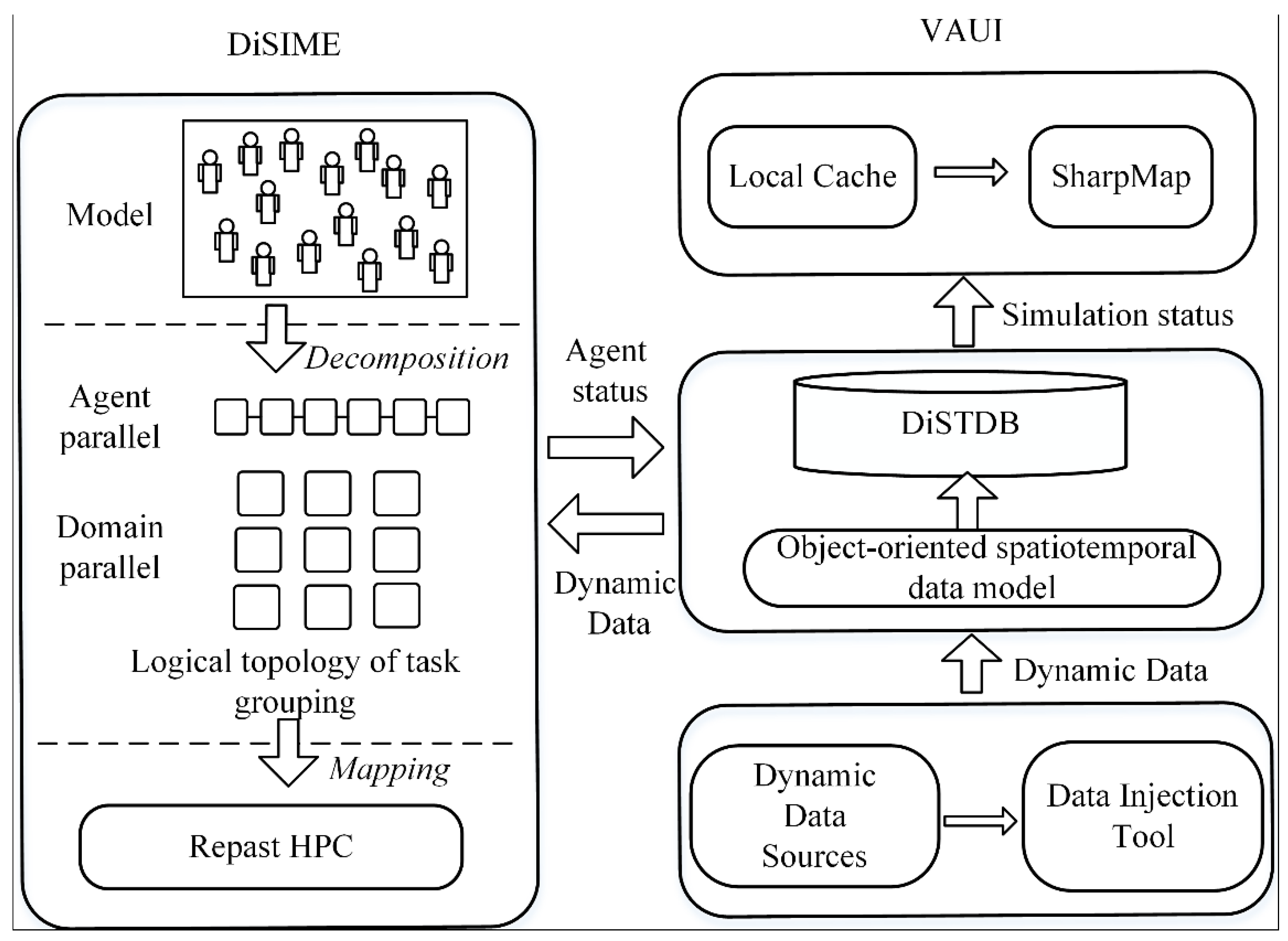
Figure 1. The proposed system is composed of three main components: distributed spatiotemporal database (DiSTDB), distributed ABM simulation engine (DiSIME), and visualization and online analysis UI (VAUI).
As shown in
Figure 1, the distributed spatiotemporal database (DiSTDB) is deployed as a storage center for the dynamic input data and the exchange center for the intermediate simulation results. This DiSTDB is built on a distributed MongoDB and supports fast query and updates. Dynamic data (e.g., road condition, wind direction) are collected and ingested into the DiSTDB by an additional data injection tool (DIT). These dynamic data are loaded by the simulation engine into simulation models; it will update the agent context status along with the model execution. The intermediate simulation results are continuously generated along the simulation, e.g., mobile agent’s positions, development of urban blocks. These intermediate simulation results can be also temporarily stored in the DiSTDB and later used for the scene update in the VAUI.
The distributed ABM simulation engine (DiSIME) is built on the open source project, Repast HPC (Repast for High Performance Computing), which can communicate with the underlying DiSTDB and supports the rapid development of geospatial simulation models. We carried out two main customization efforts on the Repast HPC. Firstly, the Repast HPC was extended to develop spatially-explicit ABMs. Several spatially-enabled classes are inherited from the original classes in the Repast HPC package. For example, the Agent class in Repast HPC can now include its own geometry that follows the OpenGIS Simple Features for SQL standard. The GDAL and GEOS libraries are used for importing/exporting spatial data into/from spatially-enabled agents. Secondly, the DiSIME can support different types of parallelism. In addition to the built-in “domain parallel” method, we developed an additional “agent parallel” method to support highly-mobile traffic simulations.
The VAUI leverages the power of traditional GIS visualization functionalities to support online representation of dynamic geospatial simulation. It can run on a stand-alone machine as a stand-alone executable program. It communicates with the remote DiSTDB through the query interfaces; this mode can separate the model visualization from the distributed simulation engine. At the same time, the VAUI provides an interface for clients to carry out visual analysis of geo-referenced time-series data.
4. The Distributed ABM Simulation Engine (DiSIME)
The distinct characteristics of DiSIME that differ from the original Repast HPC are the spatially-enabled classes (described in
Section 4.1) and the new “agent parallel” decomposition approach (described in
Section 4.2).
4.1. Reusable Components for GIS Phenomena Modeling
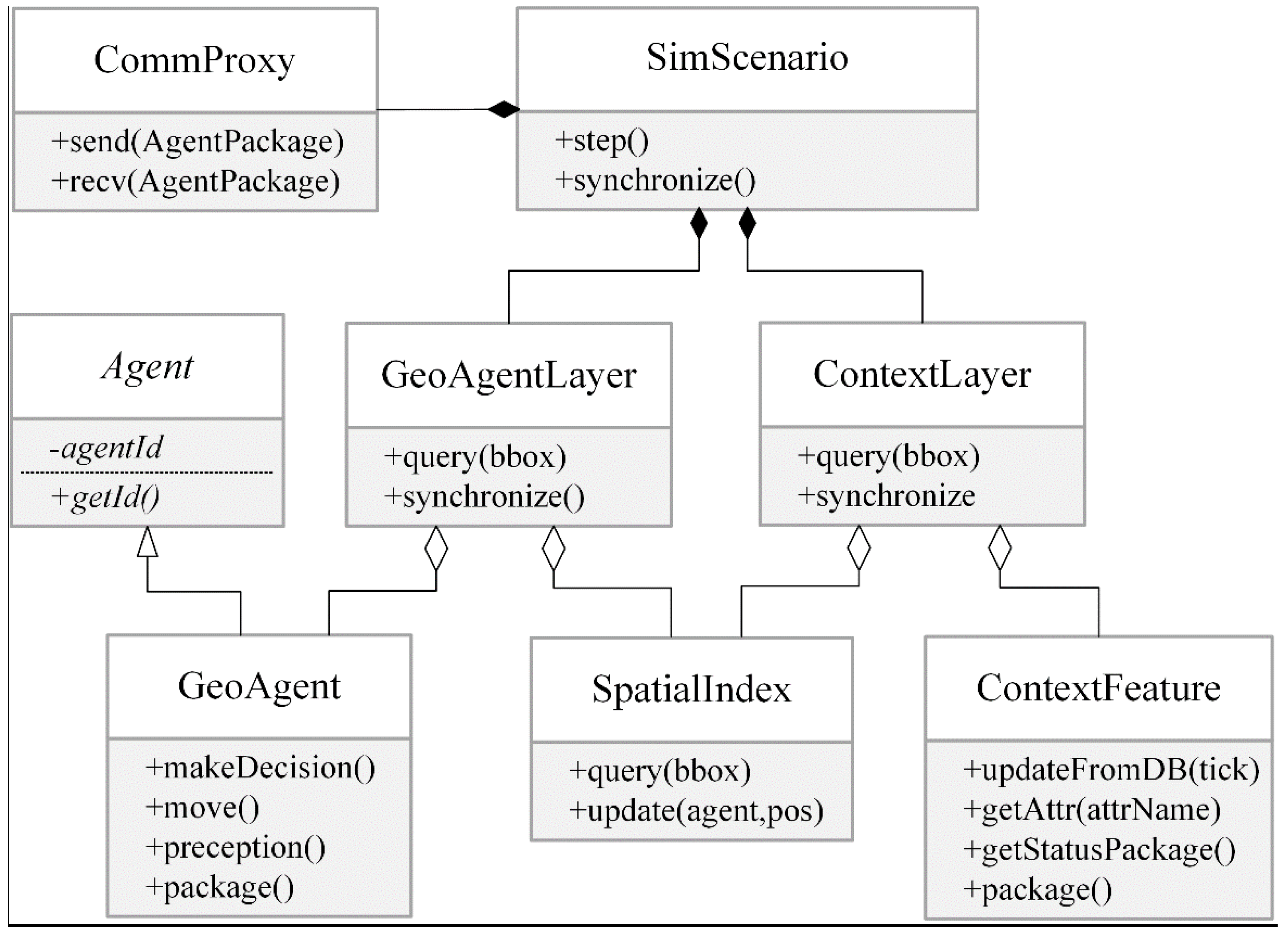
In order to support the rapid development of geospatial simulation models, several abstract classes were designed and integrated into the original Repast HPC package. All of these abstract classes have geospatial attributes and provide the ability to capture spatial phenomena. These classes make use of the power of C++ template types and are easy for reuse. The general relationship between these spatially-enabled classes is shown in
Figure 2.
The abstract classes, SimScenario, GeoAgentLayer, GeoAgent, ContextLayer, and ContextFeature form the kernel of a spatial agent-based model. The SimScenario class resides on the top level and manages all the components that define a simulation scenario. This class was implemented as a singleton object. It contains a set of GeoAgentLayer objects, a set of ContextLayer objects, and one CommProxy object.
The GeoAgent class extents the general Agent class in Repast HPC to represent all the dynamic spatial entities in the model that have internal states and make independent decisions. Here, the GeoAgent class is still a generic class containing abstract functions that need to be instantiated. Therefore, in an actual agent-based model, the developer should define a new domain-specific agent class, which is inherited from the generic GeoAgent class and provides concrete implementations for those abstract functions.
The GeoAgentLayer class acts as a container for a collection of spatial agents and defines the relationship between GeoAgents. Additionally, it also defines the aggregate representation of a group of spatial agents, e.g., in a grid or in a discrete team, and builds an agent topology and spatial index in this container.
The ContextFeature class represents the spatial features in the background context for agents. These spatial features in the context can be static or dynamic, and in a raster or vector format. The ContextLayer class has the same function as the GeoAgentLayer class and acts as a container for the ContextFeature objects.
The SpatialIndex class implements common spatial indexes as R-Tree, grid-based index, and KD Tree to accelerate spatial queries. The original Repast HPC platform only supports agent query by ID or exact position. This SpatialIndex class complements the agent query types in Repast HPC. The CommProxy (short for “Communication Proxy”) class is responsible for agent interaction and state synchronization between the distributed simulation nodes. For example, it can help exchange the status of some agents which reside in two adjacent nodes to make them consistent.
4.2. The “Agent Parallel” Decomposition in the DiSIME
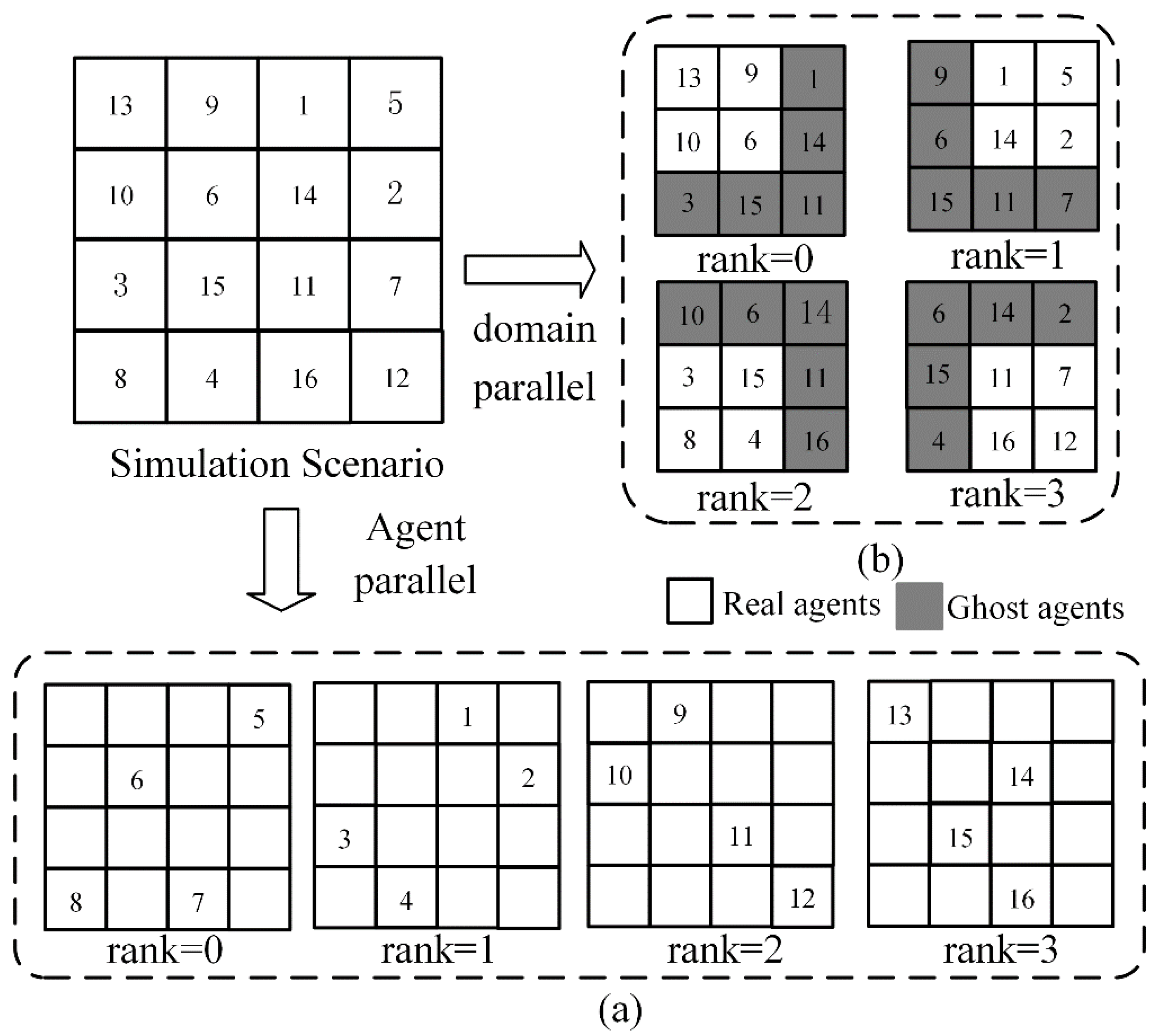
Extended from Repast HPC, the parallel agent modeling in the DiSIME now can exploit two types of parallelism: “agent parallel” and “domain parallel”, illustrated in the
Figure 3. Repast HPC provides an intrinsic spatial decomposition for the distributed ABM simulation,
i.e., “domain parallel”. The “domain parallel” approach divides the geographic space into discrete sub-divisions and each sub-division contains a partial portion of all agents that reside in this region. Thus, the sub-divisions in the domain decomposition can be directly mapped to MPI processes.
However, the domain parallelism seen in
Figure 3b does not fit well in the highly-mobile traffic simulation. Cars travel back and forth in the complex road network. If the “domain parallel” decomposition method is adopted for this case, car agents move frequently from one sub-division to another sub-division, these shuffles will cause high communication between processes and result in severe load imbalance. Due to this problem, Repast HPC has been extended in the DiSIME to support another decomposition method, “agent parallel”, seen in
Figure 3a. In this parallelism all the agents are decomposed only with consideration of agent orders and without reference to any spatial structure of agents and their context. For example, a total of 1000 mobile cars in one traffic model might be divided into ten groups: 0~99, 100~199, …, and 900~999. This type of parallelism is suitable for the cases where there is little commutation among agents but more communication between agents and their context.
In the Repast HPC, the Projection class is used to define the agent context and impose a semantic relationship on agents. It provides three projections: a network, a grid and a continuous space. All of them are split and distributed over the MPI processes during the simulation. However, none of these three projections are suitable for the “agent parallel” case. In order to implement “agent parallel” decomposition, the ContextLayer class is directly extended from the generic Projection class. In this new projection, all the context data are duplicated among the simulation processes. The master process is responsible for updating all context copies and makes them consistent during the whole model execution.
In the “agent parallel” decomposition, the communication between processes is mainly composed of general statistics of spatial agents, e.g., total number agents in a specified region. In order to support this kind of GIS operations, the CommProxy class extends the RepastProcess class to support spatial queries across processes. The agent request message contains only a spatial range to request those GeoAgents who falls within this region without providing exact agent IDs. During message communication, the GeoAgent’s geometry data is firstly encoded into a WKB (well-known binary) string with the help of GDAL library and then transmitted together with thematic attributes to the destination process by MPI. At the destination process, the WKB string is then decoded by CommProxy into a Geometry class to carry out spatial queries.
5. The Management and Injection of Dynamic Spatial Data
To implement the required functions of the DiSTDB, a spatiotemporal data model was designed to efficiently represent all the dynamic information for ABM simulation and visualization. This data model is described in
Section 5.1. The additional data injection tool (DIT) is introduced in
Section 5.2 to show how to collect and assimilate dynamic data into the DiSTDB.
5.1. The Object-Oriented Spatiotemporal Data Model
Many GIS data models have been proposed to incorporate temporal information into spatial databases, including Sequential Snapshots [
43], Base State with Amendments [
44], Space-time Composite Model [
45], Object-oriented Spatiotemporal Model [
46], the Event-based Spatiotemporal Data model [
47],
etc. Several studies have made detailed survey about those spatiotemporal data models [
43,
48]. In order to effectively incorporate and store dynamic data from different sources, the data model in the DiSTDB is extended from the simple snapshot data model and the object-based spatiotemporal model.
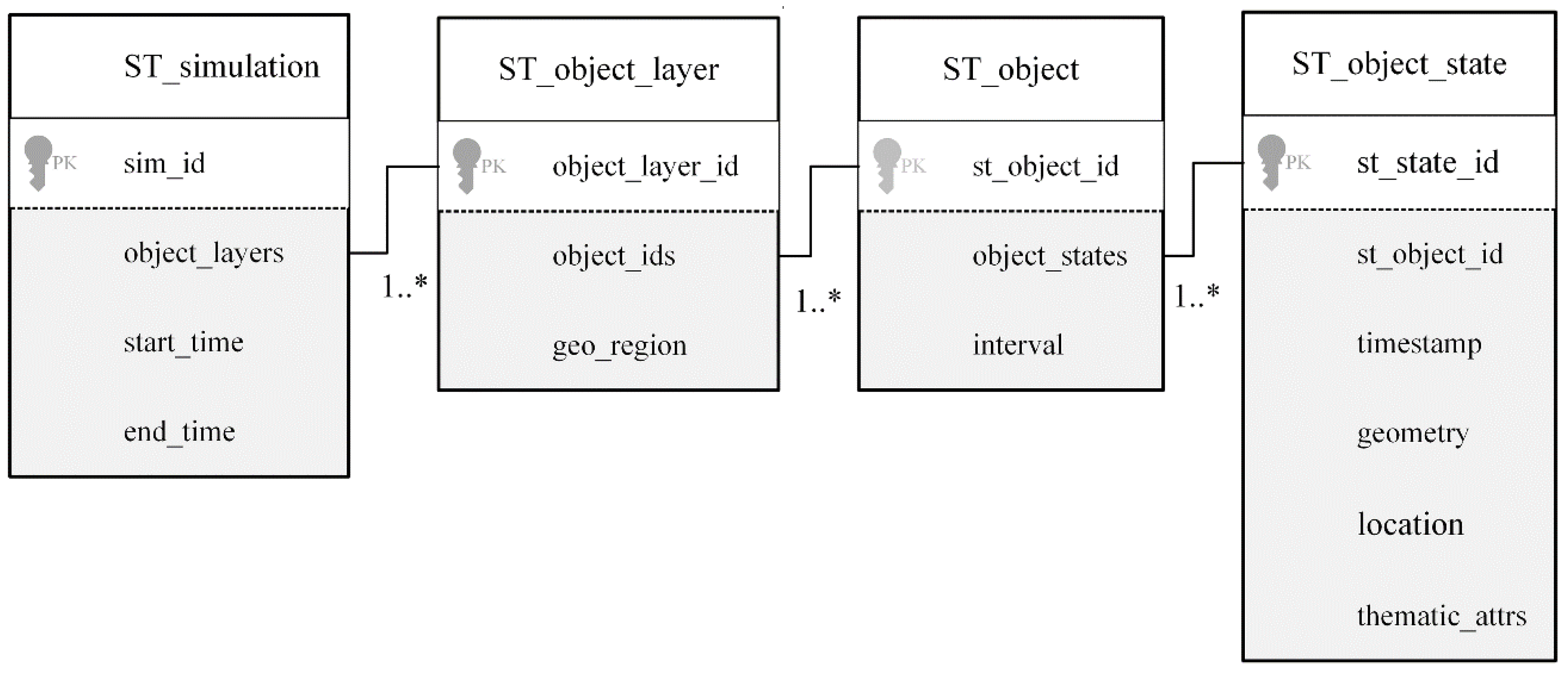
Figure 4 depicts the entity–relation (ER) diagram of the proposed spatiotemporal data model. This data model is comprised of several primary building blocks, ST_simulation, ST_object_layer, ST_object, and ST_object_state, respectively. A ST_simulation represents one simulation process in the DiSIME and contains a set of spatial object classes, called the ST_object_layer. Every ST_object_layer is a collection of temporally-homogeneous spatial objects (
i.e., ST_object), and each object has a number of temporal states (
i.e., ST_object_state), which are associated by a time tag. In each temporal state, each object has one geometry and a number of thematic attributes. A state of the spatial object might be a change in the geometry, attributes, or both. This customized snapshot model might cause a degree of data duplication with unchanged properties in space or time, but this tradeoff will become very efficient when faced with concurrent status updates from different sources. The entities in this spatiotemporal data model have a direct relationship with the abstract classes in the DiSIME. For example, the GeoAgentLayer and ContextLayer from DiSIME can be serialized into the ST_object_layer table in the DiSTDB, while the GeoAgent and ContextFeature are both stored in the ST_object table.
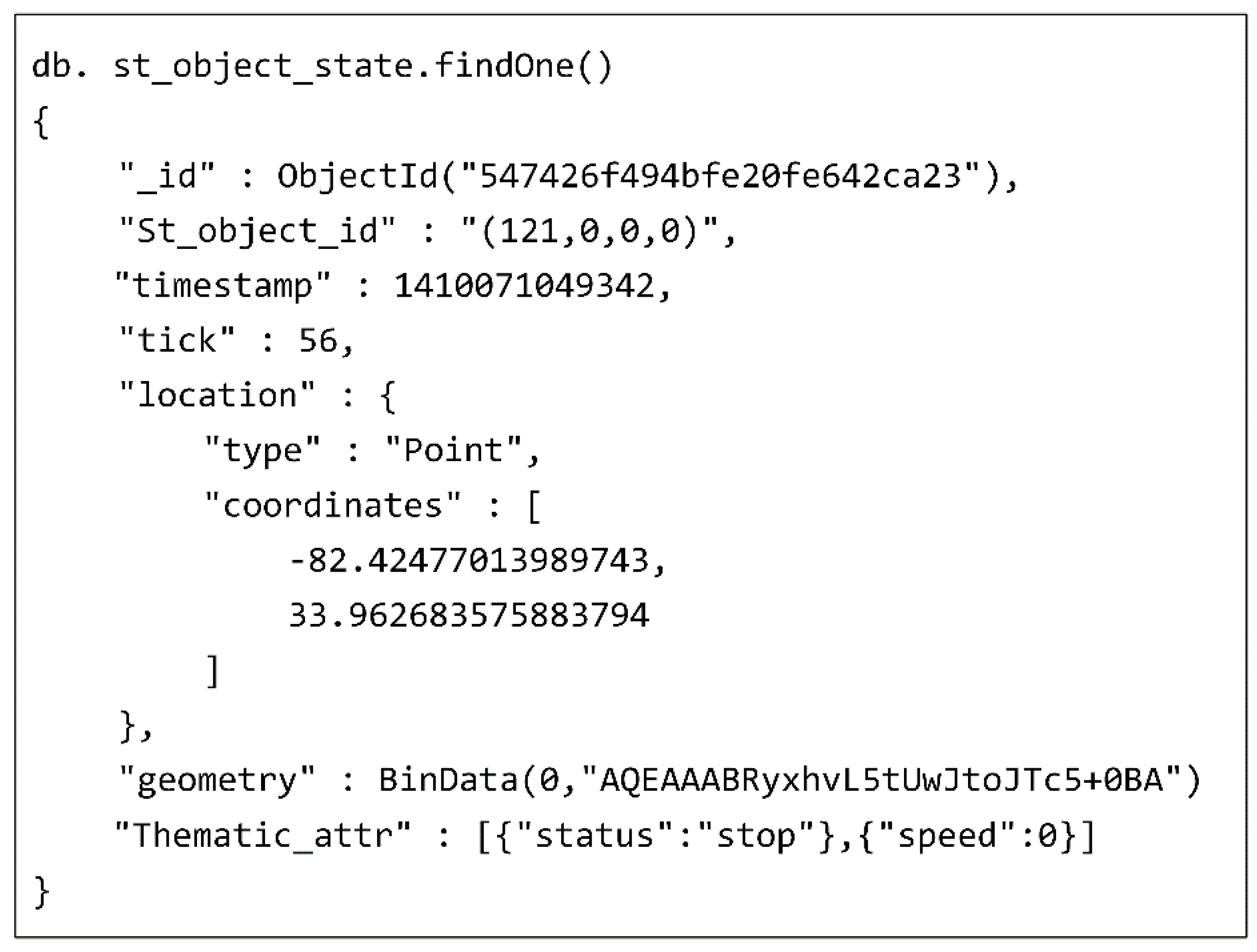
The MongoDB is chosen to implement this above-mentioned spatiotemporal data model. Here one state record from the ST_object_state table is selected to illustrate how the dynamic spatiotemporal data is stored in the MongoDB JSON format, a record example is shown in
Figure 5.
5.2. The Concurrent Data Injection Pipelines for the DiSTDB
During the dynamic-data driven simulation, both the agents and context in the ABM, i.e., the ST_object_state tables in the DiSTDB, are frequently updated along the simulation. The two update processes are different between them. The status of spatial features residing in the background context is updated from the observation data by the Data Injection Tool (DIT), while the status of different agent objects is updated by the temporary simulation results directly from the DiSIME.
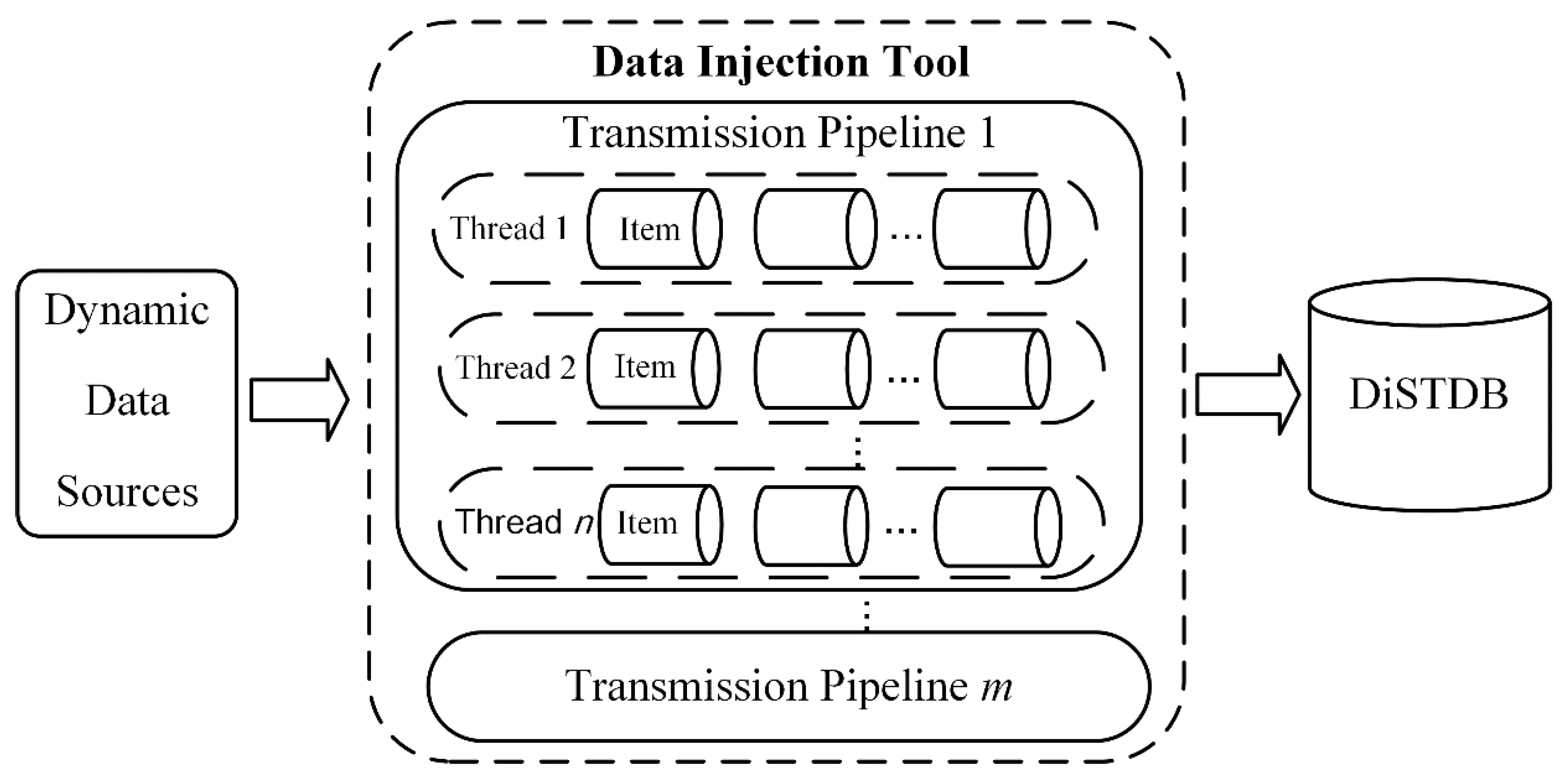
The data injection tool internally spawns a number of data stream pipelines, shown in
Figure 6. One side of the stream pipeline is the sensor data provision interface, e.g., OGC SOS (sensor observation service), and the other side is the predefined table in the DiSTDB. The pipeline periodically reads the observation data from the provision interface processes the input data with selected filters and appends a new object state record to the specific spatial object in the target DiSTDB.
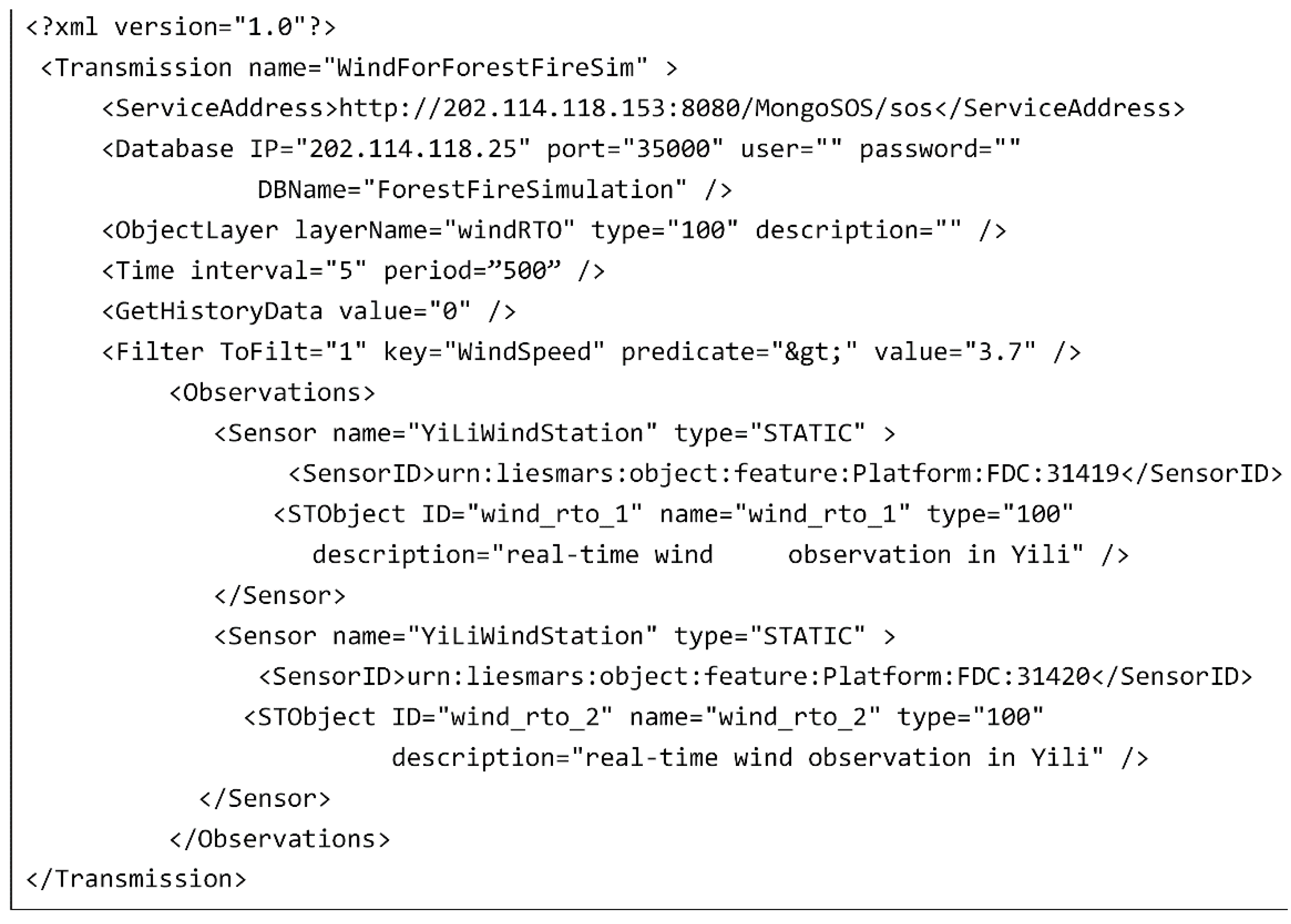
Each stream pipeline usually has n concurrent working threads and these working threads execute the transmission tasks. In the streaming DIT pipeline, each observation data is encapsulated into a Transmission Item which acts as the transmission payload. The Transmission Item is formatted with a XML file and defines the source, destination, and the attached filter operations. One XML Transmission Item sample for wind speed data is illustrated as follows in
Figure 7.
6. Dynamic Visualization of ABM Simulation
The VAUI in the 4D-SAS is responsible for dynamic visualization and online analysis. The VAUI uses the open-source SharpMap as the visualization environment, and takes advantage of its functionalities to render a realistic display. SharpMap, written in C#, is an easy-to-use GIS mapping library for use in web or desktop applications. SharpMap was developed originally for static map visualization, and so must be adapted to the needs of dynamic simulation modeling. The VAUI extends traditional GIS functionalities of SharpMap with three new features: (1) direct communication with the underlying DiSTDB; (2) interactive display of dynamic simulation process in animation; and (3) online analysis of geo-referenced time-series data.
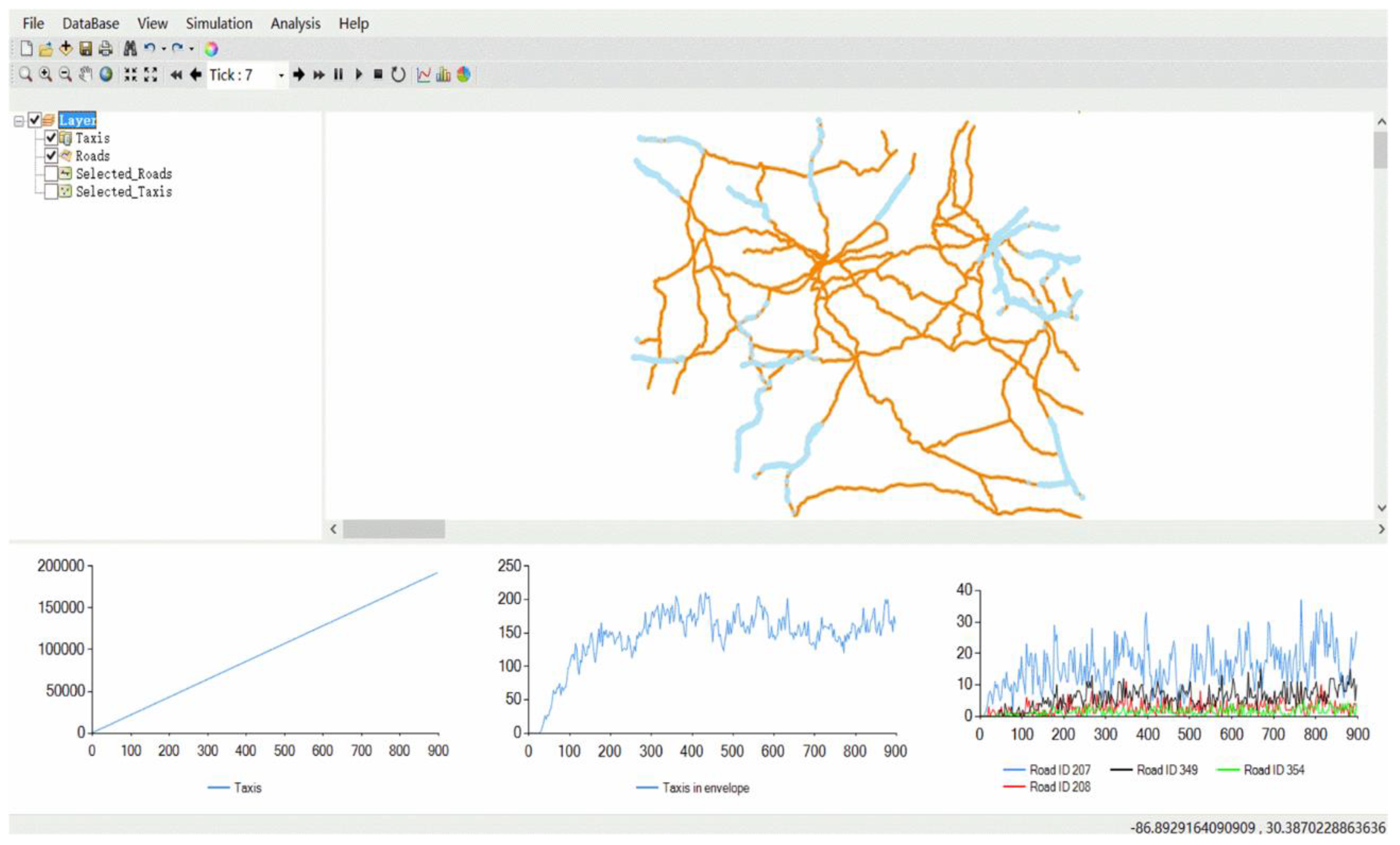
The simulation visualization is time-aware and presented with user-controlled animations. The VAUI periodically extracts dynamic simulation results from the DiSTDB and dynamically updates the simulation scene at a given frequency, illustrated in
Figure 8. Besides the basic GIS view functions, e.g., zoom in/out and pan, it also provides the capability to make snapshots of the display and movies of the model development as it evolves over time. It allows users to control a running simulation (
i.e., start/stop the simulation, adjust parameters, save/load simulation states) through the control panel. Furthermore, the VAUI allows users to query detailed properties of simulation entities (e.g., current vehicle speed) through query tools. It also includes convenient tools for real-time calculation of statistical values in the temporal dimension, for example, median values over a selected time period.
7. Case Study and Experiments
7.1. Experimental Design and Configuration
Two simulation cases were developed to evaluate the efficiency and suitability of the proposed 4D-SAS. The first case contains thousands of mobile agents and demonstrates the development of an “agent parallel” model, while the second case uses a cellular automata-based ABM to evaluate “domain parallel” model development. During the two experiments, two metrics, speedup and parallel efficiency, were employed to evaluate the performance of these two parallelized models.
All of the experiments were conducted on a cluster of high performance computers. The cluster consisted of 13 machines configured as follows: one machine was used as the cluster manager; one machine was used as the VAUI visualization; six servers were used as the computing units of the DiSIME, and five servers were for the underlying DiSTDB. All of the servers were directly connected by a dedicated 1 Gbps Ethernet. The detailed configuration of the cluster is listed in
Table 1.
7.2. “Agent Parallel” Model Simulation Case Study
This first experiment used an en-route driver choice model to show how an “agent parallel” model can be built and run on this system. The model in this case simulated route switching by individual drivers on the highway when provided with real-time traffic information.
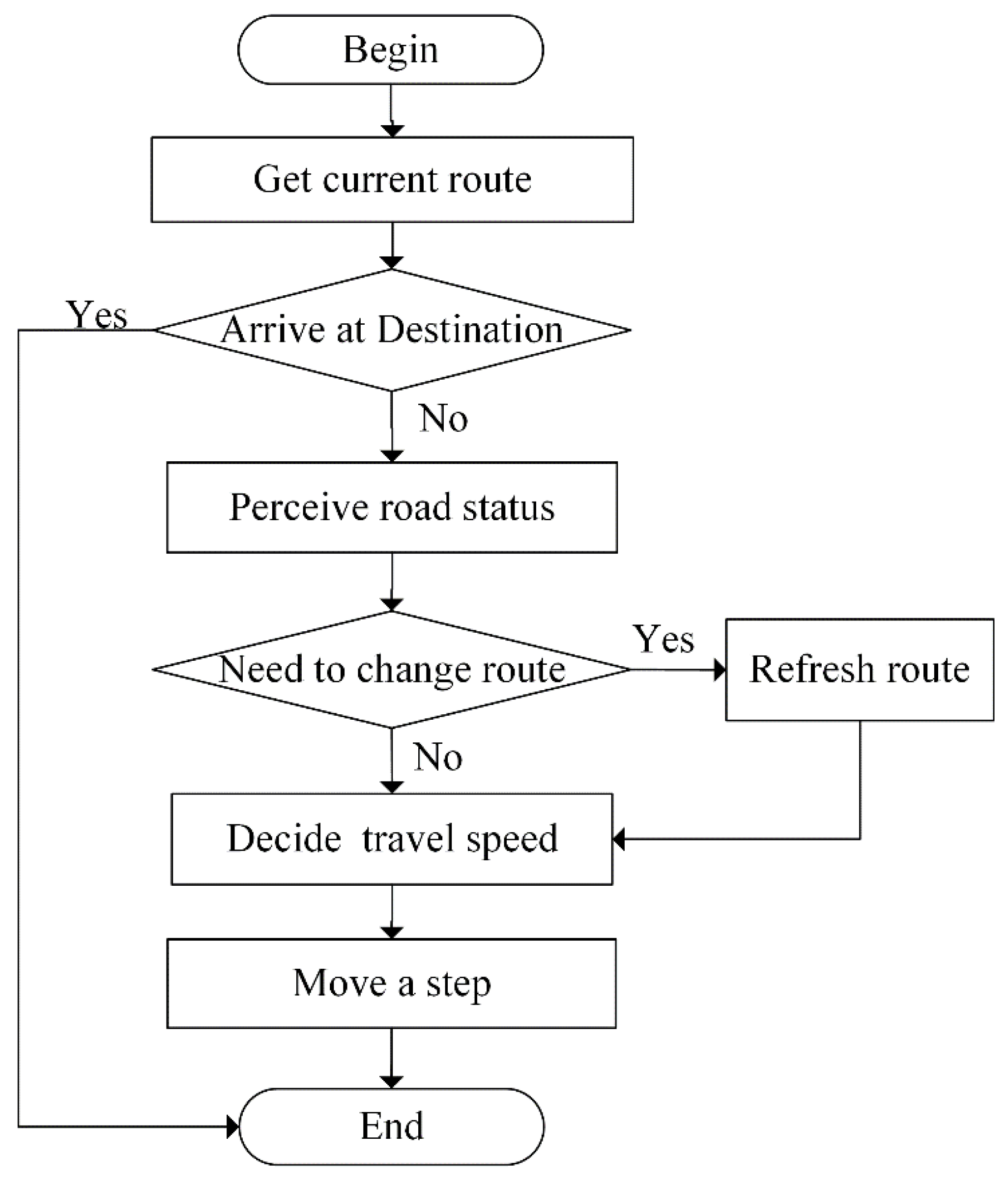
Figure 9 is the flow chart of the designed en-route driver choice model.
This en-route driver choice model is tested with 10,000 mobile car agents and a road network dataset of the contiguous United States. The road network is composed of 86,141 edges and 68,909 nodes. Shown from
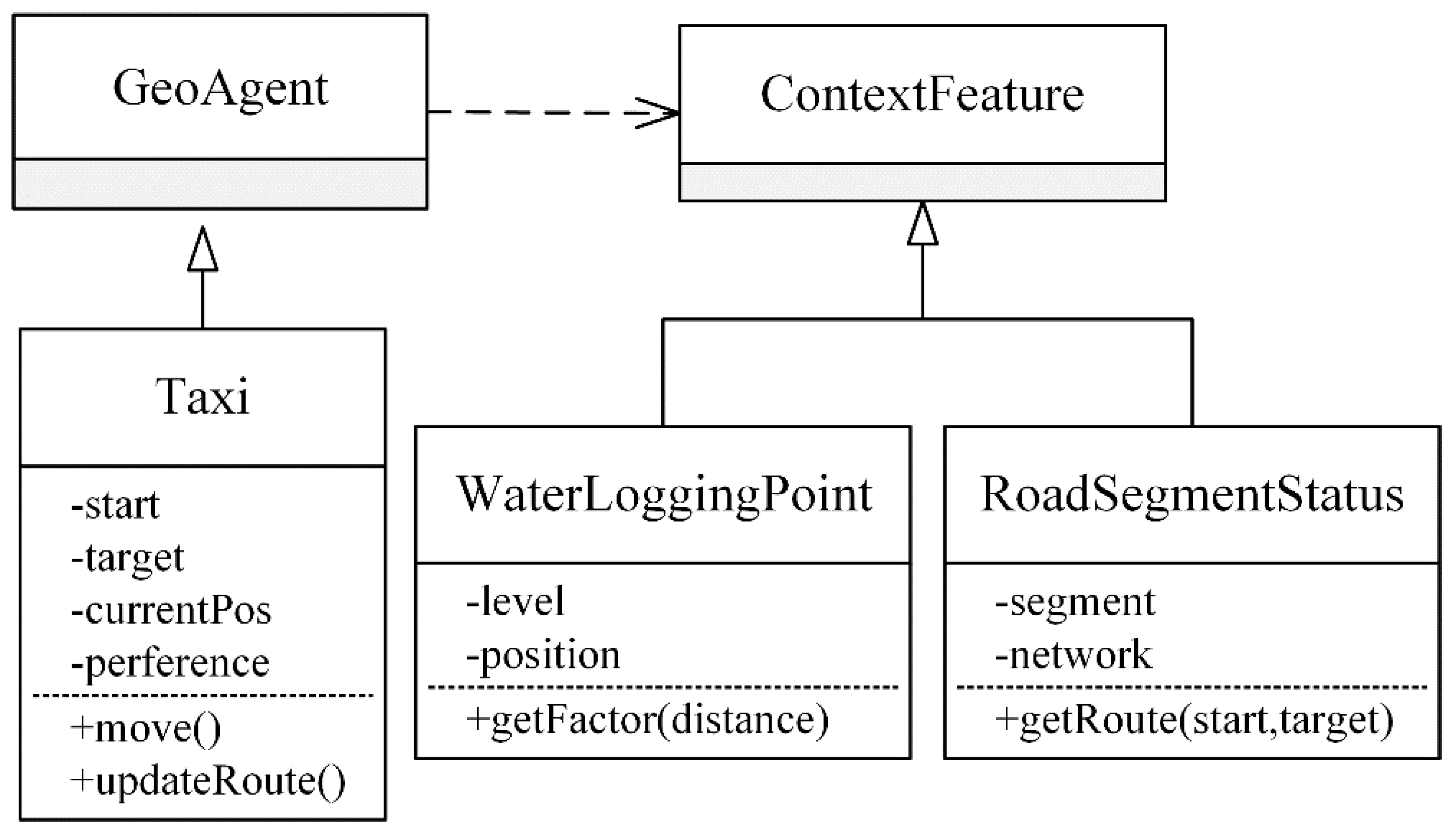
Figure 9, the origin and destination of each car agent was randomly selected before the simulation. In this simulation, a random transportation emergency, such as water-logging, has taken place in the road network and blocked the transportation around it. The real-time information, e.g., the status of the road network, was collected and broadcasted to all the mobile car agents. When fed with the real-time traffic information, the mobile car agent makes a decision and selects an alternative route according to the least travel cost (
i.e., travel time here). Based on the abstract classes in the DiSIME, a Taxi agent class inherits the decision-making role from the GeoAgent class in the model, and two additional ContextFeature classes, WaterLoggingPoint and RoadSegment, are derived as the dynamic context, illustrated in
Figure 10.
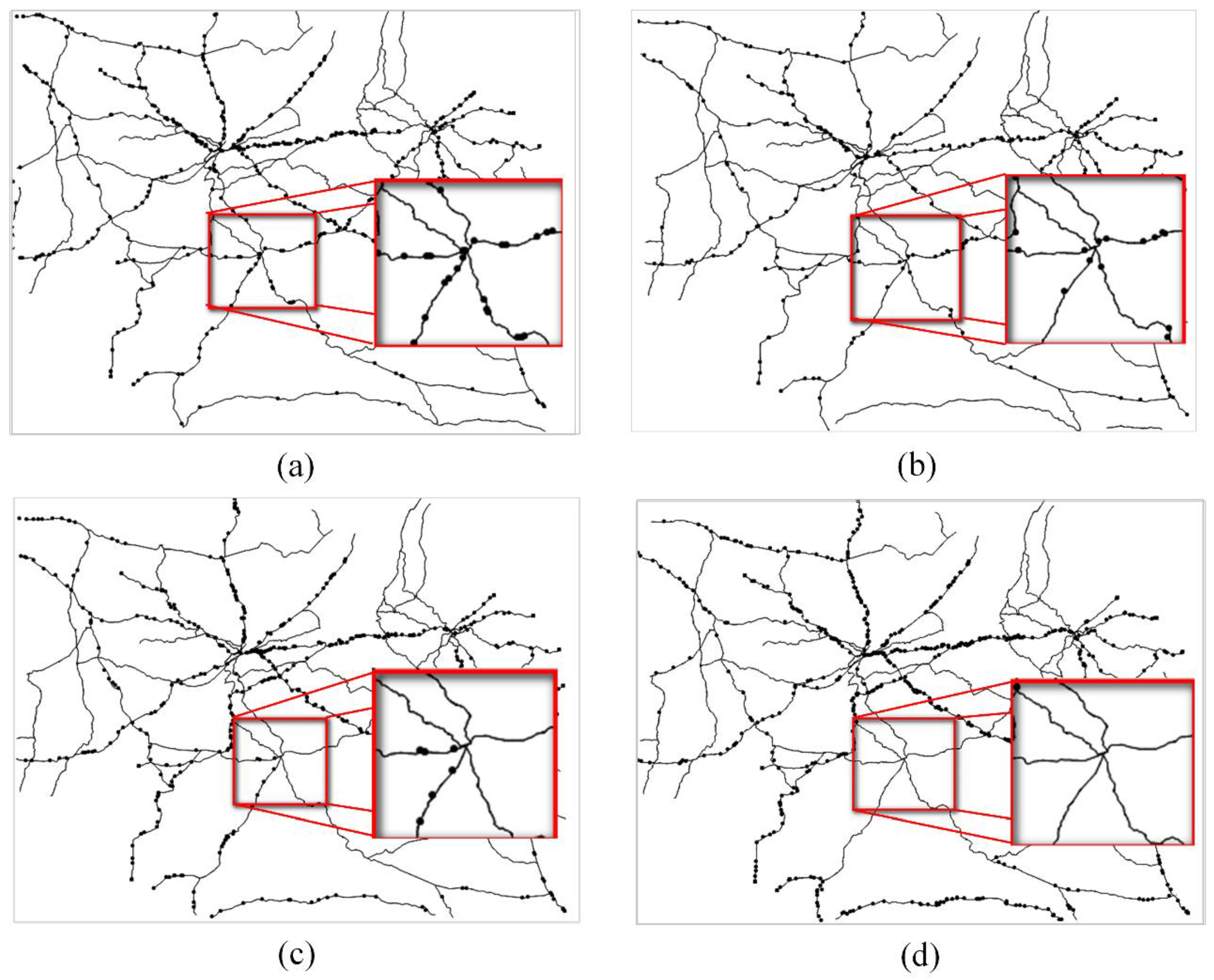
Figure 11 shows the dynamic simulation process of the en-route driver choice model. There is a waterlogging occurring in the red rectangle area (
Figure 11a). As the waterlogging becomes heavier (the water level in
Figure 11b–d changes from 1 to 3), fewer taxies will go through this area, causing a heavy transportation load on other roads.
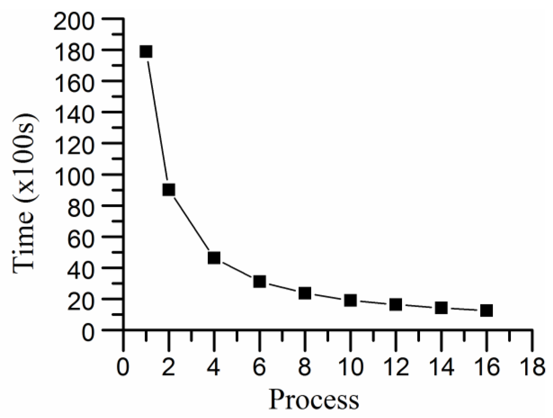
The whole mobile cars are split following their order and distributed to different computing units. The total simulation time is measured with different execution node configurations, as shown in
Table 2. Shown in
Figure 12, as the number of simulation node increases, the total model execution time decreases sharply.
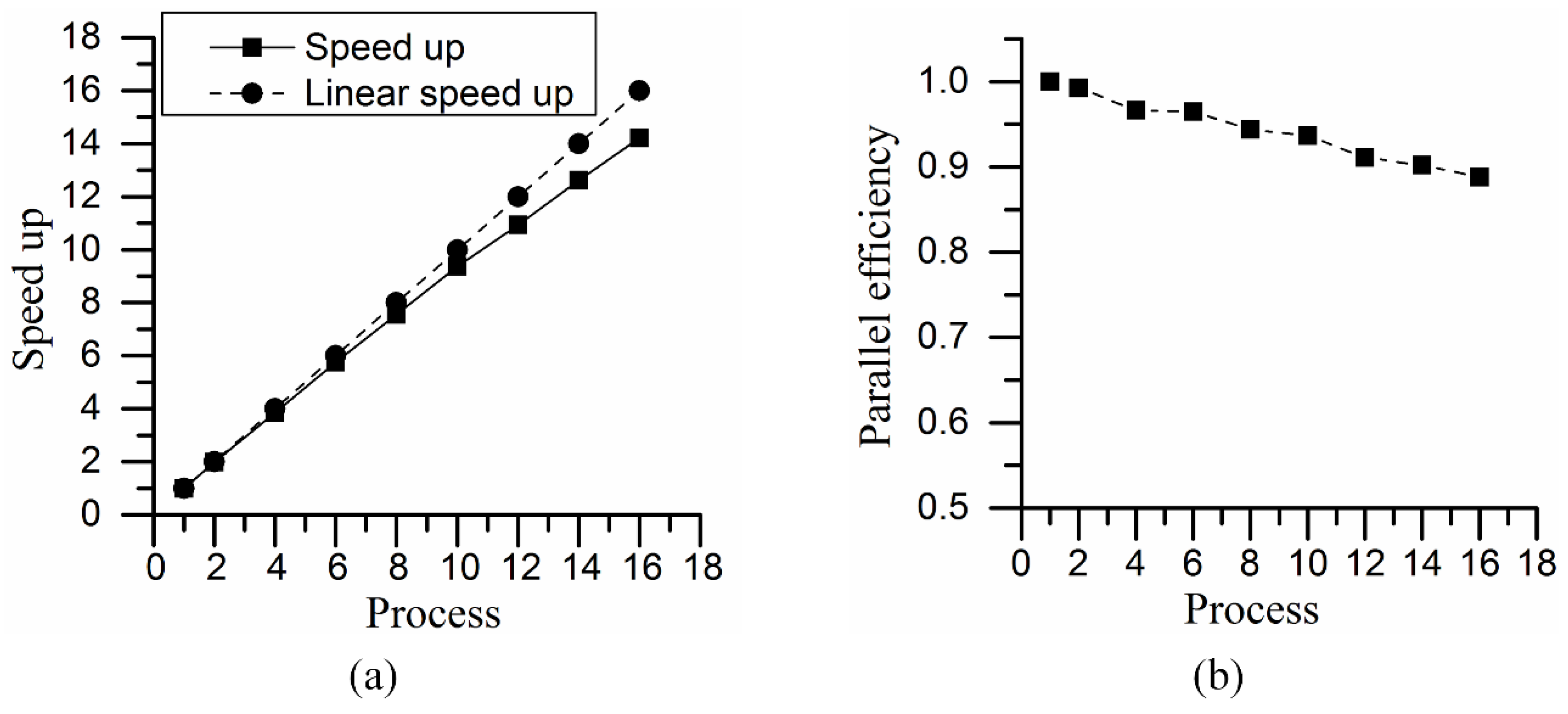
As shown in
Figure 13, the total speedup is nearly linear because there is no communication between the mobile agents. However, when the processor number increases to eight, the total execution time decreases more slowly and the parallel efficiency drops from 1 to about 0.88. Generally, the implementation of this parallel en-route driver choice model on the 4D-SAS system is trivial, but its scalability is very high, consistently around 90%.
7.3. “Domain Parallel” Model Simulation Case Study
This second case can examine how this system can support the development of a “domain parallel” model. This experiment uses a cellular automata (CA) model to describe the dynamics of forest fire spread on a mountainous landscape.
CA-based model has been a mature approach to model the spread of forest wildfires [
22,
23,
24,
49]. In the CA-based models, the geographic landscape is firstly divided into a 2D array of identical square units and each unit is represented by a cell agent in the model. The fundamental factors of a CA model include the initial state of a cell and the state update rules (e.g., unburned, burning, or burned) from one temporal interval to the next. By this way, the model can calculate the arrival time of fire front from one cell to the next. The local update rules usually depend on the property of this cell and the states of its neighbor cells.
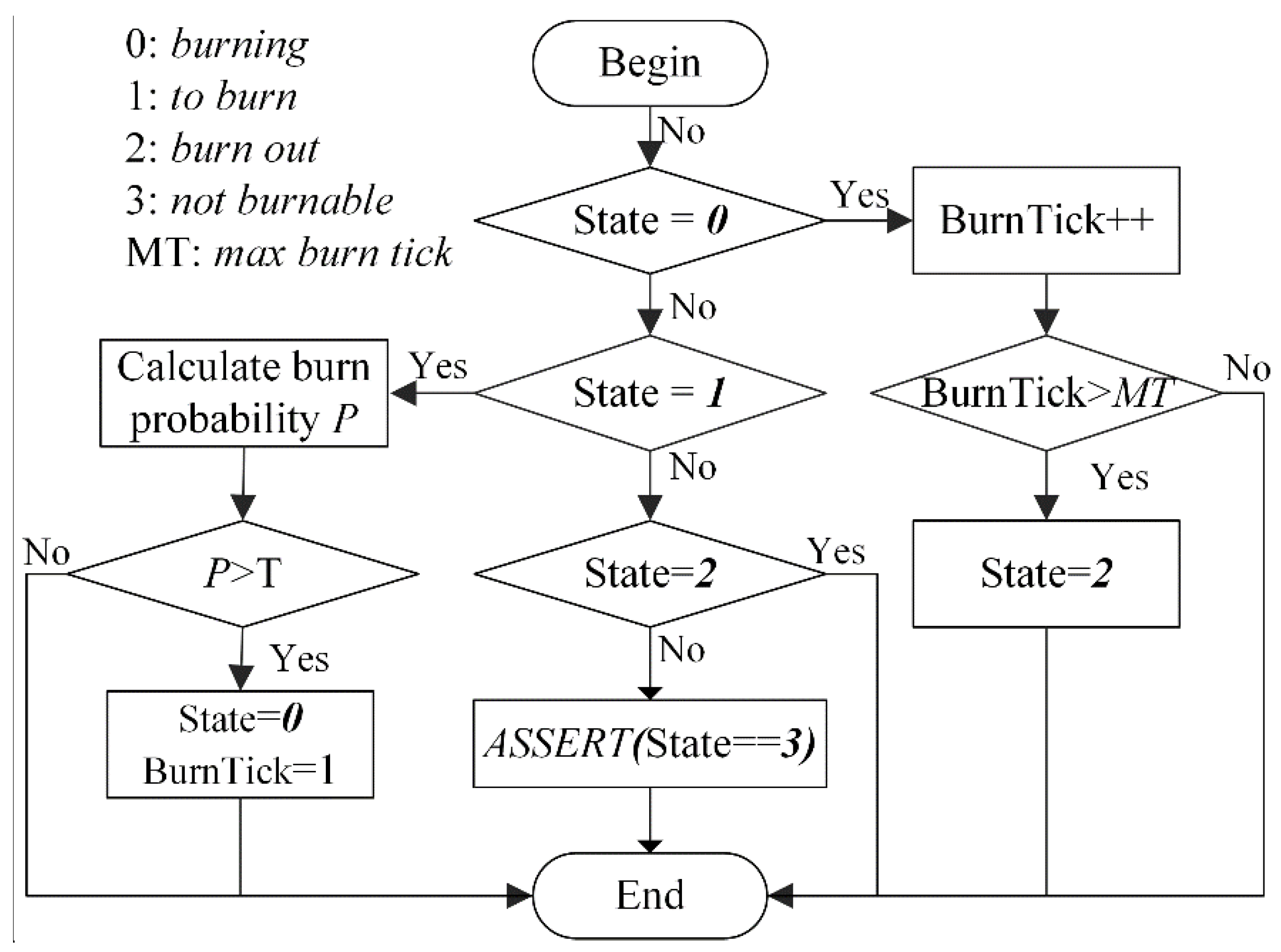
Figure 14 is the flow chart and state update rules of the designed CA-based forest fire spread model.
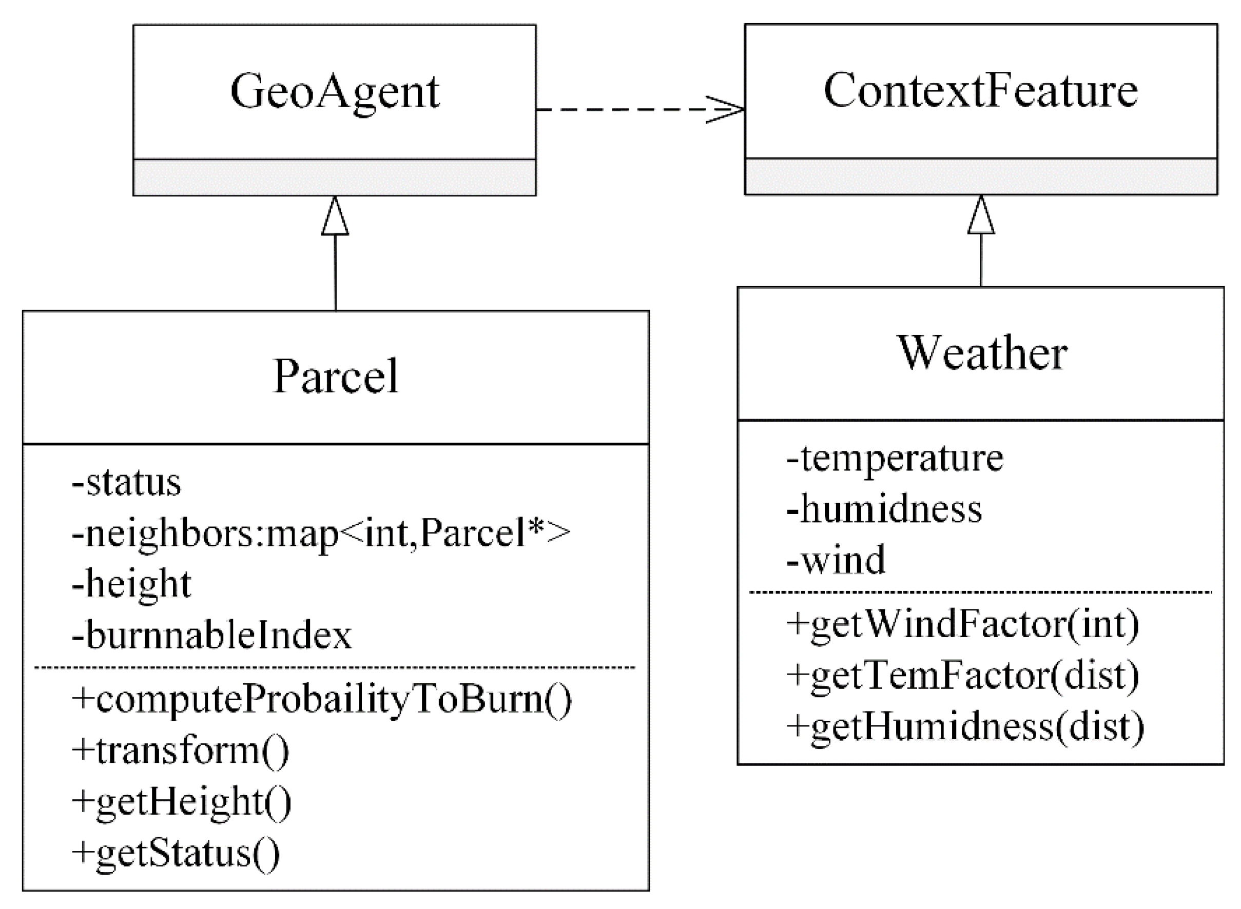
The real-time weather information is collected in advance and fed into the forest fire simulation model, including wind speed, wind direction, temperature, and humidity. Wind speed and its direction forms a vector parameter. The environment temperature is a scalar parameter. The higher the temperature is, the greater probability that the land cell with burning neighbors will burn. The environment humidity has a value range from 0 to 1. The higher humidity will result in less probability for the land cell to burn. Vegetation density, vegetation type, and terrain slope information are extracted from remote sensing imagery and digital elevation models. As in the first case study, two new classes, Parcel and Weather, are derived from the abstract DiSIME classes, as illustrated in
Figure 15.
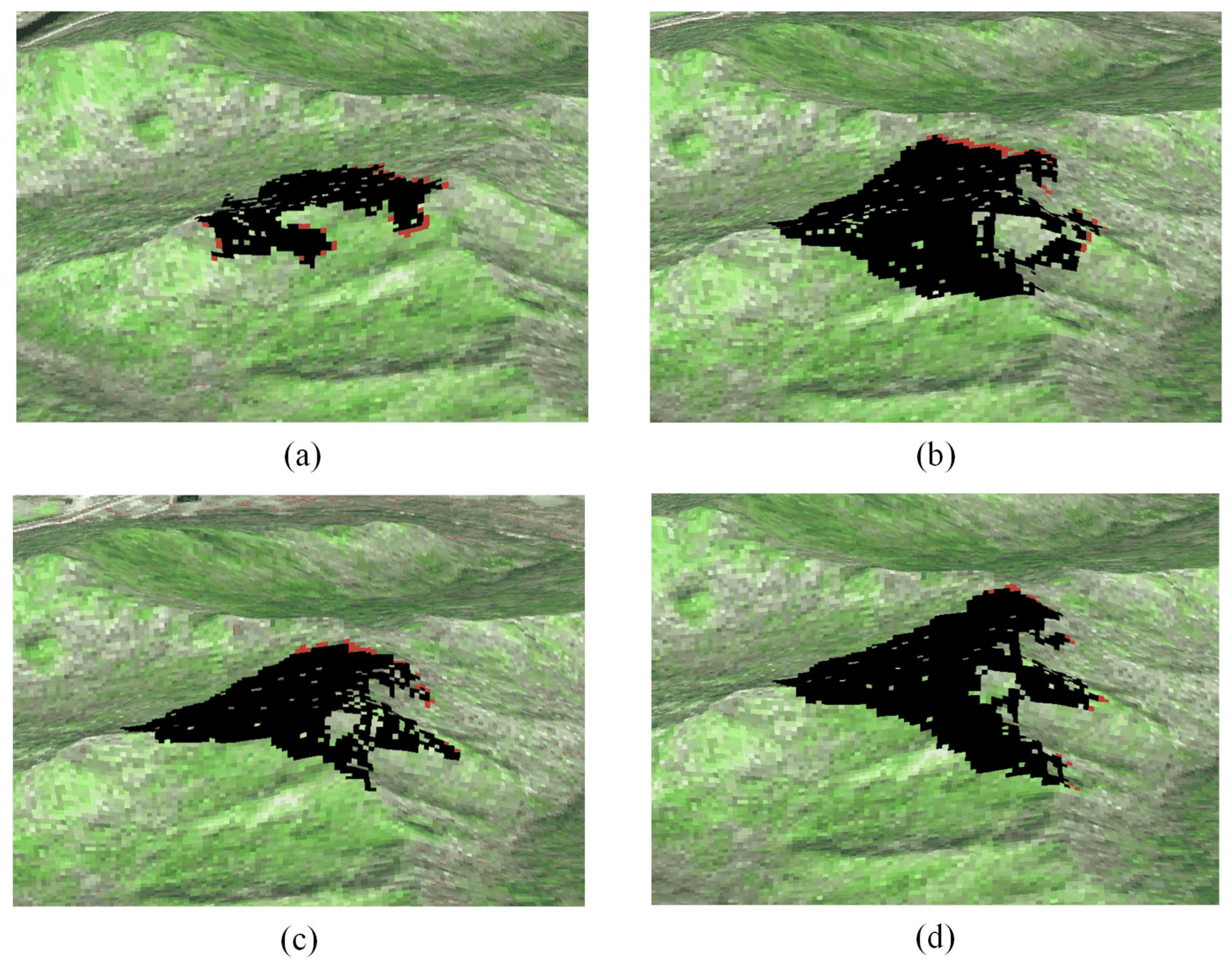
The 2D CA grid size is 7721 × 6233 pixels with pixel resolution of 30 m. The simulation results of the fire spread are shown in
Figure 16. The black color parts are the final burned area while the red lines show the evolution of the fire front at 1h interval. The four pictures illustrate the fire spread with a fixed wind direction but with different wind speeds: (a) is 0 km/h, (b) is 5 km/h, (c) is 10 km/h, and (d) is 15 km/h. Based on the “domain parallel” method, all the cells are divided into a collection of equal rectangles which will then be distributed to different computing units.
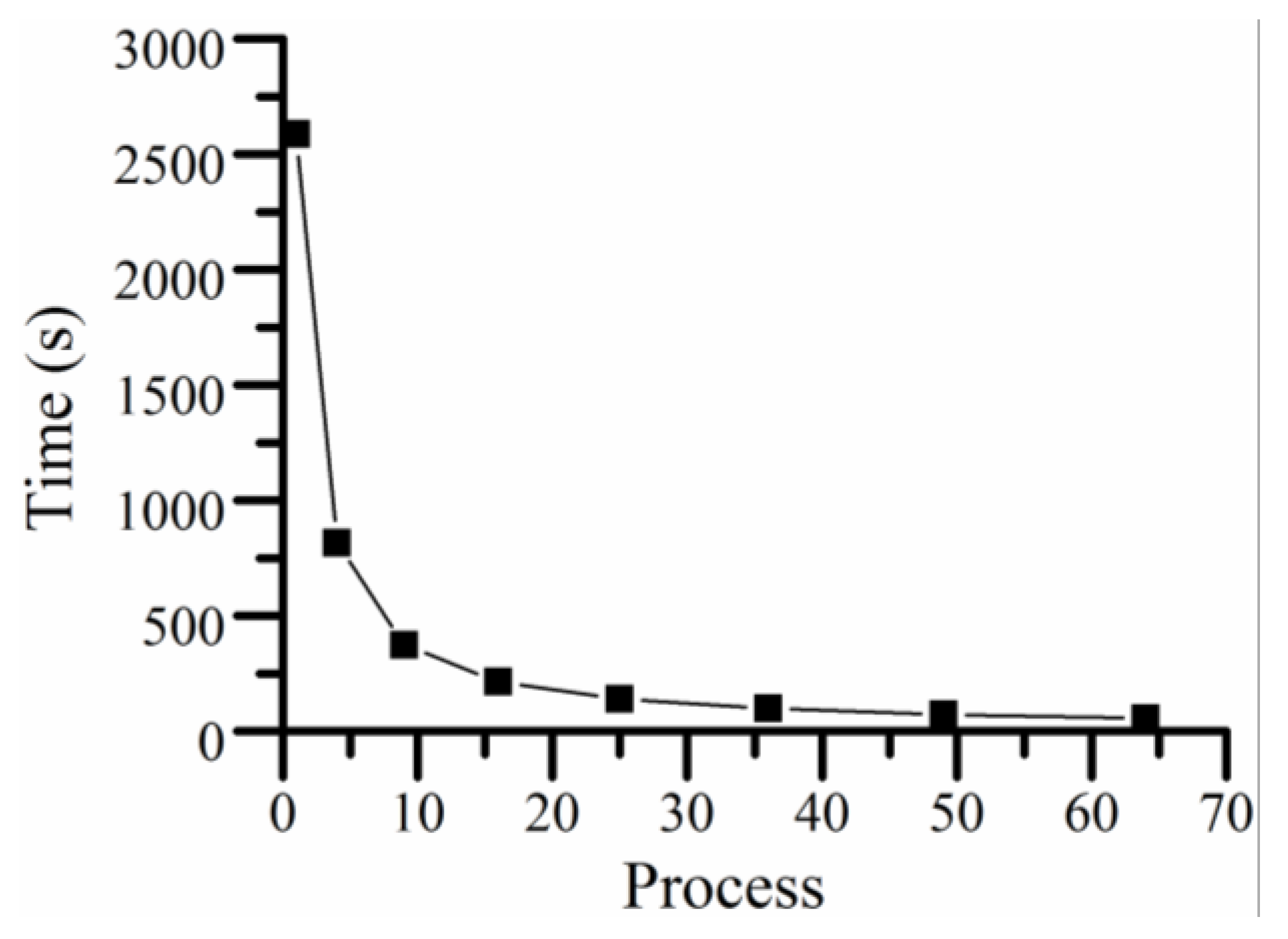
Table 3 lists the total simulation time with different execution node configurations. Shown from
Figure 17, when the number of simulation nodes increases from one to 16, the execution time decreases very quickly.
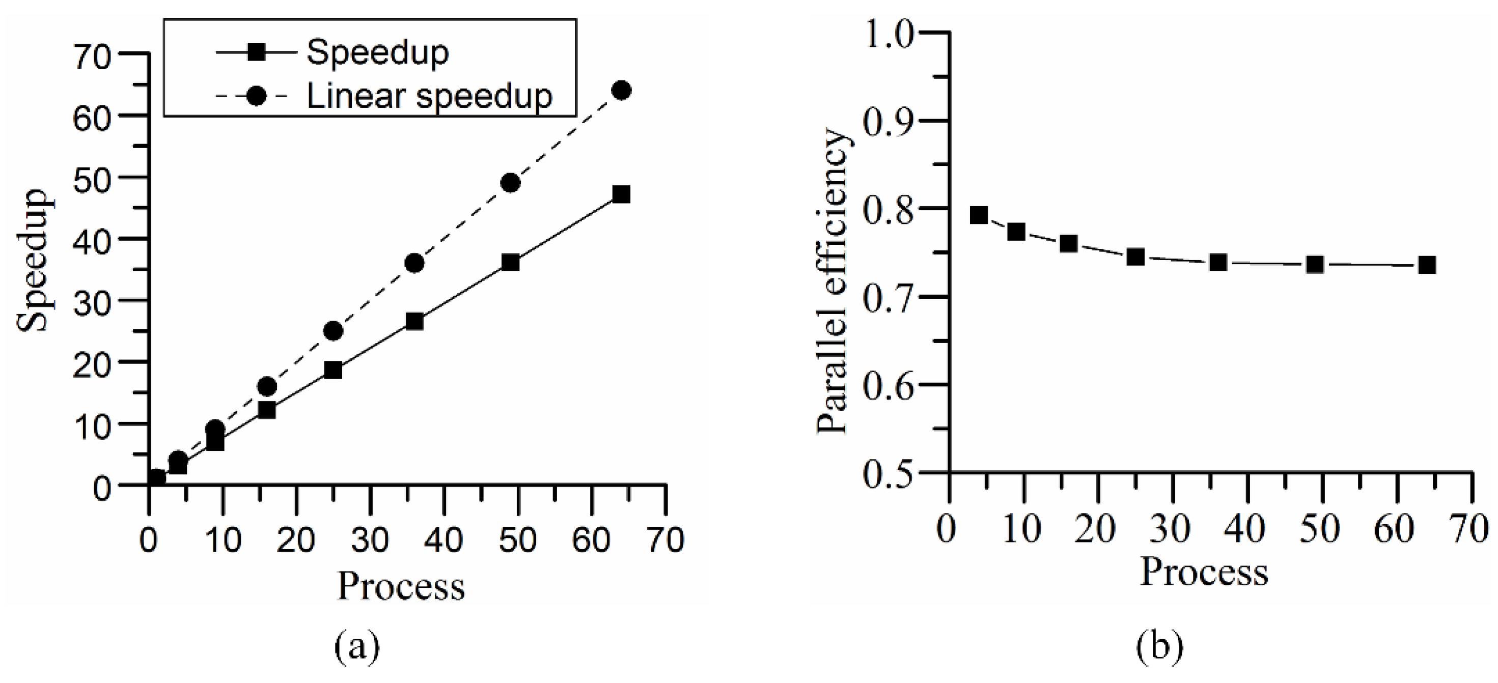
Figure 18 shows the corresponding speedup and parallel efficiency.
When the number of simulation node increases over 16, the execution time decreases much slower. The total speedup increased steadily from nearly three to about 36, while the parallel efficiency was around 0.75 and did not change too much.
7.4. Discussion
During these experiments, two simulation models represent two typical simulation scenarios. The first model represents common multi-agent simulations, which contain a collection of discrete, intelligent, and frequently-moving agents. The second model represents common grid-based cellular automata simulations, in which the cells are fixed but have frequent status transitions. The development of these two models in the proposed 4D-SAS shows that the 4D-SAS can provide an efficient platform for dynamic data-driven geospatial modeling. Compared with existing parallel simulation platforms, including FLAME, DMASON, and Repast HPC, the 4D-SAS directly integrates spatial data into model-building, e.g., Shapefile-based road network in Case 1, remote-sensing imagery and DEM in Case 2. This spatial data integration capability of 4D-SAS greatly enhances model representation and decreases model building costs. These existing platforms always define all the model inputs before simulation. In contrast, the 4D-SAS successfully incorporates real-time dynamic data when executing simulations. This dynamic incorporation can provide up-to-date information for model context and obtain more accurate simulation results, which can provide support for decision and planning.
In these two parallel simulations, the two parallel efficiencies were both above 0.7. Illustrated in
Figure 13b and
Figure 18b, the parallel efficiency of the driver choice simulation is a little higher than that of the fire propagation simulation, about 0.9
vs. 0.75. This can be attributed to frequent agents’ status request and updates between the adjacent rectangles in the fire propagation simulation. During each iteration, each rectangle will request the current status of the overlapping cells from the neighboring rectangles and update the corresponding cells in its region. Conversely, the mobile agents in the driver choice simulation are independent and there is no direct communication between each other. During the driver choice simulation, the master node needs only to collect the coarse context status from all computing nodes to obtain the overall statistics and scatters this information to all the slave-computing nodes. The communication overhead in the driver choice simulation is much lower than the fire propagation simulation. Therefore, the parallel efficiency in the driver choice simulation is higher than that in the fire propagation simulation.
In
Figure 13b and
Figure 18b, the parallel efficiency of the driver choice simulation has a higher decrease tendency compared with the fire propagation simulation. In the fire propagation simulation, the parallel efficiency holds at about 0.75 and deceases very slowly; while the efficiency in the driver choice simulation decreases from 1 to about 0.88. This can be attributed to the different communication modes between them, centralized communication, and peer communication. When the computing nodes increase in the driver choice simulation, heavy communication with the master node will decrease efficiency very quickly and make the master node become a bottleneck. For the peer communication mode in the fire propagation simulation, the communication volume between adjacent nodes will not increase but drops when increasing the computing nodes, though the total number of communications will increase. Therefore, its parallel efficiency is not sensitive to the number of the simulation nodes. The parallel simulation results demonstrate that 4D-SAS is suitable for large-scale geospatial simulation and efficiently exploit the underlying parallel resources. In addition to efficient parallelization support, online visualization is a feature of the 4D-SAS when compared with existing parallel simulation platforms, e.g., waterlog route avoidance in the Case 1 and fire front propagation in the Case 2 are displayed to users/analysts in time without much delay.
8. Conclusions
This paper presents a powerful distributed simulation system for massive geospatial process modeling, 4D-SAS, facilitated by high-performance computing. This system provides generic support for dynamic geospatial phenomena modeling and addresses the computational challenges by dividing the simulation computation among different computing nodes following agent order or by spatial decomposition. Furthermore, it supports ingesting sensor data into simulation models and context statuses are updated in real-time. For this simulation system, an online visualization module was also developed based on SharpMap to display system development animations to help the clients understand the model's outputs efficiently. Simulation results from two different ABM models, including an en-route choice transportation model and a forest fire propagation model, illustrate that this system is efficient for developing large-scale geospatial ABMs and enhances the simulation capability by exploiting the underlying parallel computing resources.
In the near future, this 4D-SAS system will be extended by providing a graphical agent design module and domain-specific agent libraries to support rapid application development. A spatially-aware scheduling algorithm needs to be investigated for better simulation efficiency and workload balance.
Acknowledgments
This work is supported by the Natural Science Foundation of China (Grant No.: 41301411) and the Natural Science Foundation of Hubei Province (Grant No.: 2015CFB399). We are appreciated that Dr. Jianya Gong provides great support during our research, including experiment data, computing infrastructure and etc. We sincerely thank Mr. Steve Mcclure for the language polishing.
Author Contributions
Xuefeng Guan amd Zhenqiang Li conceived and designed the experiments; Zhenqiang Li performed the experiments; All the authors analyzed the data and discussed the ideas; Xuefeng Guan , Zhenqiang Li and Rui Li wrote the paper. Huayi Wu supplied the experiment data and computing infrastructure. Authorship must be limited to those who have contributed substantially to the work reported.
Conflicts of Interest
The authors declare no conflict of interest.
Abbreviations
| 4D-SAS | A Distributed Dynamic-Data Driven Simulation and Analysis System for Massive Spatial Agent-based Modeling |
| ABM | Agent based modeling |
| CA | Cellar automata |
| DiSTDB | distributed spatiotemporal database |
| DiSIME | distributed ABM simulation engine |
| VAUI | visualization & online analysis UI |
| DIT | Data Injection Tool |
References
- Wang, D.; Berry, M.W.; Carr, E.A.; Gross, L.J. A parallel fish landscape model for ecosystem modeling. Simulation 2006, 82, 451–465. [Google Scholar] [CrossRef]
- Tang, W.; Wang, S. Hpabm: A hierarchical parallel simulation framework for spatially-explicit agent-based models. Trans. GIS 2009, 13, 315–333. [Google Scholar] [CrossRef]
- Shook, E.; Wang, S.; Tang, W. A communication-aware framework for parallel spatially explicit agent-based models. Int. J. Geogr. Inf. Sci. 2013, 27, 2160–2181. [Google Scholar] [CrossRef]
- Bennett, D.; Tang, W. Representing complex adaptive spatial systems. Available online: http://citeseer.ist.psu.edu/viewdoc/summary?doi=10.1.1.309.5501&rank=2 (accessed on 21 January 2016).
- Johnston, K.M. Agent Analyst: Agent-Based Modeling in Arcgis; ESRI Press: Redlands, CA, USA, 2013. [Google Scholar]
- Brown, D.G.; Riolo, R.; Robinson, D.T.; North, M.; Rand, W. Spatial process and data models: Toward integration of agent-based models and GIS. J. Geogr. Syst. 2005, 7, 25–47. [Google Scholar] [CrossRef]
- Parker, D.C.; Manson, S.M.; Janssen, M.A.; Hoffmann, M.J.; Deadman, P. Multi-agent systems for the simulation of land-use and land-cover change: A review. Ann. Assoc. Am. Geogr. 2003, 93, 314–337. [Google Scholar] [CrossRef]
- O'Sullivan, D. Geographical information science: Agent-based models. Progress Human Geogr. 2008. [Google Scholar] [CrossRef]
- Batty, M.; Jiang, B. Multi-Agent Simulation: New Approaches to Exploring Space-Time Dynamics in GIS; Centre for Advanced Spatial Analysis (UCL): London, UK, 1999. [Google Scholar]
- Torrens, P.M. Geosimulation, automata, and traffic modeling. Handb. Transp. 2004, 5, 549–565. [Google Scholar]
- Matthews, R.B.; Gilbert, N.G.; Roach, A.; Polhill, J.G.; Gotts, N.M. Agent-based land-use models: A review of applications. Landsc. Ecol. 2007, 22, 1447–1459. [Google Scholar] [CrossRef] [Green Version]
- Grimm, V. Ten years of individual-based modelling in ecology: What have we learned and what could we learn in the future? Ecol. Model. 1999, 115, 129–148. [Google Scholar] [CrossRef]
- Deissenberg, C.; van der Hoog, S.; Dawid, H. Eurace: A massively parallel agent-based model of the European economy. Appl. Math. Comput. 2008, 204, 541–552. [Google Scholar] [CrossRef]
- Armstrong, M.P. Geography and computational science. Ann. Assoc. Am. Geogr. 2000, 90, 146–156. [Google Scholar] [CrossRef]
- Guan, Q.; Clarke, K.C. A general-purpose parallel raster processing programming library test application using a geographic cellular automata model. Int. J. Geogr. Inf. Sci. 2010, 24, 695–722. [Google Scholar] [CrossRef]
- Kiran, M.; Richmond, P.; Holcombe, M.; Chin, L.S.; Worth, D.; Greenough, C. Flame: Simulating large populations of agents on parallel hardware architectures. In Proceedings of the 9th International Conference on Autonomous Agents and Multiagent Systems, Toronto, ON, Canada, 10–14 May 2010; pp. 1633–1636.
- Collier, N.; North, M. Parallel agent-based simulation with repast for high performance computing. Simulation 2013, 89, 1215–1235. [Google Scholar] [CrossRef]
- Rai, S.; Xiaolin, H. Behavior pattern detection for data assimilation in agent-based simulation of smart environments. In Proceedings of the 2013 IEEE/WIC/ACM International Joint Conferences on Web Intelligence (WI) and Intelligent Agent Technologies (IAT), Atlanta, GA, USA, 17–20 November 2013; pp. 171–178.
- Wang, M.; Hu, X. Data assimilation in agent based simulation of smart environments using particle filters. Simul. Model. Pract. Theory 2015, 56, 36–54. [Google Scholar] [CrossRef]
- Balbo, F.; Pinson, S. Using intelligent agents for transportation regulation support system design. Transp. Res. Part C Emerg. Technol. 2010, 18, 140–156. [Google Scholar] [CrossRef]
- Burmeister, B.; Haddadi, A.; Matylis, G. Application of multi-agent systems in traffic and transportation, software engineering. IEE Proc. 1997, 144, 51–60. [Google Scholar]
- Karafyllidis, I.; Thanailakis, A. A model for predicting forest fire spreading using cellular automata. Ecol. Model. 1997, 99, 87–97. [Google Scholar] [CrossRef]
- Quartieri, J.; Mastorakis, N.E.; Iannone, G.; Guarnaccia, C. A cellular automata model for fire spreading prediction. Latest Trends Urban Plan. Transp. 2010, 204, 173–178. [Google Scholar]
- Berjak, S.G.; Hearne, J.W. An improved cellular automaton model for simulating fire in a spatially heterogeneous savanna system. Ecol. Model. 2002, 148, 133–151. [Google Scholar] [CrossRef]
- Geweke, J. Macroeconometric modeling and the theory of the representative agent. Am. Econ. Rev. 1985, 75, 206–210. [Google Scholar]
- Parry, H.R.; Evans, A.J. A comparative analysis of parallel processing and super-individual methods for improving the computational performance of a large individual-based model. Ecol. Model. 2008, 214, 141–152. [Google Scholar] [CrossRef]
- Hellweger, F.L. Spatially explicit individual-based modeling using a fixed super-individual density. Comput. Geosci. 2008, 34, 144–152. [Google Scholar] [CrossRef]
- Celik, N.; Lee, S.; Vasudevan, K.; Son, Y.-J. DDDAS-based multi-fidelity simulation framework for supply chain systems. IIE Trans. 2010, 42, 325–341. [Google Scholar] [CrossRef]
- Hu, X. Dynamic data driven simulation. Soc. Model. Simul. Mag. 2011, 1, 16–22. [Google Scholar]
- Madey, G.R.; Barabási, A.-L.; Chawla, N.V.; Gonzalez, M.; Hachen, D.; Lantz, B.; Pawling, A.; Schoenharl, T.; Szabó, G.; Wang, P. Enhanced situational awareness: Application of DDDAS concepts to emergency and disaster management. In Computational Science–Iccs 2007; Springer Berlin Heidelberg: Berlin, Heidelberg, 2007; pp. 1090–1097. [Google Scholar]
- D’Elia, M.; Veneziani, A. Methods for assimilating blood velocity measures in hemodynamics simulations: Preliminary results. Proc. Comput. Sci. 2010, 1, 1231–1239. [Google Scholar] [CrossRef]
- Douglas, C.C.; Loader, R.A.; Beezley, J.D.; Mandel, J.; Ewing, R.E.; Efendiev, Y.; Guan, Q.; Iskandarani, M.; Coen, J.; Vodacek, A.; et al. DDDAS approaches to wildland fire modeling and contaminant tracking. In Proceedings of the Winter Simulation Conference, Monterey, CA, USA, 3–6 December 2006; pp. 2117–2124.
- Badr, Y.; Hariri, S.; Al-Nashif, Y.; Blasch, E. Resilient and trustworthy dynamic data-driven application systems (DDDAS) services for crisis management environments. Proc. Comput. Sci. 2015, 51, 2623–2637. [Google Scholar] [CrossRef]
- Chen, H.; Wang, J.; Feng, L. Research on the dynamic data-driven application system architecture for flight delay prediction. J. Softw. 2012, 7, 263–268. [Google Scholar] [CrossRef]
- Huang, Y.; Verbraeck, A. A dynamic data-driven approach for rail transport system simulation. In Proceedings of the Winter Simulation Conference, Austin, TX, USA, 13–16 December 2009; pp. 2553–2562.
- Bai, F. Distributed Particle Filters for Data Assimilation in Simulation of Large Scale Spatial Temporal Systems. Ph.D. Thesis, Georgia State University, Atlanta, GA, USA, 2014. [Google Scholar]
- Li, Y.; Gong, J.; Liu, H.; Zhu, J.; Song, Y.; Liang, J. Real-time flood simulations using CA model driven by dynamic observation data. Int. J. Geogr. Inf. Sci. 2014, 29, 1–13. [Google Scholar] [CrossRef]
- Lu, G.; Wu, Z.; Wen, L.; Lin, C.; Zhang, J.; Yang, Y. Real-time flood forecast and flood alert map over the Huaihe River basin in China using a coupled hydro-meteorological modeling system. Sci. China Ser. E-Technol. Sci. 2008, 51, 1049–1063. [Google Scholar] [CrossRef]
- Dia, H. An agent-based approach to modelling driver route choice behaviour under the influence of real-time information. Transp. Res. Part C Emerg. Technol. 2002, 10, 331–349. [Google Scholar] [CrossRef] [Green Version]
- Dorin, A.; Geard, N. The practice of agent-based model visualization. Artif. Life 2014, 20, 271–289. [Google Scholar] [CrossRef] [PubMed]
- Sklar, E.; Jansen, C.; Chan, J.; Byrd, M. Toward a methodology for agent-based data mining and visualization. In Agents and Data Mining Interaction; Springer: Berlin, Heidelberg, 2012; pp. 4–15. [Google Scholar]
- Chertov, O.; Komarov, A.; Mikhailov, A.; Andrienko, G.; Andrienko, N.; Gatalsky, P. Geovisualization of forest simulation modelling results: A case study of carbon sequestration and biodiversity. Comput. Electron. Agric. 2005, 49, 175–191. [Google Scholar] [CrossRef]
- Wang, X.; Zhou, X.; Lu, S. Spatiotemporal data modelling and management: A survey. In Proceedings of the 36th International Conference on Technology of Object-Oriented Languages and Systems, TOOLS-Asia 2000, Xi'an, China, 30 October–4 November 2000; pp. 202–211.
- Lin, Y.; Liu, W.-Z.; Chen, J. Modeling spatial database incremental updating based on base state with amendments. Proc. Earth Planet. Sci. 2009, 1, 1173–1179. [Google Scholar] [CrossRef]
- Christakos, G.; Vyas, V.M. A composite space/time approach to studying ozone distribution over eastern United States. Atmos. Environ. 1998, 32, 2845–2857. [Google Scholar] [CrossRef]
- Rao, K.V.; Govardhan, A.; Rao, K.C. An object-oriented modeling and implementation of spatio-temporal knowledge discovery system. Int. J. Comput. Sci. Inf. Technol. (IJCSIT) 2011, 3. [Google Scholar] [CrossRef]
- Li, X.; Yang, J.; Guan, X.; Wu, H. An event-driven spatiotemporal data model (E-ST) supporting dynamic expression and simulation of geographic processes. Trans. GIS 2014, 18, 76–96. [Google Scholar] [CrossRef]
- Pelekis, N.; Theodoulidis, B.; Kopanakis, I.; Theodoridis, Y. Literature review of spatio-temporal database models. Knowl. Eng. Rev. 2004, 19, 235–274. [Google Scholar] [CrossRef]
- Alexandridis, A.; Vakalis, D.; Siettos, C.I.; Bafas, G.V. A cellular automata model for forest fire spread prediction: The case of the wildfire that swept through Spetses Island in 1990. Appl. Math. Comput. 2008, 204, 191–201. [Google Scholar] [CrossRef]
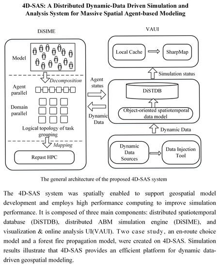
Figure 1.
The general architecture of the proposed 4D-SAS system.
Figure 1.
The general architecture of the proposed 4D-SAS system.
Figure 2.
The UML diagram of the spatially enabled classes in the DiSIME.
Figure 2.
The UML diagram of the spatially enabled classes in the DiSIME.
Figure 3.
The illustration of “agent parallel” decomposition (a) and “domain parallel with buffer size 1” decomposition (b).
Figure 3.
The illustration of “agent parallel” decomposition (a) and “domain parallel with buffer size 1” decomposition (b).
Figure 4.
The UML diagram of the object-oriented spatiotemporal data model in the DiSTDB.
Figure 4.
The UML diagram of the object-oriented spatiotemporal data model in the DiSTDB.
Figure 5.
An example of the st-object state records.
Figure 5.
An example of the st-object state records.
Figure 6.
The dynamic data ingestion supported by the data injection tool.
Figure 6.
The dynamic data ingestion supported by the data injection tool.
Figure 7.
An example XML format of one Transmission Item.
Figure 7.
An example XML format of one Transmission Item.
Figure 8.
The VAUI module for dynamic visualization and online analysis.
Figure 8.
The VAUI module for dynamic visualization and online analysis.
Figure 9.
The flow chart of the en-route driver choice model.
Figure 9.
The flow chart of the en-route driver choice model.
Figure 10.
The UML diagram of inherited classes in the en-route driver choice model.
Figure 10.
The UML diagram of inherited classes in the en-route driver choice model.
Figure 11.
The dynamic visualization of the en-route driver choice simulation (the red rectangle represents the flooded area, and the black points represent driving cars). The simulation results with different water-logging level: (a) Water-logging level is 0; (b) Water-logging level is 1; (c) Water-logging level is 2; (d) Water-logging level is 3.
Figure 12.
The total simulation time of the en-route driver choice model with different processor numbers.
Figure 12.
The total simulation time of the en-route driver choice model with different processor numbers.
Figure 13.
(a) The speedup and (b) parallel efficiency of the parallel en-route driver choice simulation.
Figure 13.
(a) The speedup and (b) parallel efficiency of the parallel en-route driver choice simulation.
Figure 14.
The change rules of the CA-based forest fire spread model.
Figure 14.
The change rules of the CA-based forest fire spread model.
Figure 15.
The UML diagram of inherited classes in the CA-based forest fire spread model.
Figure 15.
The UML diagram of inherited classes in the CA-based forest fire spread model.
Figure 16.
The dynamic visualization of the CA-based forest fire spread simulation with different wind speed (the black parts are burned area, and the red stands for the fire front). The simulation result after the same simulation ticks: (a) Wind speed is 0 km/h; (b) Wind speed is 5 km/h; (c) Wind speed is 10 km/h; (d) Wind speed is 15 km/h.
Figure 17.
The total simulation time of the CA-based forest fire spread model with different processor numbers.
Figure 17.
The total simulation time of the CA-based forest fire spread model with different processor numbers.
Figure 18.
(a) The speedup and (b) parallel efficiency of the parallel CA-based forest fire spread simulation.
Figure 18.
(a) The speedup and (b) parallel efficiency of the parallel CA-based forest fire spread simulation.
Table 1.
The detailed configuration of the cluster servers.
Table 1.
The detailed configuration of the cluster servers.
| Type | Manager | VAUI | DiSIME | DiSTDB |
|---|
| Number | 1 | 1 | 6 | 5 |
| CPU | Intel Xeon E5-2665 (2×8 cores, 2.40 GHz) | Intel Xeon E5-2620 (2×6cores, 2.00 GHz) | Intel Xeon E5-2620 (2×6 cores, 2.00 GHz) | Intel Xeon E5-2620 (2×6 cores, 2.00 GHz) |
| Memory | 32 GB(1333 MHz) | 32 GB(1333 MHz) | 32 GB(1333 MHz) | 32 GB(1333 MHz) |
| Hard disk | 250 GB (15 k rpm, SAS) | 500 GB (15 k rpm, SAS) | 500 GB (15k rpm, SAS) | 500 GB (15 k rpm, SAS) |
| Kernel | 3.10.0–123.el7.x86_64 | | 3.10.0–123.el7.x86_64 | 3.10.0–123.el7.x86_64 |
| OS | CentOS 7 | Windows 7 | CentOS 7 | CentOS 7 |
Table 2.
The total simulation time of the en-route driver choice model.
Table 2.
The total simulation time of the en-route driver choice model.
| Process Number | Time(s) | Speed up | Efficiency |
|---|
| 1 | 17,878.97 | 1.000 | 1.0000 |
| 2 | 9006.12 | 1.985 | 0.9925 |
| 4 | 4632.91 | 3.859 | 0.9665 |
| 6 | 3106.32 | 5.756 | 0.9648 |
| 8 | 2368.19 | 7.550 | 0.9437 |
| 10 | 1908.56 | 9.368 | 0.9368 |
| 12 | 1635.97 | 10.929 | 0.9108 |
| 14 | 1416.12 | 12.625 | 0.9018 |
| 16 | 1258.42 | 14.207 | 0.8879 |
Table 3.
The simulation time of the CA-based forest fire spread model.
Table 3.
The simulation time of the CA-based forest fire spread model.
| Process Number | Time(s) | Speedup | Efficiency |
|---|
| 1 | 2587.16 | 1.00 | 1.00 |
| 4 | 815.31 | 3.17 | 0.79 |
| 9 | 371.95 | 6.96 | 0.77 |
| 16 | 212.72 | 12.16 | 0.76 |
| 25 | 138.92 | 18.62 | 0.75 |
| 36 | 97.29 | 26.59 | 0.74 |
| 64 | 71.69 | 36.09 | 0.74 |
© 2016 by the authors; licensee MDPI, Basel, Switzerland. This article is an open access article distributed under the terms and conditions of the Creative Commons by Attribution (CC-BY) license (http://creativecommons.org/licenses/by/4.0/).


