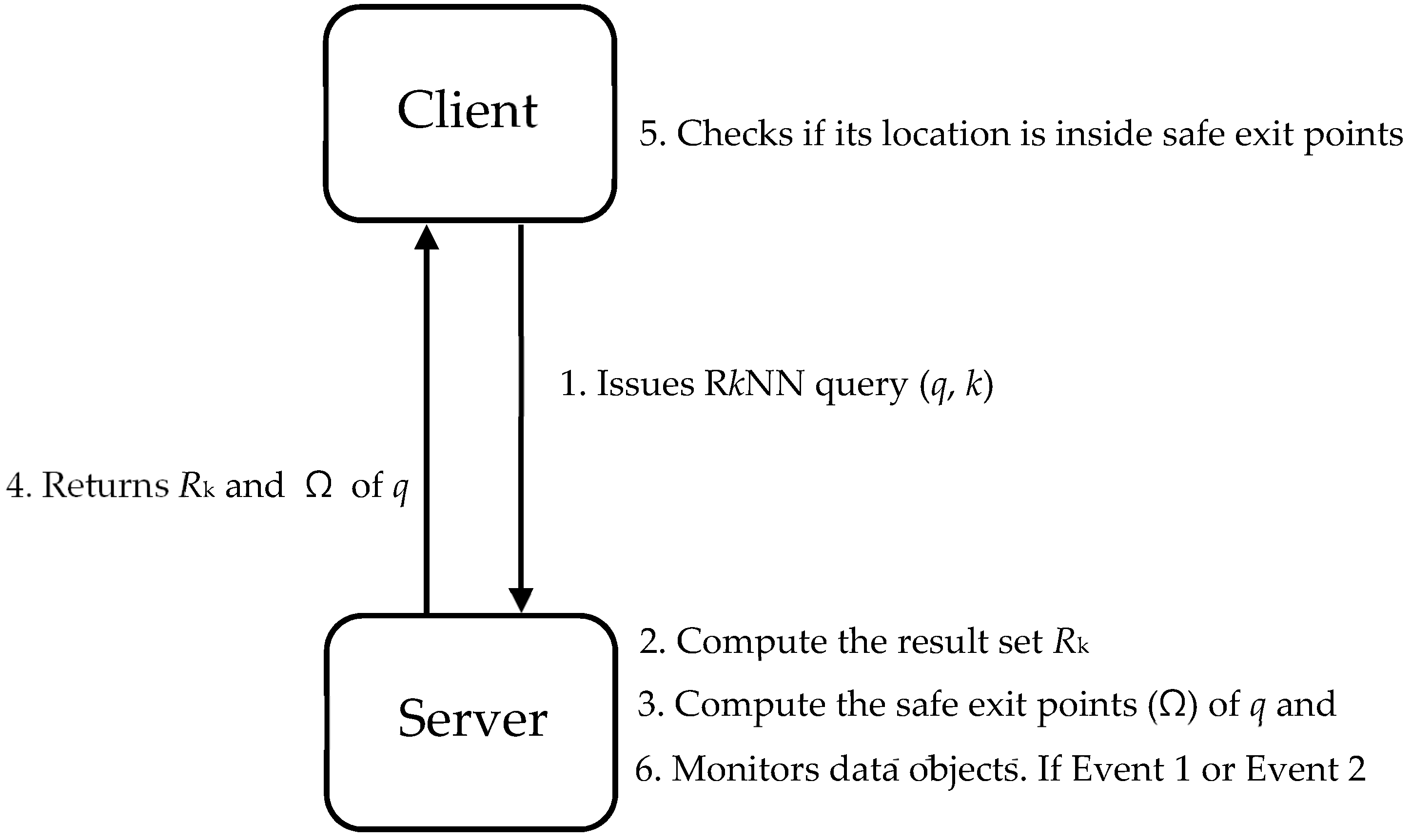
In this section, we present a new safe exit algorithm that addresses the issue for moving RkNN queries and moving objects in a road network. Algorithm 1 depicts the skeleton of the proposed safe exit algorithm for computing safe regions. It consists of three phases: (1) determining the useful objects that can contribute to the safe region; (2) computing the influence region of the useful objects; (3) computing the safe exit points for the query objects.
4.1.1. Determining Useful Objects
This phase aims at determining potential objects that could contribute to the computation of the safe region. The goal is to retrieve a small set of data objects to reduce the computation overhead. In our study, the data objects are divided into two categories: answer objects (denoted by ) and non-answer objects (denoted by ).
Definition 1. An object o is called an answer object if where o′ is any other object in the road network. Similarly, we can generalize this definition for RkNN: an object o is called an answer object if , where ok+1 is the (k + 1)th NN object of o. That is, we can say that all answer objects are RkNNs of query q, therefore, .
Definition 2. An object o is called a non-answer object if , where o′ is any other object in the road network.
Similarly, we can generalize this definition for RkNN: an object o is called a non-answer object if , where ok is the kth NN object of o. That is, we can say that all non-answer objects are not RkNN of query q, therefore, .
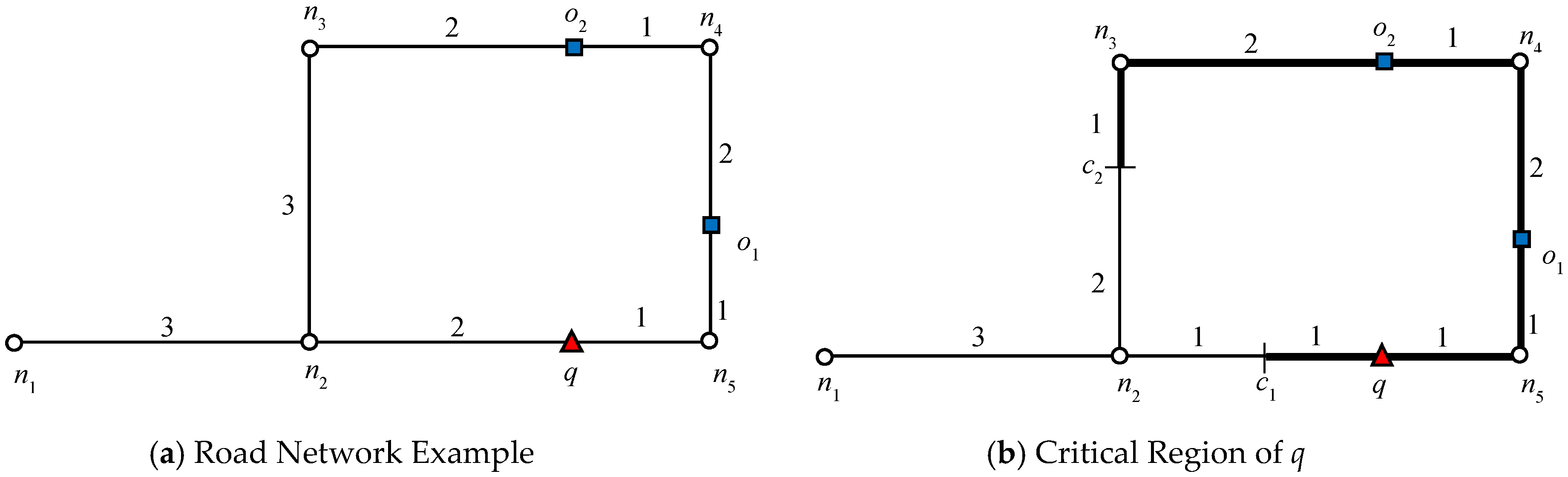
A simple method for retrieving the set is to traverse the network from q, and for each data object encountered, issue a nearest-neighbor query. If , q is the closest object to o. Consequently, However, this approach must evaluate all the data objects because the size of is not fixed and the road network may contain points that are far from q. To avoid unnecessary road network exploration, we present the pruning lemma.
Before presenting the lemma, it is necessary to define closed nodes. A node
n is called a closed node if there exists an object
o such that
. The object
o is called a blocking object because it causes node
n to be a closed node. In
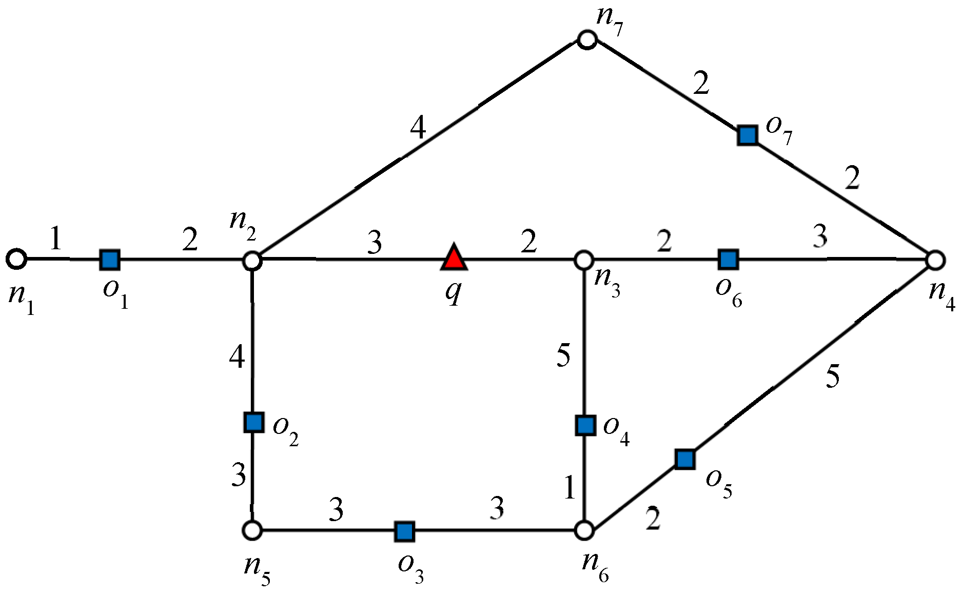
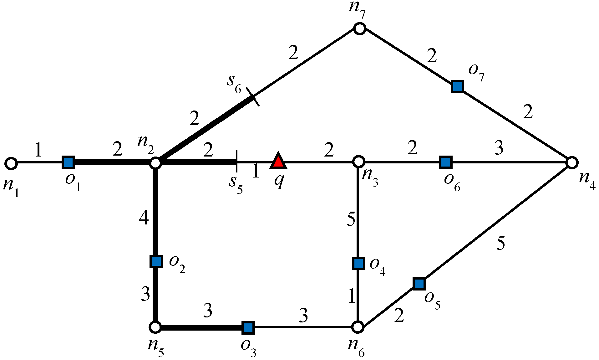
Figure 1, node
n2 is a closed node because
, which makes
o1 a blocking object.
Lemma 1. An object o cannot be the RNN of q if the shortest path between q and o contains a closed node with a blocking object o′, where
Proof. Let us assume that there exists a closed node n on the shortest path between o and q. The shortest distance between o and q is . Let o′ be the blocking object and . As we know therefore, . Therefore, o cannot be an RNN of q.
In
Figure 1, the data object
o2 cannot be an RNN of
q because the shortest distance between
o2 and
q passes through
n2. Because
and
, data object
o1 is closer to
o2 than
q. The above lemma can be easily extended to R
kNN. An object
o cannot be the R
kNN of
q if the shortest path between
q and
o contains a node
n and there exist
k data objects
o′ such that for every object
o′,
, where
Algorithm 2 presents the pseudo code for determining the answer objects. CORE-X traverses the network around q in a similar fashion to Dijkstra’s algorithm; using Lemma 1, it eliminates the nodes that may not lead to RNNs. The algorithm begins by exploring the active edge where query object q is located and expands the network in an increasing order of distance from the query object q. Each entry in the queue has the form 〈〉, where pa indicates the anchor point on the edge. For an active edge, q becomes the anchor point. Otherwise, neither of the boundary nodes of the edge, i.e., or , becomes the anchor point. If the desired number of answer objects is not found on an active edge, the edges adjacent to the boundary nodes are enqueued. The edges are popped in an increasing order of distance from q. The traversal of the edges is terminated when the queue is exhausted. Line 4 initializes a queue by inserting the active edge. If an edge contains a data object o, we must verify whether . Thus, the algorithm issues a verify(o, k, q) query (Line 10). The verification query checks if q is among the kNNs of data object o by applying a range-NN query around object o with the range set to . If , o is the RkNN of q. Therefore, o is added to the result set Rk (Line 12). If the edge does not contain any data object o, the algorithm continues its expansion and enqueues the adjacent edges of the boundary node.
| Algorithm 2: Answer object(q, k) |
| Input: q: query location, k: integer number |
| Output: Rk: query result (answer objects) |
| 1: | | /* queue is a priority queue with edges ordered by distance to q*/ |
| 2: | | /* set of answer objects*/ |
| 3: | | /*stores information of visited edges */ |
| 4: | queue.push(q,edgeactive) | /* edgeactive indicates active edge */ |
| 5: | While queue is not empty do |
| 6: | | |
| 7: | | If then |
| 8: | | | |
| 9: | | | | If edge contains a data object o |
| 10: | | | | | kNN(o): verify(o, k, q) |
| 11: | | | | | If q discovered by verification |
| 12: | | | | | | |
| 13: | | | | Else |
| 14: | | | | | |
| 15: | End while |
| 16: | Return Rk |
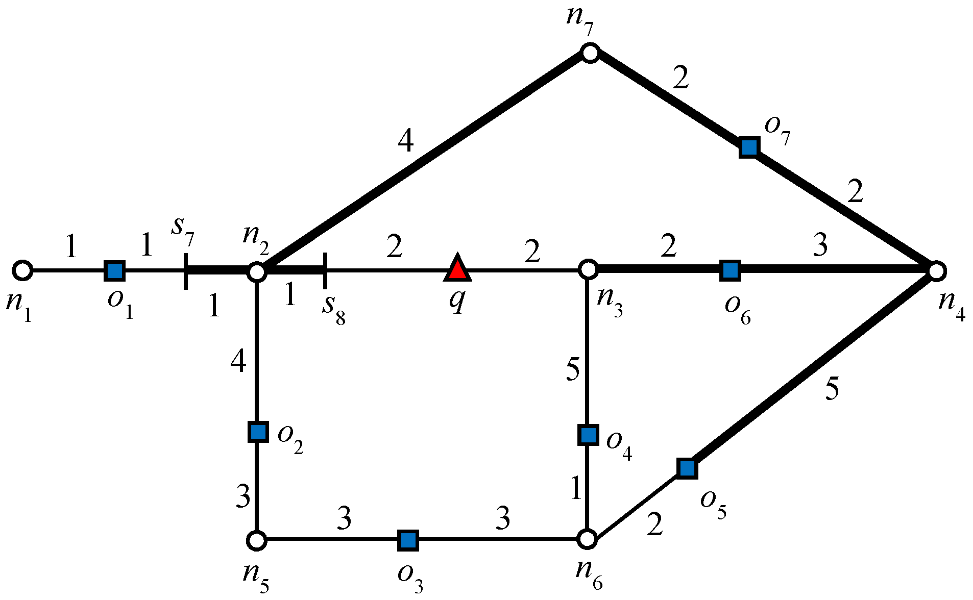
Let us consider the example presented in
Figure 1, where query
q requested one RNN (
k = 1). We will consider this example throughout this section. The algorithm starts expansion from the active edge, which is
. Because no data object is discovered on that edge, edges adjacent to the boundary nodes will be added to the queue. The edges adjacent to the closest boundary node are enqueued first. Therefore, edges
are enqueued. Data object
o6 is first discovered on
, which triggers the verification query verify(
o6, 1,
q). Because
q = NN(
o6),
o6 is added to the result set
Rk. Recall that by Lemma 1, node
n4 is a closed node with object
o6 as the blocking object. Therefore, all the other objects for which the shortest distance passes through
n4 except
o6 are automatically pruned. Then, data object
o4 is discovered on
, by verification of
o4,
; therefore, the search also terminates in this direction. Next, the edges adjacent to
n2 are added to the queue,
and data object
o1 is retrieved on
. The data object
o1 is verified and added to the result set because
q = NN(
o1). The search terminates as no further expansion is required in this direction because node
n2 is a closed node.
Next, we determine the non-answer objects that can contribute to the safe region. Useful non-answer objects are objects for which any . In other words, are RNNs of answer objects. RNNs of Useful Objects (UO) can be determined by the same algorithm making these modifications: (1) the anchor point is o+ instead of q and (2) verification query verify(o, k, q) is modified to verify(o, k, o+). The algorithm reuses the results of the range-NN queries issued at the data objects to avoid multiple verification of the same data objects. When the computation is completed, the cached query results are removed to reduce the memory consumptions.
Finally, we can conclude that useful objects are: (1) all answer objects and (2) RNNs of answer objects. Now, let us determine the UO objects for
k = 2 in the given example in
Figure 1. For explanation,
Table 2 displays the
kNNs of each data object.
.
From
Table 2 it is clear that
o1 and
o6 are both answer objects because
q is one of the 2NNs. Now, from the non-answer objects, we can see that
o2 is the RNN of
o1 because
o1 = 2NN(
o2). Similarly,
o7 is the RNN of
o6. Hence, the set of useful objects is
. Data objects
o3,
o4, and
o5 have been pruned.
4.1.2. Computing Influence Region for Useful Objects
After we retrieve the set of useful objects, the next step is to compute the influence region of the answer and non-answer objects.
Influence Region of Answer Objects
The influence region of the answer objects is defined as:
Here,
ok+1 denotes the (
k+1)th nearest neighbor of
o. By definition, the influence region of the answer objects contains all the points for which
. That is, it contains all of the points where object
o remains
.
The influence region of answer objects can be computed by exploring the network around the answer object in a manner similar to that explained in
Section 4.1.1. The exploration terminates with the discovery of the (
k+1)th nearest neighbor of the answer object. The influence region will be indicated by
range(
o,
d), where
d is the
.
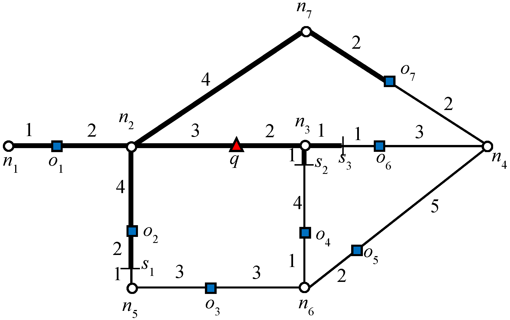
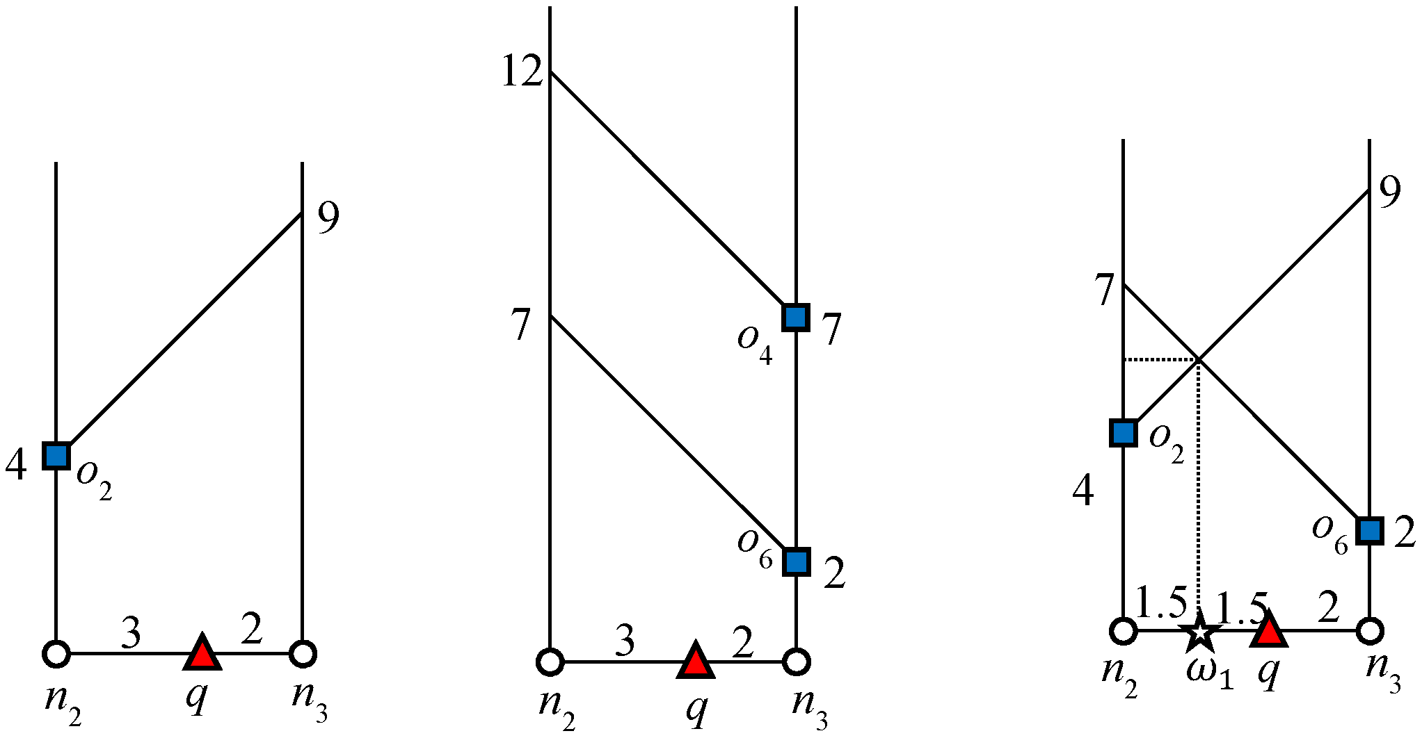
Figure 3 indicates the influence region of object
o1 for the example scenario discussed above. The expansion of the road network starts from
o1 until it finds
ok+1, which is 3NN in this example. Object
o7 is 3NN of
o1 and
. The algorithm will issue a
query that marks all of the points as the influence region of
o1 as shown in
Figure 3. Similarly, the influence region of
is indicated in
Figure 3. The data object
o4 is the 3NN of
o6 and
Therefore, the
query marks all the points within the distance of “7” from
. The bold lines in
Figure 3 and
Figure 4 indicate the influence region of
and
, respectively.
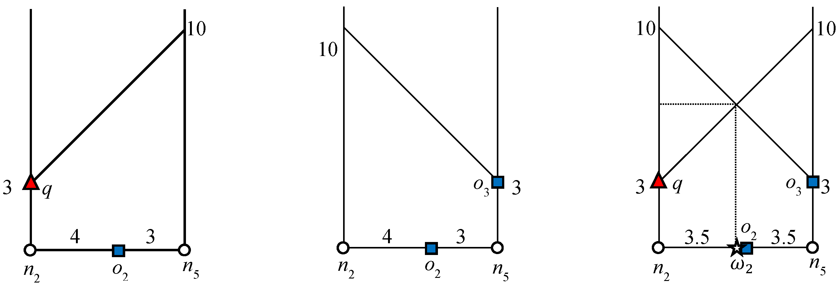
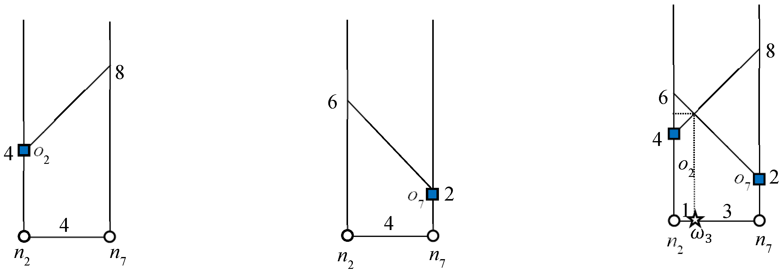
Influence Region of Non-Answer Objects
The influence region of non-answer objects is defined as:
The influence region of non-answer objects can be computed from the distance between the non-answer object and kth object. Here ok denotes the kth nearest neighbor of o. In other words, the influence region of non-answer objects contains all the points where object o remains . The influence region of non-answer objects is computed in the same manner as the influence region of answer objects, the only difference is that the algorithm explores and computes the distance to the kNN object instead of (k + 1)NN.
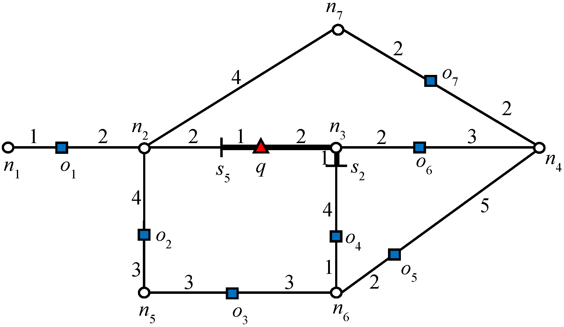
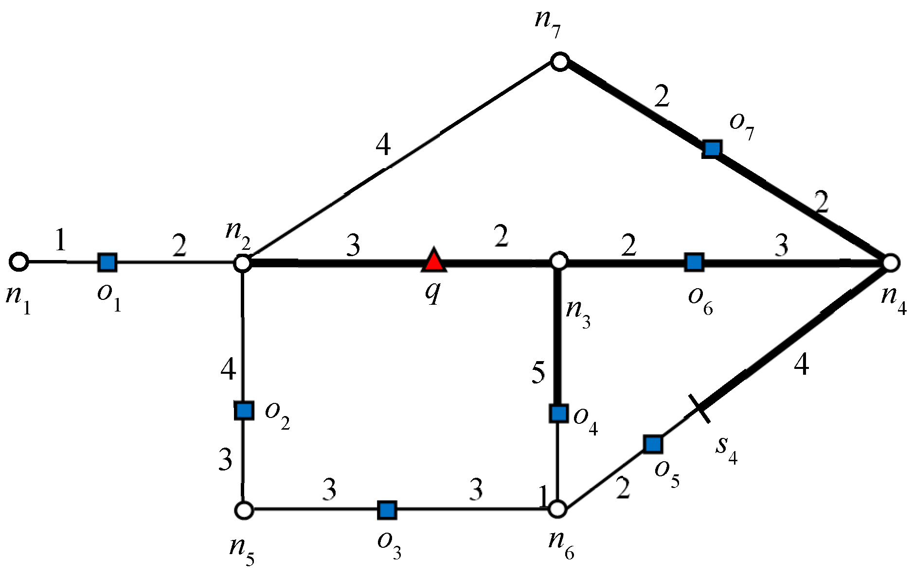
Consider object
o7 in
Figure 1: 2NNs of
with weights (5, 7). In this example,
o5 is the second NN of
and
. Therefore, the influence region of object
o7 is “7” units from
o7 in every connected direction. Similarly, we can compute the influence region of
o2. The bold lines in
Figure 5 and
Figure 6 indicate the influence region of
o2 and
o7, respectively. The NNs for answer objects change when the query object moves outside the influence region, whereas in the case of non-answer objects, the result changes when the query object moves inside an influence region. That is, the NNs of the answer object remain the same until the query object lies inside the influence region and for non-answer objects, the NNs remain the same until query object lies outside the influence region. Note that once an influence region is computed, it remains valid as long as
q and UO lie within their respective safe regions. Hence, recomputation of the influence region is only required when either
q or UO leave their respective safe regions.
Algorithm 3 computes the influence region of answer objects and non-answer objects.
| Algorithm 3: Computation of Influence Region (, , k) |
| Input: : answer objects set, : non-answer objects set, k: integer number |
| Output: influence region of answer objects, influence region of non-answer objects |
| 1: | , |
| /* Influence Region of answer objects */ |
| 2: | For each do |
| 3: | | Expand the road network until ok+1; |
| 4: | | |
| 5: | | Mark range(o, d); |
| 6: | | ; |
| 7: | End for |
| /* Influence Region of non-answer objects */ |
| 8: | For each do |
| 9: | | Expand the road network until ok; |
| 10: | | ; |
| 11: | | Mark range(o, d); |
| 12: | | ; |
| 13: | End for |
| 14: | Return and |


