
Evaluation of River Network Generalization Methods for Preserving the Drainage Pattern


Abstract
:1. Introduction
2. Related work
2.1. Tributary Selection Methods
2.2. Generalized River Network Quality Assessment
3. Assessment of Drainage Pattern Preservation in River Generalization
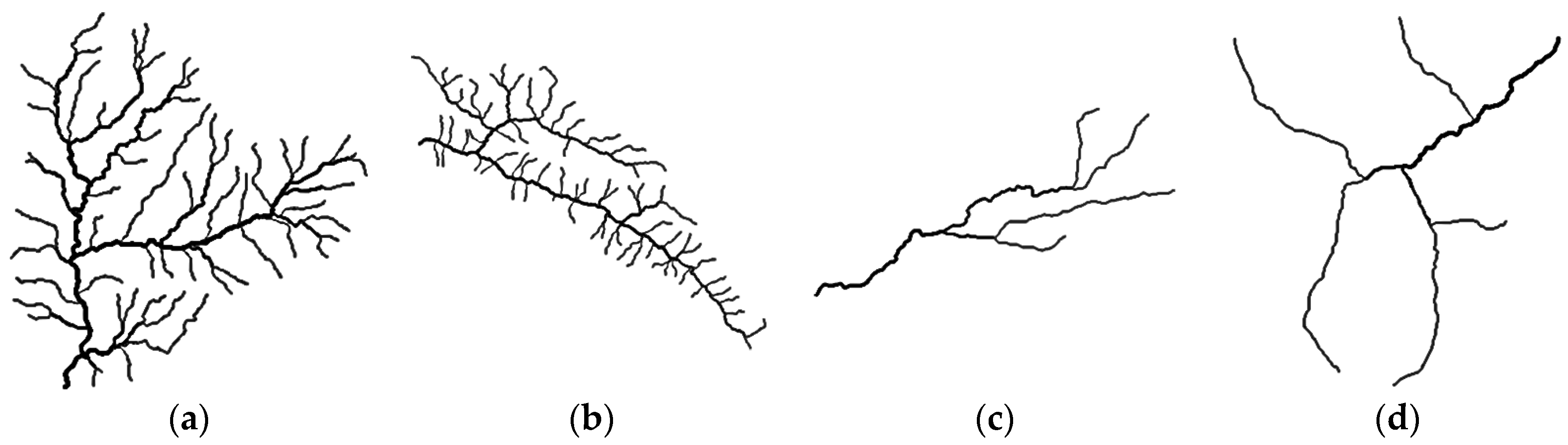
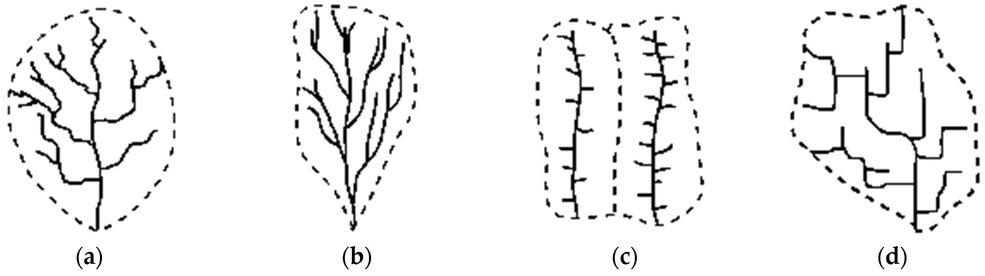
3.1. Drainage Pattern Classification
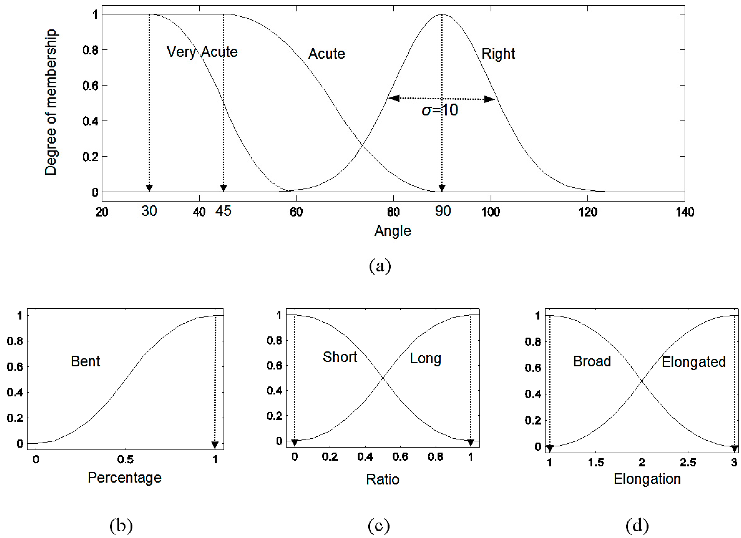
- α IS acute/very acute/right,
- β IS bent,
- γ IS long/short,
- δ IS broad/elongated.
- IF (α IS acute) AND (δ IS broad) THEN pattern IS dendritic.
- IF (α IS very acute) AND NOT (β IS bent) AND (γ IS long) AND (δ IS elongated) THEN pattern IS parallel.
- IF (α IS right) AND NOT (β IS bent) AND (γ IS short) AND (δ IS elongated) THEN pattern IS trellis.
- IF (α IS right) AND (β IS bent) THEN pattern IS rectangular.
3.2. Evaluation of Generalized Networks
- Generalize the network by applying a stream selection method.
- Evaluate the pattern of all drainages in the new network.
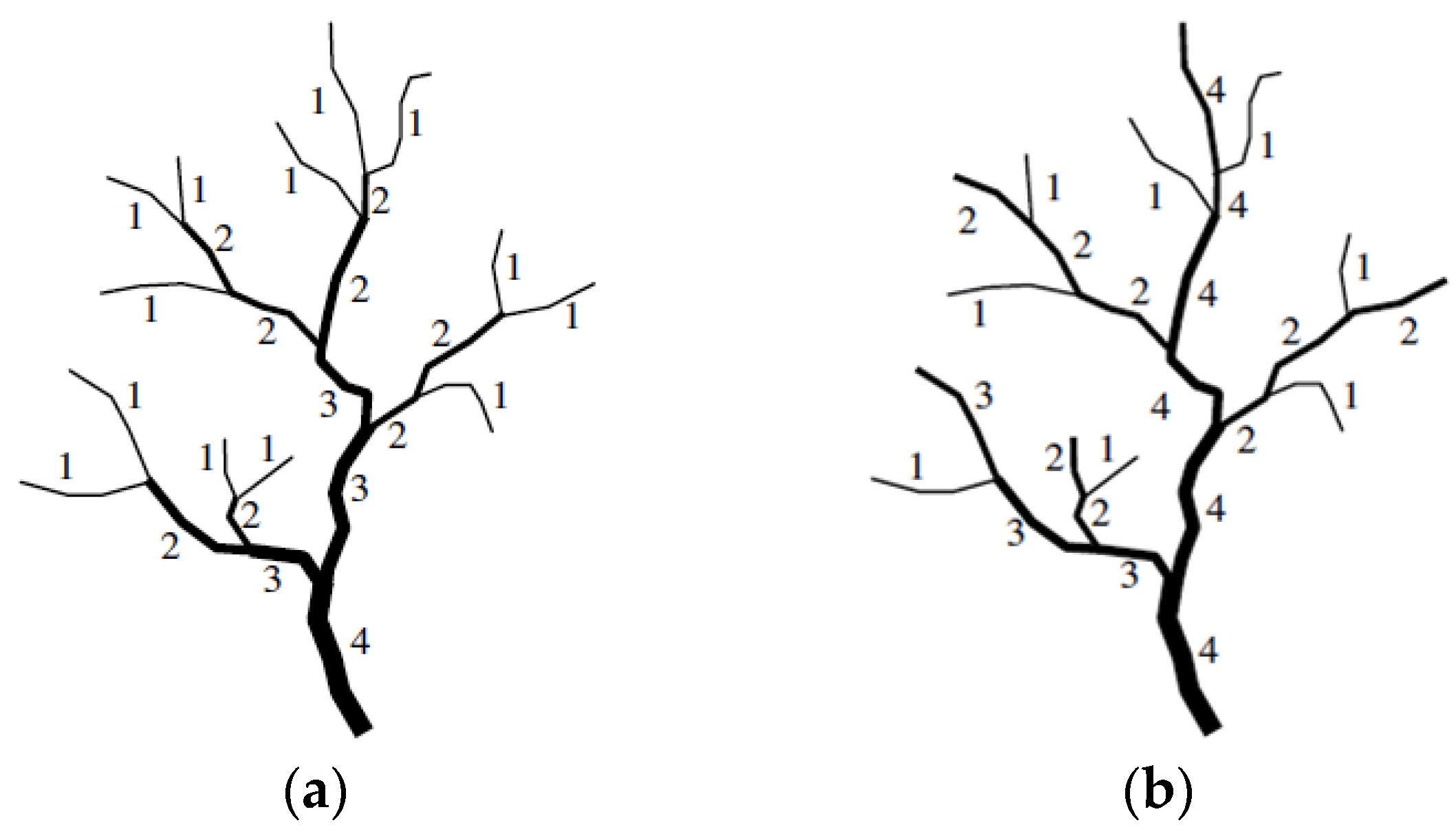
- For each drainage in the simplified network, find its equivalent drainage in the original network according to the stream ID, then compare them to check if the pattern has been preserved.
4. Experimentation Design
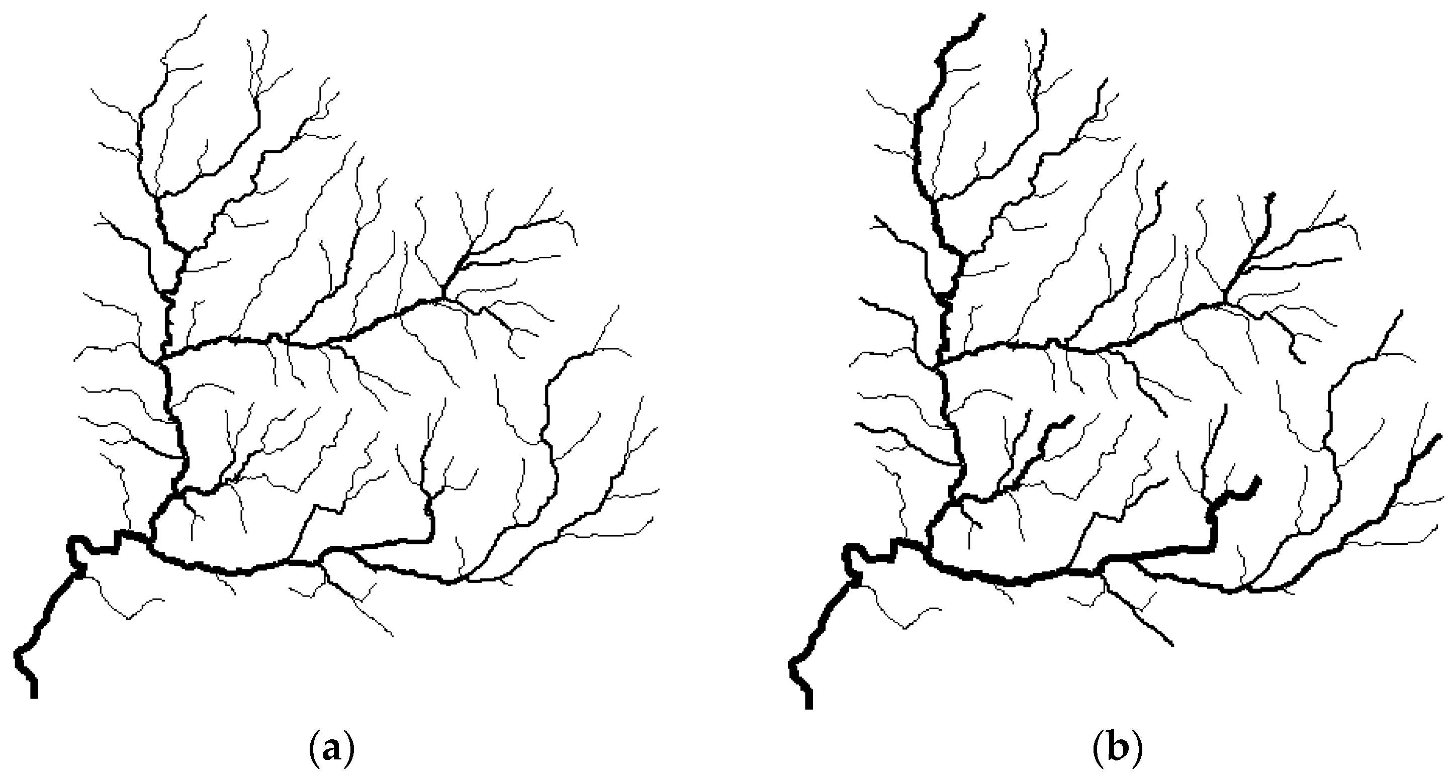
4.1. Tributary Selection by Stroke and Length
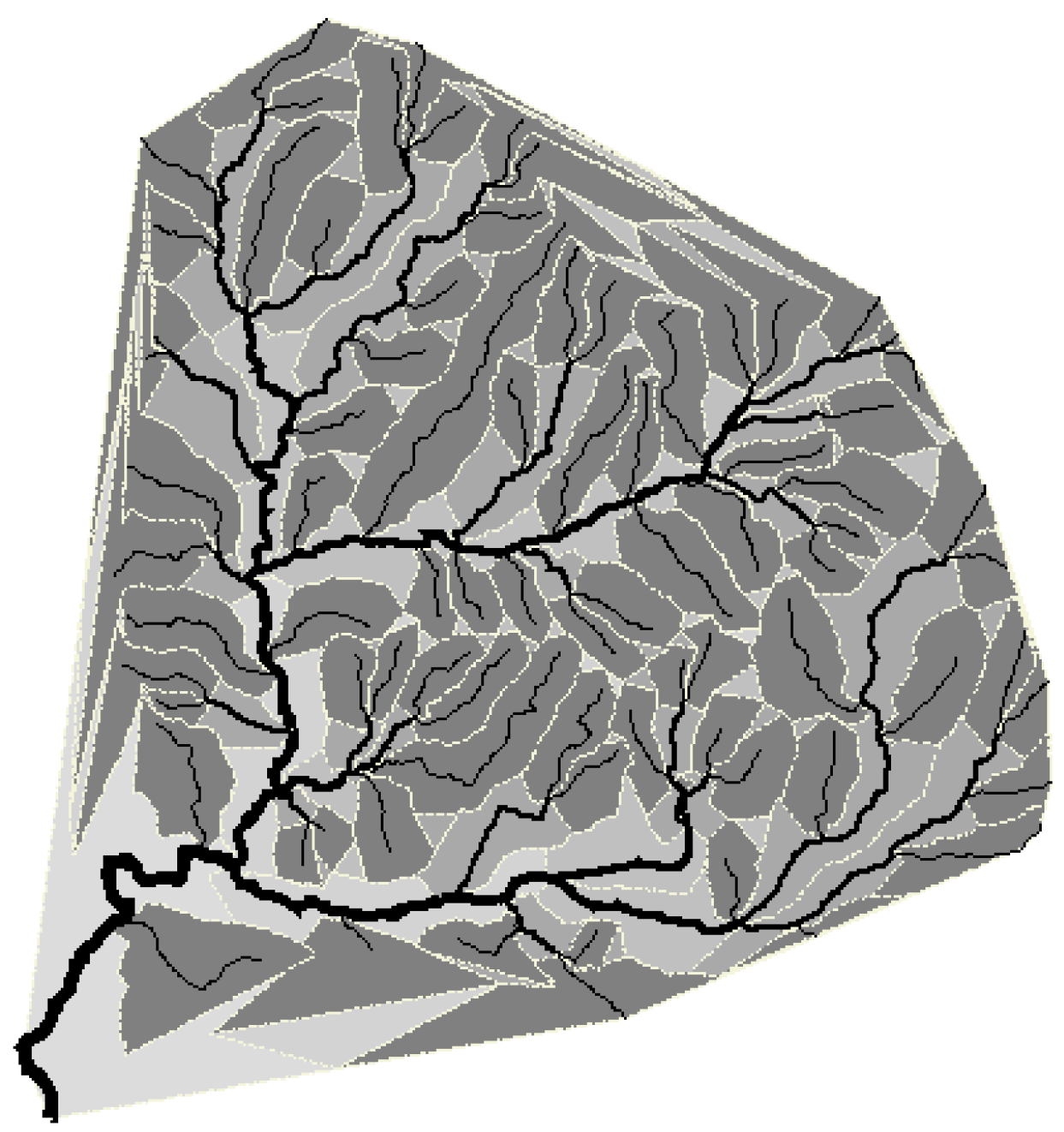
4.2. Tributary Selection by Watershed Partitioning
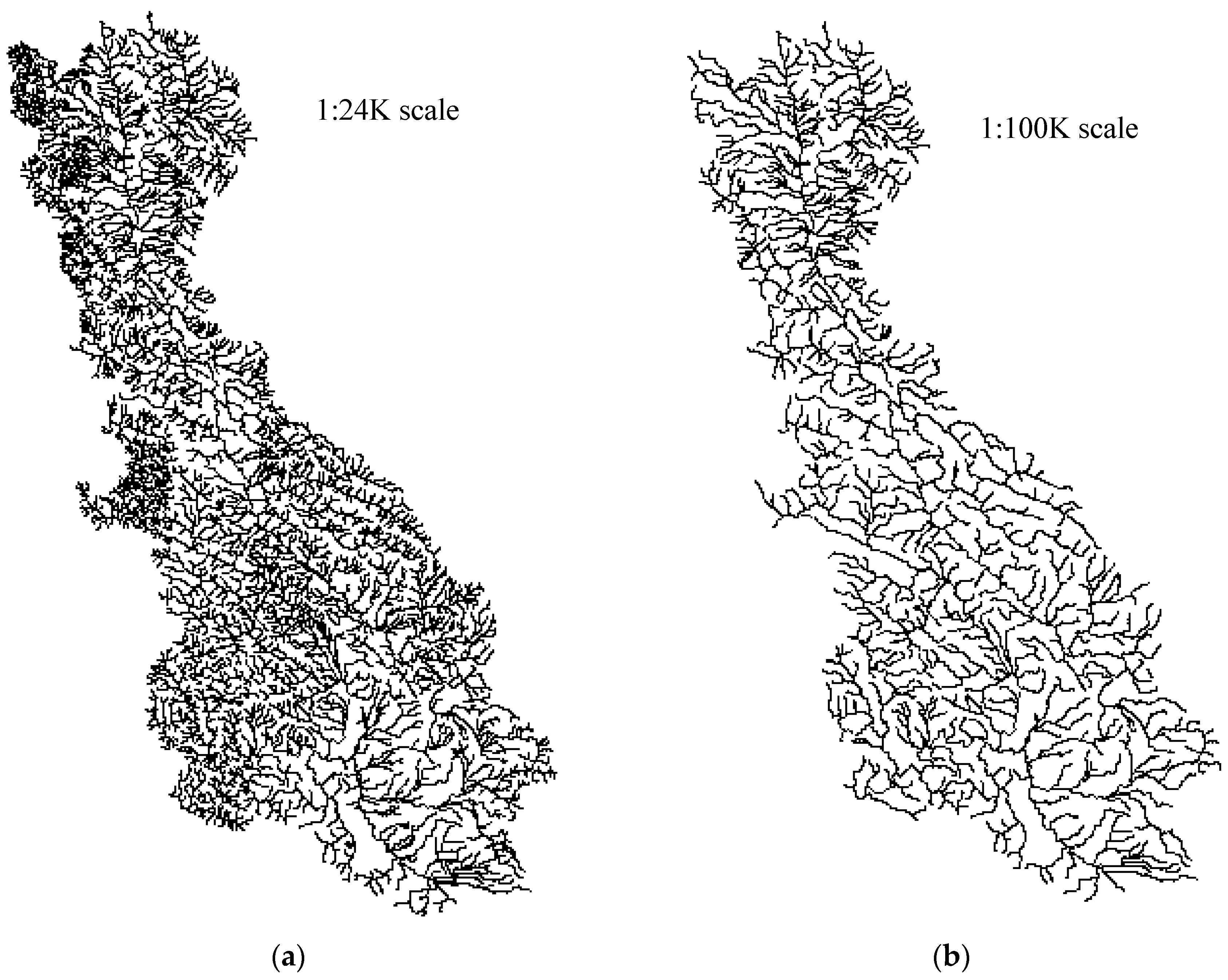
4.3. Testing Data
4.4. MF Parameter Settings
5. Experiment results
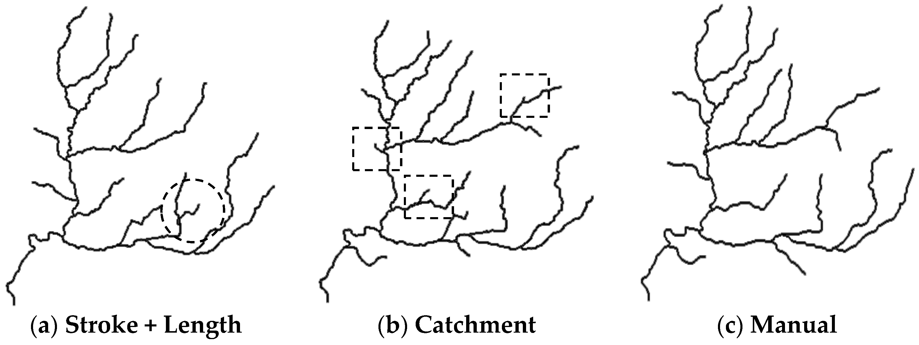
5.1. Case Studies in Russian River
5.1.1. Case 1: A Dendritic River Network
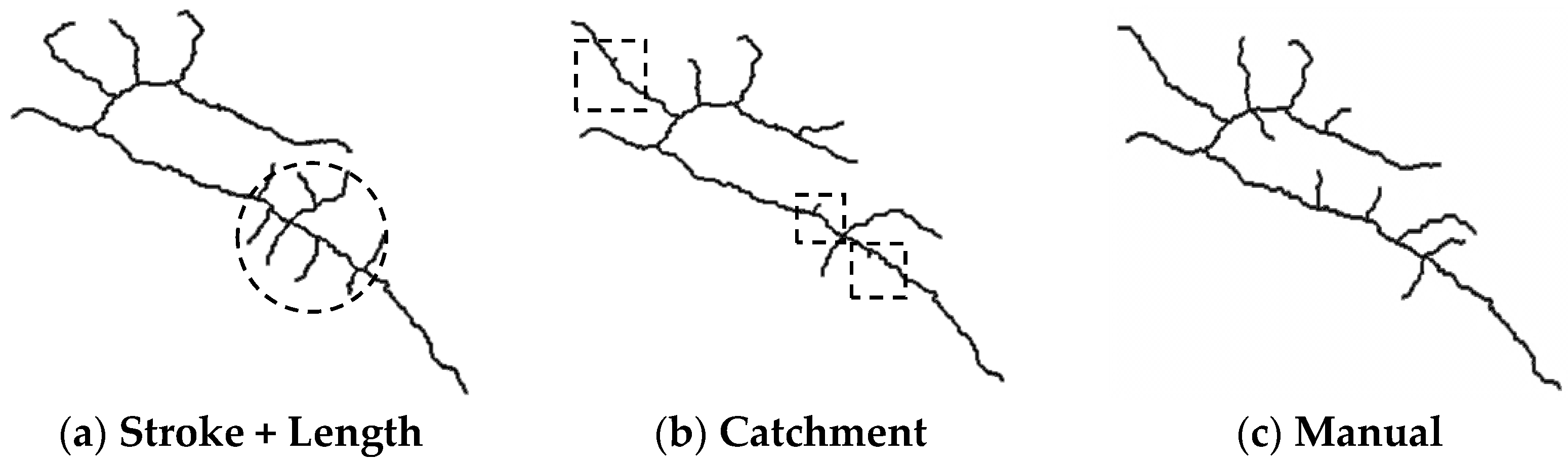
5.1.2. Case 2: A Trellis River Network
5.2. Evaluation Results in the Russian River
5.3. Discussion
- In general, the evaluation method based on the membership degree of a fuzzy rule for a drainage pattern is useful. From a large scale to a small scale, to a generalized river network, the drainage pattern preserves better if the membership value is high. However, sometimes, the membership value will be not so robust at small scales, especially when there are not enough river segments left because proposed indicators, such as average junction angle (α), bent tributaries percentage (β), and average length ratio (γ), are statistical features.
- By evaluating generalized river networks from the point of drainage patterns, the method based on stroke and length is better than based on watershed partitioning. In addition, networks generalized manually are always with high membership values and preserve a good drainage pattern. A good generalized result does not only depend on one or two factors; many factors such as tributary spacing and balance are involved in manual generalization process.
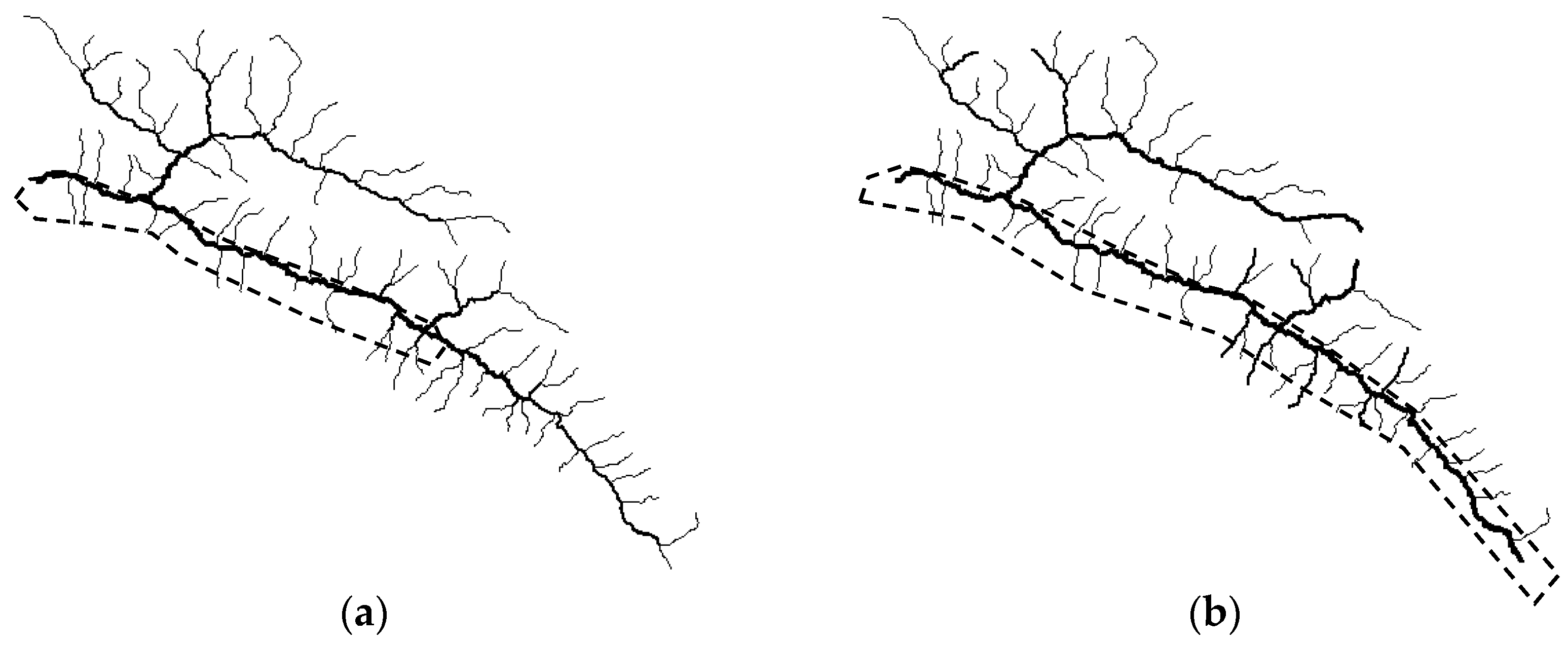
- One limitation is that this research only focuses on the evaluation of the drainage pattern. Some other aspects simply cannot be assessed by the membership value. For example, for network (f) in Table 9 at the 1:500K scale, although the membership value is 0.896, much greater than (g), it is not an ideal result as the tributaries in the dashed circle are crowded together in Table 10.
- Another limitation is that the evaluation method is more reliable and accurate in source river networks with order 3 or higher, but higher order is not always better because sub-networks can be classified in different patterns inside a large river network. A small river network with order 2 does not have enough river segments to provide robust indicators.
6. Summary
Acknowledgments
Author Contributions
Conflicts of Interest
References
- Chen, Y.; Wilson, J.P.; Zhu, Q.; Zhou, Q. Comparison of drainage-constrained methods for DEM generalization. Comput. Geosci. 2012, 48, 41–49. [Google Scholar] [CrossRef]
- Li, Z.; Zhu, Q.; Gold, C. Digital Terrain Modeling: Principles and Methodology; CRC Press: Boca Raton, FL, USA, 2010. [Google Scholar]
- Génevaux, J.-D.; Galin, É.; Guérin, E.; Peytavie, A.; Beneš, B. Terrain generation using procedural models based on hydrology. ACM Trans. Graph. 2013, 32, 1–10. [Google Scholar] [CrossRef]
- Ai, T.; Liu, Y.; Chen, J. The hierarchical watershed partitioning and data simplification of river network. In Progress in Spatial Data Handling; Riedl, A., Kainz, W., Elmes, G.A., Eds.; Springer: Berlin/Heidelberg, Germany, 2006; pp. 617–632. [Google Scholar]
- Buttenfield, B.P.; Stanislawski, L.V.; Brewer, C.A. Multiscale representations of water: Tailoring generalization sequences to specific physiographic regimes. In Proceedings of the GIScience 2010, Zurich, Switzerland, 15–17 September 2010; pp. 14–17.
- Stanislawski, L.V. Feature pruning by upstream drainage area to support automated generalization of the United States National Hydrography Dataset. Comput. Environ. Urban Syst. 2009, 33, 325–333. [Google Scholar] [CrossRef]
- Bard, S.; Ruas, A. Why and how evaluating generalised data? In Developments in Spatial Data Handling; Springer: Berlin/Heidelberg, Germany, 2005; pp. 327–342. [Google Scholar]
- Twidale, C.R. River patterns and their meaning. Earth-Sci. Rev. 2004, 67, 159–218. [Google Scholar] [CrossRef]
- Ritter, M.E. The Physical Environment: An Introduction to Physical Geography. Available online: http://www.earthonlinemedia.com/ebooks/tpe_3e/title_page.html (accessed on 28 November 2016).
- Charlton, R. Fundamentals of Fluvial Geomorphology; Routledge: London, UK, 2007. [Google Scholar]
- Fagan, S.D.; Nanson, G.C. The morphology and formation of floodplain-surface channels, Cooper Creek, Australia. Geomorphology 2004, 60, 107–126. [Google Scholar] [CrossRef]
- Li, Z. Algorithmic Foundation of Multi-Scale Spatial Representation; CRC: Boca Raton, FL, USA, 2007. [Google Scholar]
- Mackaness, W.; Edwards, G. The importance of modelling pattern and structure in automated map generalisation. In Proceedings of the Joint ISPRS/ICA Workshop on Multi-Scale Representations of Spatial Data, Ottawa, ON, Canada, 7–8 July 2002; pp. 7–8.
- Zhang, L.; Guilbert, E. Automatic drainage pattern recognition in river networks. Int. J. Geogr. Inf. Sci. 2013, 27, 2319–2342. [Google Scholar] [CrossRef]
- Topfer, F.; Pillewizer, W. The principles of selection. Cartogr. J. 1966, 3, 10–16. [Google Scholar] [CrossRef]
- Wilmer, J.; Brewer, C. Application of the radical law in generalization of national hydrography data for multiscale mapping. In Proceedings of a Special Joint Symposium of ISPRS Technical Commission IV & AutoCarto in conjunction with ASPRS/CaGIS 2010 Fall Specialty Conference, Orlando, FL, USA, 15–19 November 2010.
- Mazur, R.E.; Castner, H.W. Horton’s ordering scheme and the generalisation of river networks. Cartogr. J. 1990, 27, 104–112. [Google Scholar] [CrossRef]
- Burghardt, D.; Duchene, C.; Mackaness, W. Abstracting Information in a Data Rich World: Methodologies and Applications of Map Generalization; Springer: Berlin, Germany, 2014. [Google Scholar]
- Richardson, D.E. Automated Spatial and Thematic Generalization Using a Context Transformation Model: Integrating Steering Parameters, Classification and Aggregation Hierarchies, Reduction Factors, and Topological Structures for Multiple Abstractions; R&B Publications: Kanata, ON, Canada, 1993. [Google Scholar]
- Thomson, R.C.; Brooks, R. Efficient generalization and abstraction of network data using perceptual grouping. In Proceedings of the 5th International Conference on Geo-Computation, University of Greenwich, London, UK, 2000; pp. 23–25.
- Touya, G. River network selection based on structure and pattern recognition. In Proceedings of ICC2007, Moscow, Russia, 4–10 August 2007; pp. 4–9.
- Wolf, G.W. Weighted surface networks and their application to cartographic generalization. In Visualisierungstechniken und Algorithmen; Springer: Berlin, Germany, 1988; Volume 182, pp. 199–212. [Google Scholar]
- Wu, H. Structured approach to implementing automatic cartographic generalization. In Prceedings of the 18th ICC, Stockholm, Sweden, 23–27 June 1997.
- Zhai, R.J.; Wu, F.; Deng, H.; Tan, X. Automated elimination of river based on multi-objective optimization using genetic algorithm. J. China Univ. Min. Technol. 2006, 35, 403–408. (In Chinese) [Google Scholar]
- Stanislawski, L.V.; Buttenfield, B.P. Hydrographic generalization tailored to dry mountainous regions. Cartogr. Geogr. Inf. Sci. 2011, 38, 117–125. [Google Scholar] [CrossRef]
- Stanislawski, L.V. Development of a knowledge-based network pruning strategy for automated generalisation of the United States National Hydrography Dataset. In Proceedings of the 11th ICA Workshop on Generalization and Multiple Representation, Montpellier, France, 20–21 June 2008.
- Savino, S.; Rumor, M.; Zanon, M. Pattern Recognition and Typification of Ditches. In Advances in Cartography and GIScience; Ruas, A., Ed.; Springer: Berlin/Heidelberg, Germany, 2011; Volume 1, pp. 425–437. [Google Scholar]
- Muller, J.; Weibel, R.; Lagrange, J.; Salge, F. Generalization: State of the art and issues. In GIS and Generalization: Methodology and Practice; Taylor & Francis: London, UK, 1995; pp. 3–17. [Google Scholar]
- Weibel, R.; Dutton, G. Generalising spatial data and dealing with multiple representations. In Geographical Information Systems: Principles, Techniques, Management and Applications; Longley, P., Goodchild, M., Maguire, D., Rhind, D., Eds.; Springer: Berlin/Heidelberg, Germany, 1999; pp. 125–155. [Google Scholar]
- Weibel, R. Three essential building blocks for automated generalization. In GIS and Generalization: Methodology and Practice; Taylor & Francis: London, UK, 1995; pp. 56–69. [Google Scholar]
- Joao, E. Causes and Consequences of Map Generalisation; Taylor & Francis: London, UK, 1998. [Google Scholar]
- Mackaness, W.; Ruas, A. Evaluation in the map generalisation process. In Generalisation of Geographic Information: Cartographic Modelling and Applications; Elsevier: Amsterdam, The Netherlands, 2007; pp. 89–111. [Google Scholar]
- Bard, S. Quality assessment of cartographic generalisation. Trans. GIS 2004, 8, 63–81. [Google Scholar] [CrossRef]
- Stanislawski, L.V.; Buttenfield, B.P.; Doumbouya, A. A rapid approach for automated comparison of independently derived stream networks. Cartogr. Geogr. Inf. Sci. 2015, 42, 435–448. [Google Scholar] [CrossRef]
- Skopeliti, A.; Tsoulos, L. A methodology for the assessment of generalization quality. In Proceedings of the Fourth ACI Workshop on Progress in Automated Map Generalization, Beijing, China, 2–4 August 2001.
- Zhang, X. Automated Evaluation Of Generalized Topographic Maps. Ph.D. Thesis, The University of Twente, Enschede, The Netherlands, 4 October 2012. [Google Scholar]
- Schumm, S.A. The Fluvial System; Wiley: New York, NY, USA, 1977. [Google Scholar]
- Zadeh, L.A. Fuzzy sets. Inf. Control 1965, 8, 338–353. [Google Scholar] [CrossRef]
- Thomson, R.C. The stroke concept in geographic network generalization and analysis. In Progress in Spatial Data Handling; Springer: Berlin/Heidelberg, Germany, 2006; pp. 681–697. [Google Scholar]
- Braden, B. The surveyor’s area formula. Coll. Math. J. 1986, 17, 326–337. [Google Scholar] [CrossRef]
- USEPA; USDOI. Standards for National Hydrography Dataset; United States Environmental Protection Agency and United States Department of the Interior, United States Geological Survey: Reston, VA, USA, 1999.


| Indicator | Description | Illustration |
|---|---|---|
| Average junction angle (α) | The angle is composed by upper tributaries. α is given by the average value of angles measured at all junctions in a river network. |  |
| Bent tributaries percentage (β) | Sinuosity is the ratio of the channel length to the valley length [37]. A channel is considered to be bent if sinuosity ≥ 1.5 [9]. β is calculated as the number of bent tributaries divided by the total number of tributaries. |  |
| Average length ratio (γ) | Length ratio is the ratio of the tributary length to the main stream length. γ is the average value of all length ratios in a network. |  |
| Catchment elongation (δ) | A ratio of the depth to the breadth of a catchment. |  |
| No. | Approaches | Methods |
|---|---|---|
| I | Hierarchy | Stroke + Length |
| II | Watershed partitioning (Catchment) | |
| III | Manual |
| Predicate | MF |
|---|---|
| α IS acute | |
| α IS very acute | |
| γ IS short | |
| δ IS broad | |
| α IS right | |
| β IS bent | |
| γ IS long | |
| δ IS elongated |
| Method | Indicator | Membership Value | |||||||
|---|---|---|---|---|---|---|---|---|---|
| α | β | γ | δ | D | P | T | R | ||
| Stroke + Length | (a) | 59.19° | 4.00% | 1.10 | 1.20 | 0.801 | 0.002 | 0 | 0.003 |
| Catchment | (b) | 61.52° | 8.57% | 0.58 | 1.16 | 0.730 | 0 | 0.013 | 0.015 |
| Manual | (c) | 56.52° | 10.34% | 0.64 | 0.99 | 0.869 | 0 | 0 | 0.004 |
| 1:24K | Method | Scale | ||||
|---|---|---|---|---|---|---|
| 1:100K | 1:250K | 1:500K | 1:1M | 1:5M | ||
 | Stroke + Length (I) |  |  |  |  |  |
| Catchment (II) |  |  |  |  |  | |
| Scale | Method | Indicator | Membership Value | |||||||
|---|---|---|---|---|---|---|---|---|---|---|
| α | β | γ | δ | D | P | T | R | |||
| 1:24K | (a) | 53.24° | 3.68% | 0.69 | 1.14 | 0.933 | 0.010 | 0.001 | 0.001 | |
| 1:100K | I | (b) | 55.53° | 2.53% | 0.68 | 1.15 | 0.869 | 0.011 | 0.004 | 0.001 |
| II | (c) | 55.85° | 3.61% | 0.86 | 1.21 | 0.861 | 0.022 | 0.004 | 0.001 | |
| 1:250K | I | (d) | 57.55° | 4.08% | 0.90 | 1.20 | 0.844 | 0.013 | 0.005 | 0.003 |
| II | (e) | 59.26° | 6.38% | 0.62 | 1.10 | 0.799 | 0.001 | 0.006 | 0.008 | |
| 1:500K | I | (f) | 60.51° | 2.86% | 0.88 | 1.20 | 0.762 | 0 | 0.013 | 0.002 |
| II | (g) | 63.76° | 6.45% | 0.48 | 1.16 | 0.653 | 0 | 0.014 | 0.008 | |
| 1:1M | I | (h) | 59.19° | 4.00% | 1.10 | 1.20 | 0.801 | 0.002 | 0 | 0.003 |
| II | (i) | 65.16° | 4.76% | 0.63 | 1.16 | 0.599 | 0 | 0.014 | 0.005 | |
| 1:5M | I | (j) | 66.08° | 11.11% | 1.29 | 1.23 | 0.561 | 0 | 0 | 0.025 |
| II | (k) | 76.83° | 42.86% | 0.63 | 1.18 | 0.171 | 0 | 0.017 | 0.367 | |
| Method | Indicator | Membership Value | |||||||
|---|---|---|---|---|---|---|---|---|---|
| α | β | γ | δ | D | P | T | R | ||
| Stroke + Length | (a) | 98.73° | 8.33% | 0.21 | 3.03 | 0 | 0 | 0.684 | 0.014 |
| Catchment | (b) | 103.61° | 5.00% | 0.29 | 3.29 | 0 | 0 | 0.396 | 0.005 |
| Manual | (c) | 86.67° | 4.35% | 0.28 | 3.65 | 0 | 0 | 0.842 | 0.004 |
| 1:24K | Method | Scale | ||||
|---|---|---|---|---|---|---|
| 1:100K | 1:250K | 1:500K | 1:1M | 1:2M | ||
 | Stroke + Length (I) |  |  |  |  |  |
| Catchment (II) |  |  |  |  |  | |
| Scale | Method | Indicator | Membership Value | |||||||
|---|---|---|---|---|---|---|---|---|---|---|
| α | β | γ | δ | D | P | T | R | |||
| 24K | (a) | 81.14° | 1.49% | 0.20 | 3.17 | 0 | 0 | 0.675 | 0 | |
| 100K | I | (b) | 84.72° | 1.56% | 0.20 | 3.35 | 0 | 0 | 0.870 | 0.001 |
| II | (c) | 88.25° | 1.67% | 0.14 | 3.17 | 0 | 0 | 0.961 | 0.001 | |
| 250K | I | (d) | 84.28° | 2.50% | 0.27 | 3.35 | 0 | 0 | 0.849 | 0.001 |
| II | (e) | 95.83° | 2.94% | 0.17 | 3.09 | 0 | 0 | 0.844 | 0.002 | |
| 500K | I | (f) | 96.61° | 3.57% | 0.23 | 3.35 | 0 | 0 | 0.896 | 0.003 |
| II | (g) | 100.63° | 4.55% | 0.27 | 3.09 | 0 | 0 | 0.568 | 0.004 | |
| 1M | I | (h) | 94.13° | 5.00% | 0.22 | 3.65 | 0 | 0 | 0.907 | 0.005 |
| II | (i) | 112.24° | 6.25% | 0.31 | 3.29 | 0 | 0 | 0.843 | 0.008 | |
| 2M | I | (j) | 98.80° | 8.33% | 0.25 | 3.65 | 0 | 0 | 0.679 | 0.014 |
| II | (k) | 99.87° | 0 | 0.29 | 4.13 | 0 | 0 | 0.615 | 0 | |
| Manual | Catchment | Stroke + Length | |||||||
|---|---|---|---|---|---|---|---|---|---|
| Order 2 | Order 3 | Order 4 | Order 2 | Order 3 | Order 4 | Order 2 | Order 3 | Order 4 | |
| Dendritic (D) | 15 | 29 | 13 | 14 | 34 | 17 | 13 | 29 | 15 |
| Parallel (P) | 14 | 4 | 0 | 17 | 6 | 0 | 16 | 5 | 0 |
| Trellis (T) | 2 | 6 | 2 | 3 | 7 | 4 | 3 | 6 | 3 |
| Rectangular (R) | 0 | 2 | 1 | 0 | 3 | 0 | 0 | 3 | 1 |
| Unclassified (U) | 2 | 0 | 0 | 2 | 1 | 0 | 2 | 0 | 0 |
| D→P | 16 | 0 | 0 | 15 | 2 | 0 | 19 | 0 | 0 |
| D→T | 15 | 2 | 1 | 13 | 2 | 1 | 9 | 5 | 1 |
| D→R | 9 | 4 | 1 | 5 | 5 | 1 | 9 | 3 | 1 |
| D→U | 4 | 1 | 0 | 1 | 0 | 0 | 6 | 0 | 0 |
| P→D | 2 | 1 | 0 | 1 | 0 | 0 | 2 | 0 | 0 |
| P→T | 3 | 0 | 0 | 0 | 0 | 0 | 1 | 0 | 0 |
| P→R | 0 | 0 | 0 | 0 | 0 | 0 | 0 | 0 | 0 |
| P→U | 0 | 0 | 0 | 0 | 0 | 0 | 0 | 0 | 0 |
| T→D | 0 | 0 | 0 | 0 | 0 | 0 | 0 | 0 | 0 |
| T→P | 5 | 0 | 0 | 2 | 0 | 0 | 3 | 0 | 0 |
| T→R | 1 | 0 | 0 | 0 | 0 | 0 | 0 | 0 | 0 |
| T→U | 1 | 1 | 0 | 2 | 0 | 0 | 3 | 0 | 0 |
| R→D | 0 | 0 | 0 | 0 | 0 | 0 | 0 | 0 | 0 |
| R→P | 1 | 0 | 0 | 0 | 0 | 0 | 0 | 0 | 0 |
| R→T | 3 | 0 | 0 | 3 | 1 | 0 | 3 | 0 | 0 |
| R→U | 0 | 0 | 0 | 0 | 0 | 0 | 0 | 0 | 0 |
| U→D | 1 | 0 | 0 | 0 | 0 | 0 | 1 | 0 | 0 |
| U→P | 0 | 0 | 0 | 1 | 0 | 0 | 0 | 0 | 0 |
| U→T | 1 | 0 | 0 | 0 | 0 | 0 | 1 | 0 | 0 |
| U→R | 1 | 0 | 0 | 1 | 0 | 0 | 1 | 0 | 0 |
| Changes count | 63 | 9 | 2 | 44 | 10 | 2 | 58 | 8 | 2 |
| Changes total | 74 | 56 | 68 | ||||||
| Method | Stroke + Length | Catchment | Manual |
|---|---|---|---|
| Average membership value | 0.57 | 0.52 | 0.59 |
| Network | Indicator | Membership Value | ||||||
|---|---|---|---|---|---|---|---|---|
| α | β | γ | δ | D | P | T | R | |
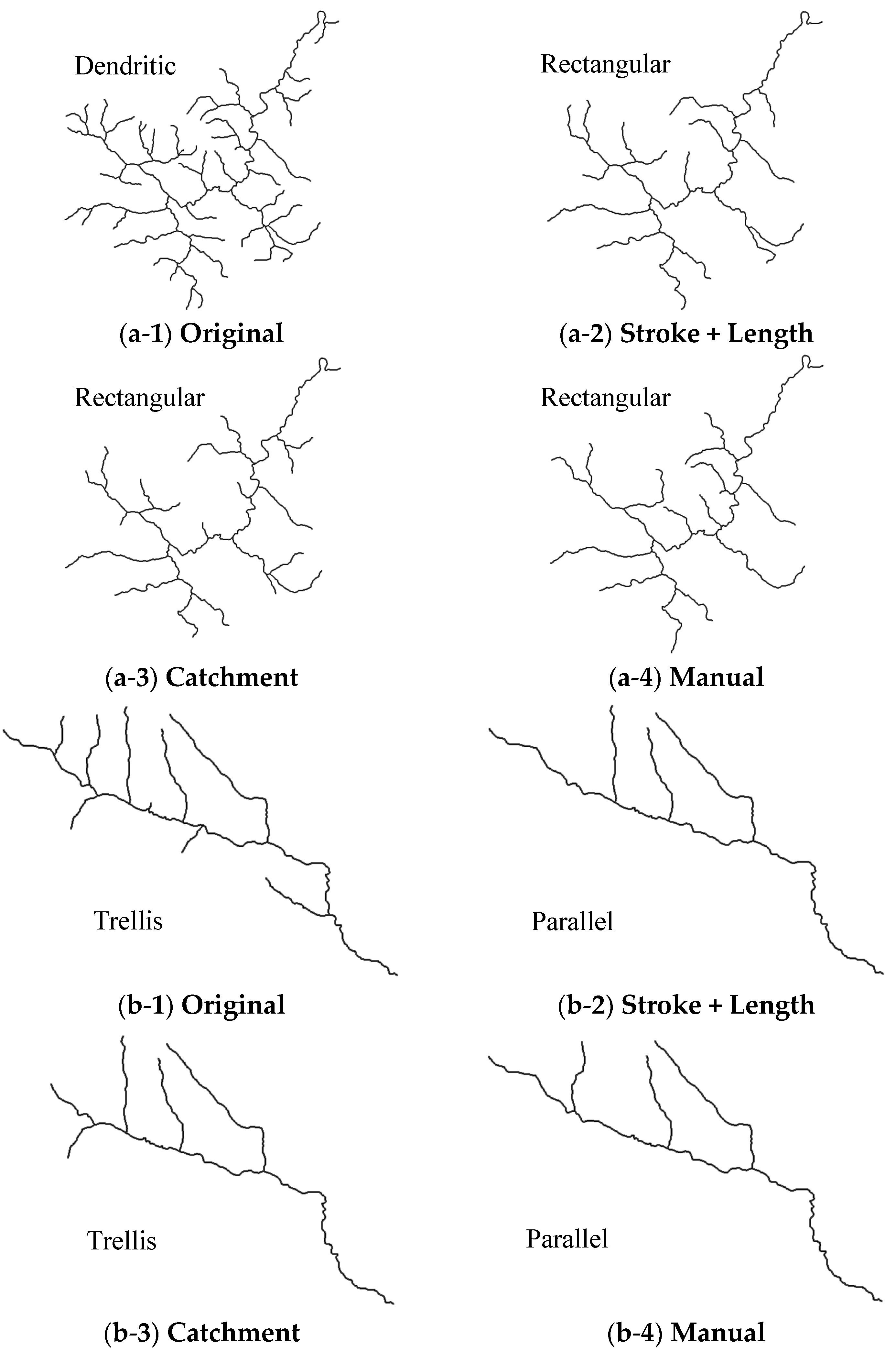
| (a-1) | 83.52° | 10% | 1.43 | 1.42 | 0.041 | 0 | 0 | 0.020 |
| (a-2) | 108.65° | 29% | 0.84 | 1.42 | 0 | 0 | 0.053 | 0.169 |
| (a-3) | 100.80° | 22% | 0.95 | 1.55 | 0 | 0 | 0.004 | 0.093 |
| (a-4) | 104.98° | 23% | 0.97 | 1.46 | 0 | 0 | 0.001 | 0.102 |
| (b-1) | 64.03° | 5% | 0.13 | 3.17 | 0 | 0 | 0.034 | 0.006 |
| (b-2) | 55.23° | 0 | 0.23 | 4.32 | 0 | 0.051 | 0.002 | 0 |
| (b-3) | 67.26° | 0 | 0.22 | 2.78 | 0.025 | 0 | 0.075 | 0 |
| (b-4) | 49.49° | 0 | 0.22 | 4.32 | 0 | 0.093 | 0 | 0 |
© 2016 by the authors; licensee MDPI, Basel, Switzerland. This article is an open access article distributed under the terms and conditions of the Creative Commons Attribution (CC-BY) license (http://creativecommons.org/licenses/by/4.0/).
Share and Cite
Zhang, L.; Guilbert, E. Evaluation of River Network Generalization Methods for Preserving the Drainage Pattern. ISPRS Int. J. Geo-Inf. 2016, 5, 230. https://doi.org/10.3390/ijgi5120230
Zhang L, Guilbert E. Evaluation of River Network Generalization Methods for Preserving the Drainage Pattern. ISPRS International Journal of Geo-Information. 2016; 5(12):230. https://doi.org/10.3390/ijgi5120230
Chicago/Turabian StyleZhang, Ling, and Eric Guilbert. 2016. "Evaluation of River Network Generalization Methods for Preserving the Drainage Pattern" ISPRS International Journal of Geo-Information 5, no. 12: 230. https://doi.org/10.3390/ijgi5120230