Spatial Sampling Strategies for the Effect of Interpolation Accuracy

Abstract

Spatial interpolation methods are widely used in various fields and have been studied by several scholars with one or a few specific sampling datasets that do not reflect the complexity of the spatial characteristics and lead to conclusions that cannot be widely applied. In this paper, three factors that affect the accuracy of interpolation have been considered, i.e., sampling density, sampling mode, and sampling location. We studied the inverse distance weighted (IDW), regular spline (RS), and ordinary kriging (OK) interpolation methods using 162 DEM datasets considering six sampling densities, nine terrain complexities, and three sampling modes. The experimental results show that, in selective sampling and combined sampling, the maximum absolute errors of interpolation methods rapidly increase and the estimated values are overestimated. In regular-grid sampling, the RS method has the highest interpolation accuracy, and IDW has the lowest interpolation accuracy. However, in both selective and combined sampling, the accuracy of the IDW method is significantly improved and the RS method performs worse. The OK method does not significantly change between the three sampling modes. The following conclusion can be obtained from the above analysis: the combined sampling mode is recommended for sampling, and more sampling points should be added in the ridges, valleys, and other complex terrain. The IDW method should not be used in the regular-grid sampling mode, but it has good performance in the selective sampling mode and combined sampling mode. However, the RS method shows the opposite phenomenon. The sampling dataset should be analyzed before using the OK method, which can select suitable models based on the analysis results of the sampling dataset.

1. Introduction

Spatial interpolation is the procedure of deriving the characteristic values of unknown data at specified points and the characteristics of data distribution based on the known data at specific points in the same area, which plays a significant role in spatial analysis [1].

More than twenty spatial interpolation methods have been used in different fields. According to the mathematical mechanism of interpolation, these interpolation methods can be classified as non-geostatistical methods and geostatistical methods. Non-geostatistical methods include the nearest neighbor method, inverse distance weighted method, local polynomial method, and regular spline method. The kriging method is the most common geostatistical method. Each interpolation method has different factors that affect the interpolation accuracy, and all affecting factors should be considered when interpolation methods are used. For example, the variance and variograms should be analyzed before using the kriging interpolation method.

Spatial interpolation methods have been applied in various fields. In the research of temperature interpolation, Wu et al. proposed a method for setting parameters and selecting models, in which the sampling points of observation stations were used and “one best method” was selected from several interpolation methods [2]. Phillips et al. selected the IDW and kriging methods for temperature simulation, and an optimal interpolation method was selected by comparing the absolute errors and root mean squared errors of IDW and kriging [3,4,5,6]. Wang et al. evaluated eight interpolation methods for research on heavy metals; the nearest neighbor interpolation method had the worst performance, and the multifractal kriging interpolation method had the best performance. However, different heavy metals had significantly different spatial characteristics, which affected the accuracy of the interpolation [7]. Li et al. proposed the fractal interpolation method when studying the distribution of copper. The fractal interpolation method was suitable when the sampling points were distributed unevenly and had significant correlation [8]. In terrain analysis, Liu et al. analyzed the spatial variability of elevation, and the results showed that the OK method was the best interpolation method [9]. Wang used the IDW, RS, TS, and kriging interpolation methods to analyze aerial survey points, and the TS interpolation method provided the best interpolation with the highest interpolation accuracy [10]. In studying soil nutrients, Chen et al. used three interpolation methods (i.e., kriging, spline, and IDW) for interpolation of N, P, K and PH sampling points, and the spline interpolation method performed the worst [11]. Liu et al. proposed a method that combined ensemble learning with ancillary environmental information for improved interpolation of soil properties because the ensemble learning model can describe more locally-detailed information and more accurate spatial patterns for soil potassium content than the other methods (i.e., kriging and IDW) [12].

From the above review, most scholars have studied interpolation methods by (1) comparing a few interpolation methods for a particular sampling dataset to determine the “best” interpolation method for a particular area of application, and (2) applying some assistant methods to improve one interpolation method for better accuracy. Both aspects can help obtain a good result for the specified sampling points. However, it is inappropriate to apply the conclusions to other sampling points because the sampling points used in a particular study may lack comprehensive representatives. In the case of terrain analysis, for example, a set of specified elevation sampling points can reflect only one region, which has a specific complexity, and the specified elevation sampling points differ from other sampling points with different sampling modes and sampling densities.

In this study, the influence of the terrain complexity, sampling mode, and sampling density on the accuracy of the interpolation results derived from different interpolation methods are investigated. The first section introduces the function, situation, problems, and the objective of this paper; the second section introduces the interpolation methods and the affecting factors selected in this paper; the third section gives the details of the experimental procedures; the fourth section provides the results of the experiment; the fifth section presents a discussion of the results; and the sixth chapter presents the conclusions of this study.

2. Spatial Interpolation Methods

Considering the variety and representativeness of interpolation methods, three interpolation methods are selected in this paper: two are classified as non-geostatistical methods (IDW and RS) and one is classified as a geostatistical method (OK). These three methods are commonly used and are representative of interpolation methods. The following provides a brief introduction to these methods.

(1) IDW: inverse distance weighting or weighted method is the simplest interpolation method and estimates the values at unsampled points using the distances to and values of nearby sampled points. IDW is based on the principle: closer things are similar. The principle assumes that two close sample points have similar attributes, and further sample points have less similar attributes. In this method, the value of a cell is the weighted average of the values of sample points nearby. A point closer to the cell in question carries a larger weight. IDW is a simple and effective interpolation method. The computation speed is relatively fast. In addition to the weighted distances, the power and search radius are also important factors affecting an IDW interpolation result [13]. The estimated values can be determined by the following equation:

$$\begin{array}{c}{Z}_0={\displaystyle \sum _{i=1}^n{\lambda }_i{Z}_i}\end{array}$$

(1)

where λ_i is the inverse distance weight, Z₀ is the predicted value, and Z_i is the measured value.

(2) RS: spline interpolation is based on the following principle: the interpolation interval is divided into small subintervals. Each of these subintervals is interpolated using the third-degree polynomial. The polynomial coefficients are chosen to satisfy certain conditions (these conditions depend on the interpolation method). General requirements are function continuity and passing through all given points. There are additional possible requirements: function linearity between nodes and continuity of higher derivatives. The main advantages of spline interpolation are its stability and calculation implicitly. Sets of linear equations, which are solved to construct splines, are well-conditioned; therefore, the polynomial coefficients are calculated precisely [14]. The equation of the regular spline interpolation is as follows:

$$\begin{array}{c}{Z}_0={\alpha }_1+{\alpha }_{2}x+{\alpha }_{3}y+{\displaystyle \sum _{j=1}^N{\lambda }_{j}R\left(r_j\right)}\end{array}$$

(2)

where α₁, α₂, α₃ are coefficients of the equations, N is the number of sampling points, λ_i is the weights, and R(r_j) is the spline function used to modify the interpolation results.

(3) OK: used in statistics, originally in geostatistics. Kriging is a method of interpolation for which the interpolated values are modeled by a Gaussian process governed by prior covariances, as opposed to a piecewise-polynomial spline chosen to optimize the smoothness of the fitted values. Under suitable assumptions of the priors, kriging gives the best linear, unbiased prediction of intermediate values.

Ordinary kriging is the most widely used kriging method. OK estimates a value at a point of a region for which a variogram is known using data in the neighborhood of the estimation location. OK assumes that the expected value of the interpolation field is an unknown constant [15]. The estimated values can be determined by the following equation:

$$Z_0=z(x_0)+{\displaystyle \sum _{i=1}^n\left(w_i\left(x_0\right)z\left(x_i\right)-z(x_0)\right)}$$

(3)

where Z₀ is the predicted value, z(x_i) is the measured value, w_i(x₀) is the weights reflecting the structural “proximity” of samples to the estimation location (x₀), and z(x₀) is the mathematical expectation of the sampling points.

The spatial characteristics of sampling points play a significant role in spatial interpolation and are determined by three factors: (1) where to sample; (2) what mode to sample (e.g., systematic or adaptive); and (3) how many points to sample (i.e., density). Samplings at different locations have different terrain situations, which represent different terrain complexities. The mode of sampling represents the way in which the sampling points are spatially distributed. For example, in the systematic (regular-grid) sampling mode, the sampling points are evenly distributed, whereas under the adaptive (selective) sampling mode, the sampling points are determined by the feature points of the terrain. The density of sampling points, i.e., the number of sampling points in a given region, has a significant effect on the interpolation accuracy. In this paper, the accuracy of the results generated by different spatial interpolation methods is studied with respect to datasets with different levels of terrain complexity, sampling density, and sampling modes.

3. Methods

3.1. Data Preparation and Processing

DEM data are widely used to describe surface topography. In this study, the DEM data are from the International Scientific Data Service Platform (http://www.cnic.cas.cn/) [16], and the resolution of the DEM data is 30 m × 30 m. A large amount of DEM data, covering more than 80% of China, has been collected and to reflect the comprehensive complexities of the terrain, a group of regions with different complexities, which are represented by fractal dimensions from 2.0 to 2.8, are chosen in this paper. We obtain the sampling points under different sampling modes and sampling densities, which have different spatial characteristics. The overall procedure and details are further described in Section 3.2.

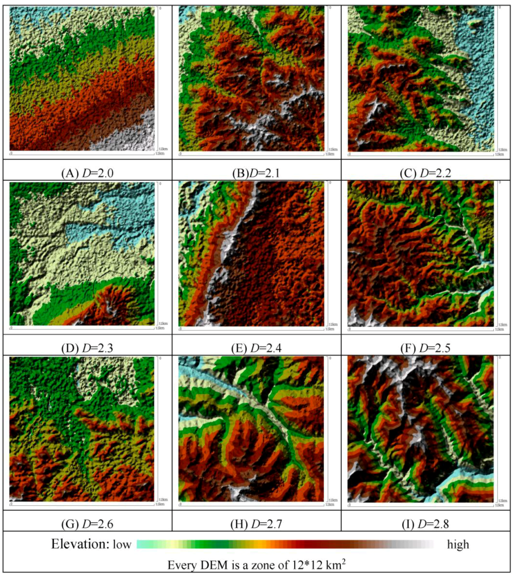
Fractal dimensions can be used to describe the variations of terrain in the entire study region and to indicate the level of terrain complexity, which includes the surface-volume method, the cubic covering method, and the surface-scale method. For the DEM data, surface or volume is calculated before obtaining the fractal dimension, which causes errors [17,18,19,20]. To decrease the errors, the cubic covering method is used in this paper. Some terrain data with different levels of terrain complexity D are shown in Figure 1.

Figure 1. Terrain data with different terrain complexity. (A) D = 2.0; (B) D = 2.1; (C) D = 2.2; (D) D = 2.3; (E) D = 2.4; (F) D = 2.5; (G) D = 2.6; (H) D = 2.7; (I) D = 2.8.

Figure 1. Terrain data with different terrain complexity. (A) D = 2.0; (B) D = 2.1; (C) D = 2.2; (D) D = 2.3; (E) D = 2.4; (F) D = 2.5; (G) D = 2.6; (H) D = 2.7; (I) D = 2.8.

Considering the national surveying specifications and characteristics of DEM, each DEM block is 144 km² (12 km × 12 km), and six sampling densities are used in this paper (i.e., 18.1 points/km², 5 points/km², 4.7 points/km², 3.1 points/km², 2.3 points/km², and 1.8 points/km²).

The sampling mode refers to the specific rules and methods used in determining the locations of the sampling points. Many sampling modes are adopted in interpolation research, and they can be divided into two large categories according to the distribution of sampling points: uniform sampling and non-uniform sampling. Some scholars used less popular methods, such as profile sampling and asymptotic sampling; OÈzdamar et al. applied herringbone-shaped, regular-grid, and layered random sampling modes in studying interpolation methods [21]. Demirhan et al. used four modes to sample the area under study: herringbone-shaped, regular-grid, linear, and ring sampling modes [22]. The sampling modes they used can be performed by computer but cannot accurately represent terrain feature points. To solve this problem, the regular-grid sampling mode, selective sampling mode, and combined sampling mode are used in this paper. The selective sampling mode focuses on terrain feature points when sampling, whereas the combined sampling mode takes the regular-grid sampling mode and selective sampling mode into consideration at the same time.

3.2. Experiment Design

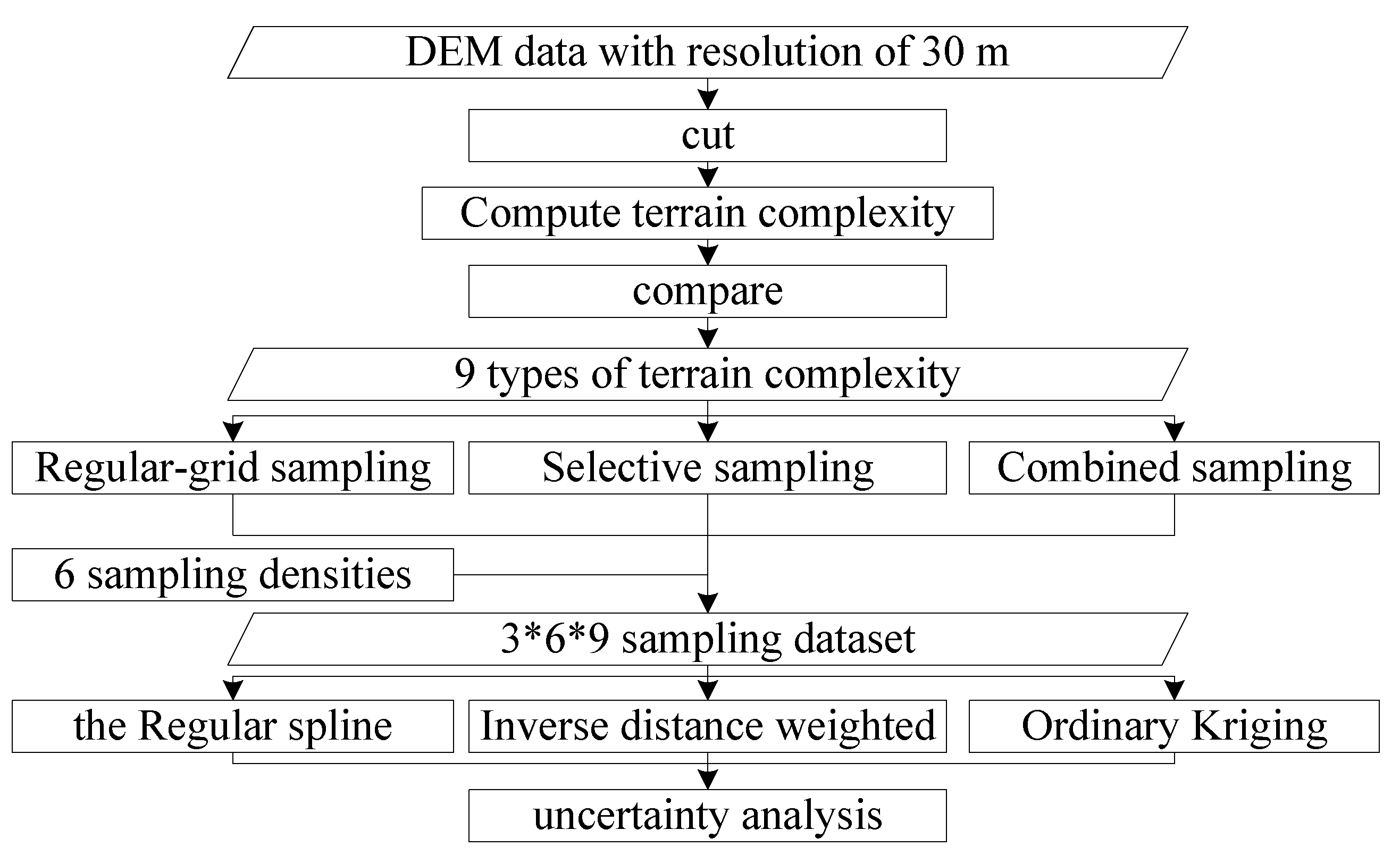
To systematically study how the spatial interpolation methods are affected by terrain complexity, sampling mode, and sampling density, DEM data with a resolution of 30 m are first divided into a series of data blocks with equal area. Next, data blocks with nine types of terrain complexity (sequentially increasing from level 2.0 to 2.8) are selected, and each block is sampled in three sampling modes and at six sampling densities for each mode. Finally, these point datasets are interpolated with different interpolation methods, and accuracy analysis is conducted. This procedure is illustrated in Figure 2.

Figure 2. Flow diagram of the experiment.

Figure 2. Flow diagram of the experiment.

3.3. Determination of Affecting Factors

The parameters of the interpolation methods have significant influences on the interpolation results, but there is no particular “best value” for the parameters. The parameters for IDW and RS in this paper are set using default values from ArcGIS 10.0, which are set by multiple tests. For OK, through repeated tests and validations, the spherical method is selected in this paper.

3.4. Validation

Independent verification is used for the validation of the interpolators in this paper. Each DEM is 12 km × 12 km and contains 400 × 400 sampling points. These sampling points are divided into the interpolation and validation subsets, estimating the value using interpolation subset and comparing the interpolated value at every validation point with its measured value. For the six levels of sampling density, 2704, 1225, 676, 441, 324, and 256 training points are created as interpolation data sets. The remaining, 157,269, 158,775, 159,559, 159,676, and 159,744 sampling points are used as validation datasets.

3.5. Assessment Indices

Many indices have been developed to assess the spatial interpolation accuracy. Each index alone cannot fully reflect the overall characteristics of the errors, so multiple indices are used in the analysis. In this paper, we use the three most common indices, i.e., maximum absolute errors (MAX), bias of errors (BIAS), and root mean squared of errors (RMSE), as measures of the interpolation accuracy. These three indices are determined by the following equations, where e₁, e₂, …, e_n are the errors between validation points and interpolation, abs(e₁), abs(e₂), …, abs(e_n) are the absolute values of e₁, e₂, …, e_n, and n is the number of validation points.

$$MAX=\max \left(\text{abs}\left(e_1\right),\text{abs}\left(e_2\right)\cdots \text{abs}\left(e_n\right)\right)$$

(4)

$$BIAS=\left(e_1+e_2+\cdots +e_n\right)/n$$

(5)

$$RMSE=\sqrt{\left(e_1^2+e_2^2+\cdots +e_n^2\right)/n}$$

(6)

4. Results

The accuracy of the interpolation results of the three methods is analyzed with respect to four characteristics: the distribution of errors, MAX, BIAS, and RMSE. The effects of the sampling mode, sampling density, and terrain complexity on interpolation results are also comprehensively analyzed and discussed, and the results are as follows.

4.1. Spatial Distribution of Errors

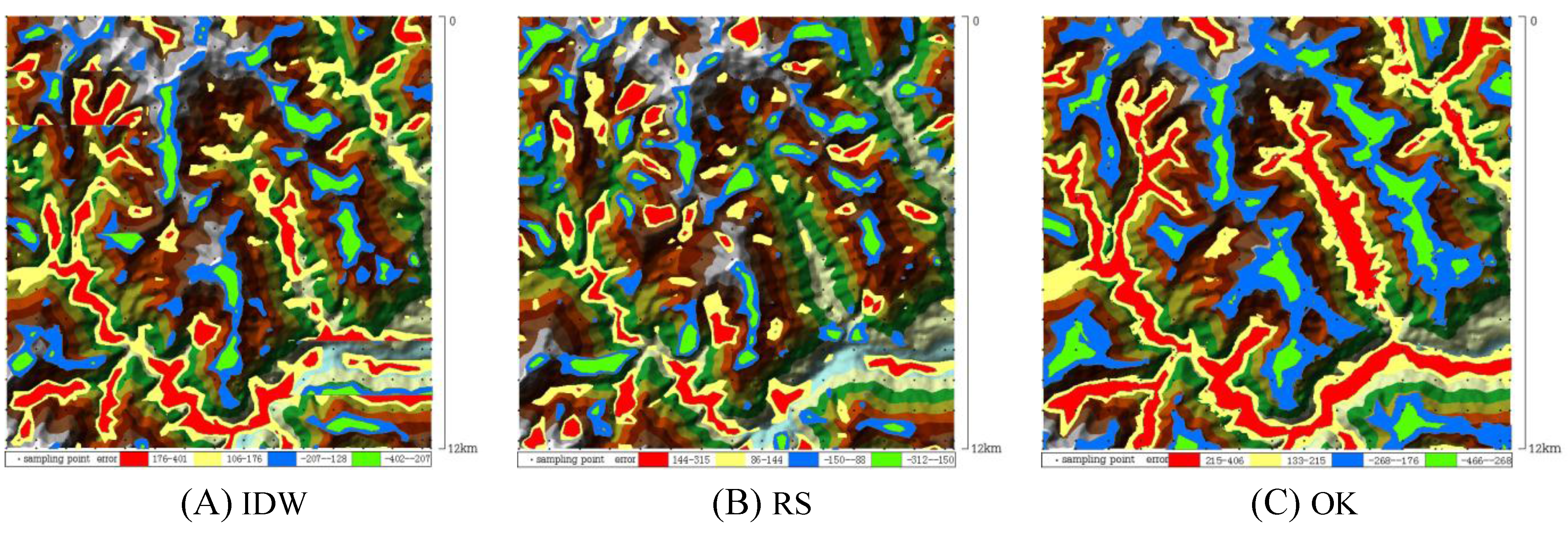
4.1.1. Regular-Grid Sampling

In regular-grid sampling, the distributions of errors of the three interpolation methods have the following characteristics (Figure 3):

The major locations of the error distribution are similar, in the mountain ridges, valleys, and peaks. With an increase of sampling density, the number of plaques of error-distributed area increases abruptly, and the size of the plaques gradually decreases. For the OK method, the distribution of errors follows the directions of the mountain ridges and valleys. At higher densities of sampling points, the error-distributed areas are mostly broken, and at lower densities of sampling points, the error-distributed areas are mostly continuous, with the least number of small error plaques. The size of the error-distributed areas is much larger than that of the other two methods.

Figure 3. The distributions of errors in regular-grid sampling. (A) Error distributions of IDW; (B) Error distributions of IDW; (C) Error distributions of IDW.

Figure 3. The distributions of errors in regular-grid sampling. (A) Error distributions of IDW; (B) Error distributions of IDW; (C) Error distributions of IDW.

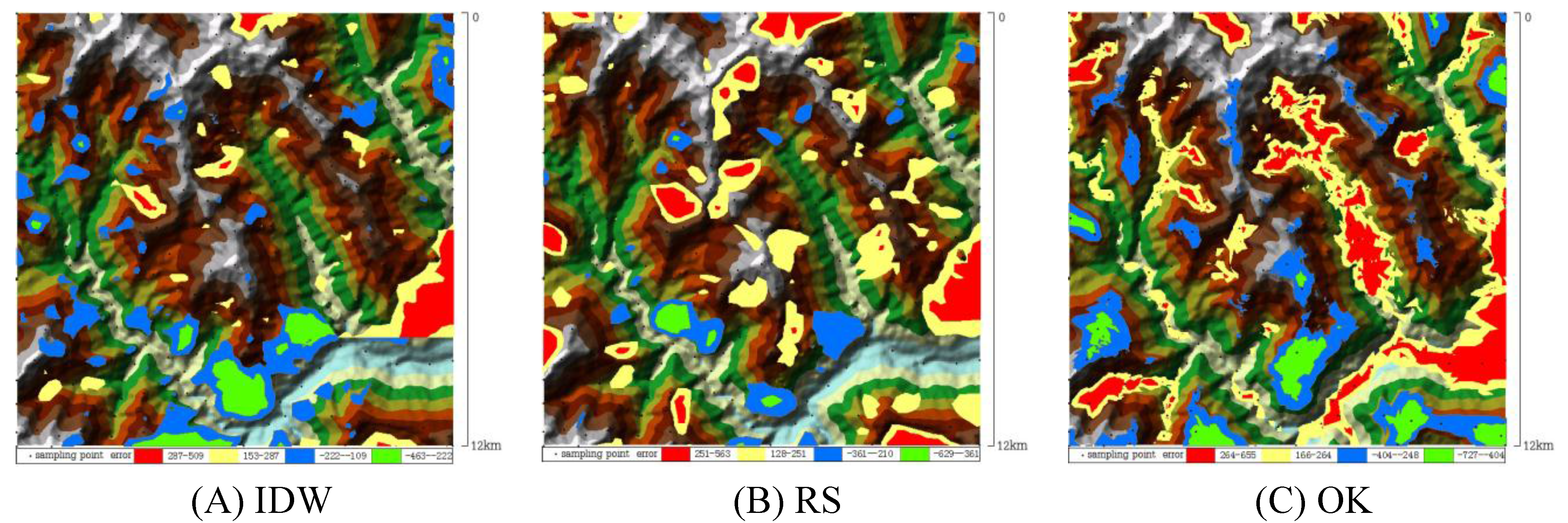
4.1.2. Selective Sampling

In selective sampling, the distributions of errors are different from those of regular-grid sampling, and the following characteristics are found (Figure 4):

The major locations of the error distribution are similar in the mountain ridges, valleys, and peaks. With an increase of sampling density, the number of plaques of error-distributed area increases abruptly, and the size of the plaques gradually decreases. In regions with sparsely distributed sampling points, large blocks of error-distributed area appear, and for the OK method, the distribution of errors follows the direction of mountain ridges and valleys. At high densities of sampling points, many small plaques of error-distributed area are found, and at low densities of sampling points, the least number of small plaques of error-distributed area are found. The error-distributed areas are much larger than those of the other two methods.

Figure 4. The distributions of errors in selective sampling. (A) Error distributions of IDW; (B) Error distributions of IDW; (C) Error distributions of IDW.

Figure 4. The distributions of errors in selective sampling. (A) Error distributions of IDW; (B) Error distributions of IDW; (C) Error distributions of IDW.

4.1.3. Combined Sampling

In the case of combined sampling, the following characteristics are found (Figure 5):

The major locations of the error distribution are similar in the mountain ridges, valleys, and peaks. For the OK method, the distribution of errors follows the direction of the mountain ridges and valleys. At high densities of sampling points, many small plaques of error-distributed area are found, and at low densities of sampling points, the least number of small plaques of error-distributed area are found. The error-distributed area is much larger than those of the other two methods.

Figure 5. The distributions of errors in combined sampling. (A) Error distributions of IDW; (B) Error distributions of IDW; (C) Error distributions of IDW.

Figure 5. The distributions of errors in combined sampling. (A) Error distributions of IDW; (B) Error distributions of IDW; (C) Error distributions of IDW.

4.1.4. Comprehensive analysis

In all sampling modes, the major locations of error distribution are in the mountain ridges, valleys, and peaks. In the selective sampling mode, large blocks of error-distributed area occur when the sampling points are sparse. With the increase of sampling density, the number of plaques of error-distributed area increases abruptly, and the size of the plaques gradually decreases.

The OK method has the maximum area of error distribution, with the most broken area at high sampling densities and the most continuous area and the least number of small error plaques at low sampling densities.

4.2. MAX

4.2.1. Regular-Grid Sampling

The experimental results show that the MAXes of the three methods have the following patterns in regular-grid sampling (Table 1):

With the increase of terrain complexity, the MAXes increase. With the increase of sampling density, MAXes decrease. With the decrease of sampling density, MAXes somewhat increase. The IDW method has the largest MAXes among the three methods, and the RS method has the smallest MAXes among the three methods.

4.2.2. Selective Sampling

In selective sampling, the experimental results show the following patterns (Table 2):

Table 1. The MAXs under the regular-grid sampling mode (Unit: m).

		Inverse Distance Weighted Method									Regular Spline Method									Ordinary Kriging Method
	D	2.0	2.1	2.2	2.3	2.4	2.5	2.6	2.7	2.8	2.0	2.1	2.2	2.3	2.4	2.5	2.6	2.7	2.8	2.0	2.1	2.2	2.3	2.4	2.5	2.6	2.7	2.8
SD
18.1		21	48	51	116	84	100	153	230	283	22	25	39	52	54	62	136	133	124	21	27	44	55	85	53	95	140	262
8.5		23	49	74	96	104	134	173	299	293	26	39	62	89	74	83	150	153	158	22	40	61	85	96	81	163	151	278
4.7		23	56	85	148	101	139	224	314	361	24	44	78	80	96	107	166	174	207	22	41	81	89	98	90	172	175	358
3.1		22	63	84	159	111	137	218	377	348	23	60	76	106	110	122	205	215	232	22	59	69	113	114	106	208	214	396
2.3		22	65	97	156	110	137	239	357	400	25	61	75	116	127	130	205	259	282	24	61	80	124	112	131	206	259	471
1.8		23	69	87	175	114	168	242	500	402	30	68	88	116	142	124	223	274	315	25	69	85	130	113	123	226	276	466

(D: Dimension of Terrain Complexity; SD: Sampling Density, Unit: Points/km²).

Table 1. The MAXs under the regular-grid sampling mode (Unit: m).

		Inverse Distance Weighted Method									Regular Spline Method									Ordinary Kriging Method
	D	2.0	2.1	2.2	2.3	2.4	2.5	2.6	2.7	2.8	2.0	2.1	2.2	2.3	2.4	2.5	2.6	2.7	2.8	2.0	2.1	2.2	2.3	2.4	2.5	2.6	2.7	2.8
SD
18.1		21	48	51	116	84	100	153	230	283	22	25	39	52	54	62	136	133	124	21	27	44	55	85	53	95	140	262
8.5		23	49	74	96	104	134	173	299	293	26	39	62	89	74	83	150	153	158	22	40	61	85	96	81	163	151	278
4.7		23	56	85	148	101	139	224	314	361	24	44	78	80	96	107	166	174	207	22	41	81	89	98	90	172	175	358
3.1		22	63	84	159	111	137	218	377	348	23	60	76	106	110	122	205	215	232	22	59	69	113	114	106	208	214	396
2.3		22	65	97	156	110	137	239	357	400	25	61	75	116	127	130	205	259	282	24	61	80	124	112	131	206	259	471
1.8		23	69	87	175	114	168	242	500	402	30	68	88	116	142	124	223	274	315	25	69	85	130	113	123	226	276	466

(D: Dimension of Terrain Complexity; SD: Sampling Density, Unit: Points/km²).

Table 2. The MAXs under selective sampling mode (Unit: m).

		Inverse Distance Weighted Method									Regular Spline Method									Ordinary Kriging Method
	D	2.0	2.1	2.2	2.3	2.4	2.5	2.6	2.7	2.8	2.0	2.1	2.2	2.3	2.4	2.5	2.6	2.7	2.8	2.0	2.1	2.2	2.3	2.4	2.5	2.6	2.7	2.8
SD
18.1		23	60	72	86	89	111	214	405	376	35	41	46	49	144	120	130	174	210	20	31	35	39	88	81	114	212	265
8.5		28	51	79	113	82	114	194	459	305	57	68	64	75	94	134	160	267	329	23	31	45	41	94	80	121	187	354
4.7		22	45	92	123	120	126	146	325	350	33	80	99	75	125	348	192	331	321	24	51	63	61	102	90	112	234	306
3.1		25	56	78	113	98	175	139	363	350	44	108	94	84	250	159	266	479	336	23	59	64	72	103	91	146	212	353
2.3		31	53	89	119	87	198	211	352	465	43	127	98	86	167	181	343	562	490	28	60	77	57	104	115	155	345	460
1.8		31	49	65	159	100	160	188	334	509	49	98	111	168	278	309	280	426	629	27	51	68	72	111	196	166	335	727

Table 2. The MAXs under selective sampling mode (Unit: m).

		Inverse Distance Weighted Method									Regular Spline Method									Ordinary Kriging Method
	D	2.0	2.1	2.2	2.3	2.4	2.5	2.6	2.7	2.8	2.0	2.1	2.2	2.3	2.4	2.5	2.6	2.7	2.8	2.0	2.1	2.2	2.3	2.4	2.5	2.6	2.7	2.8
SD
18.1		23	60	72	86	89	111	214	405	376	35	41	46	49	144	120	130	174	210	20	31	35	39	88	81	114	212	265
8.5		28	51	79	113	82	114	194	459	305	57	68	64	75	94	134	160	267	329	23	31	45	41	94	80	121	187	354
4.7		22	45	92	123	120	126	146	325	350	33	80	99	75	125	348	192	331	321	24	51	63	61	102	90	112	234	306
3.1		25	56	78	113	98	175	139	363	350	44	108	94	84	250	159	266	479	336	23	59	64	72	103	91	146	212	353
2.3		31	53	89	119	87	198	211	352	465	43	127	98	86	167	181	343	562	490	28	60	77	57	104	115	155	345	460
1.8		31	49	65	159	100	160	188	334	509	49	98	111	168	278	309	280	426	629	27	51	68	72	111	196	166	335	727

With the increase of terrain complexity, the MAXes increase significantly. With the increase of sampling density, the MAXes somewhat decrease. With the decrease of sampling density, the MAXes increase, and a greater increase is found at lower sampling density. The OK method has the minimum MAXes among the three methods, and for the other two methods, the RS method has smaller MAXes at higher sampling density and the IDW method has smaller MAXes at lower sampling density.

4.2.3. Combined Sampling

In combined sampling, the experimental results show the following patterns (Table 3):

With the increase of terrain complexity, the MAXes also increase. With the increase of sampling density, the MAXes somewhat decrease. With the decrease of sampling density, a greater increase is found at lower sampling density. The OK method has the smallest MAXes among the three methods, and for the other two methods, the RS method has smaller MAXes at higher sampling density and the IDW method has smaller MAXes at lower sampling density.

4.2.4. Comprehensive Analysis

Statistical analysis of the MAXes for all sampling modes, nine sampling densities, and six levels of terrain complexity found the following results.

In all sampling modes, with the increase of terrain complexity, the MAXes also increase. With the increase of sampling density, the MAXes decrease relatively and vice versa. In regular-grid sampling, for all sampling densities and levels of terrain complexity, the RS method has the minimum MAXes among the three methods. In selective sampling and combined sampling, the OK method has the minimum MAXes among the three methods.

4.3. BIAS

4.3.1. Regular-Grid Sampling

For regular-grid sampling, the BIASes of the three methods are shown in Table 4, which shows the following characteristics:

With the increase of terrain complexity, the BIASes of all methods also increase. With the decrease of the sampling density, the BIASes of all methods increase, and vice versa. BIASes are not noticeably overestimated or underestimated. The RS method has the minimum BIASes among the three methods, and the IDW method has the maximum BIASes among the three methods.

Table 3. The MAXs under combined sampling mode (Unit: m).

		Inverse Distance Weighted Method									Regular Spline Method									Ordinary Kriging Method
	D	2.0	2.1	2.2	2.3	2.4	2.5	2.6	2.7	2.8	2.0	2.1	2.2	2.3	2.4	2.5	2.6	2.7	2.8	2.0	2.1	2.2	2.3	2.4	2.5	2.6	2.7	2.8
SD
18.1		20	48	58	117	84	99	153	253	290	25	24	39	55	53	62	132	133	127	17	22	43	48	84	53	96	140	296
8.5		22	50	74	95	98	133	148	230	290	27	45	61	78	93	101	117	157	228	23	40	58	58	93	80	99	143	308
4.7		28	48	65	148	100	130	224	300	357	27	51	70	89	148	121	192	199	222	23	44	55	74	83	78	157	177	362
3.1		22	50	72	126	128	155	215	340	374	31	59	82	148	176	127	217	242	409	24	40	70	99	98	85	144	225	419
2.3		32	51	87	139	118	161	248	386	387	30	65	95	130	145	147	215	267	390	27	46	82	91	113	104	124	245	541
1.8		31	53	92	79	124	108	243	315	396	29	83	110	181	175	176	211	403	353	26	58	81	95	122	120	226	322	487

Table 3. The MAXs under combined sampling mode (Unit: m).

		Inverse Distance Weighted Method									Regular Spline Method									Ordinary Kriging Method
	D	2.0	2.1	2.2	2.3	2.4	2.5	2.6	2.7	2.8	2.0	2.1	2.2	2.3	2.4	2.5	2.6	2.7	2.8	2.0	2.1	2.2	2.3	2.4	2.5	2.6	2.7	2.8
SD
18.1		20	48	58	117	84	99	153	253	290	25	24	39	55	53	62	132	133	127	17	22	43	48	84	53	96	140	296
8.5		22	50	74	95	98	133	148	230	290	27	45	61	78	93	101	117	157	228	23	40	58	58	93	80	99	143	308
4.7		28	48	65	148	100	130	224	300	357	27	51	70	89	148	121	192	199	222	23	44	55	74	83	78	157	177	362
3.1		22	50	72	126	128	155	215	340	374	31	59	82	148	176	127	217	242	409	24	40	70	99	98	85	144	225	419
2.3		32	51	87	139	118	161	248	386	387	30	65	95	130	145	147	215	267	390	27	46	82	91	113	104	124	245	541
1.8		31	53	92	79	124	108	243	315	396	29	83	110	181	175	176	211	403	353	26	58	81	95	122	120	226	322	487

Table 4. The BIASs under regular-grid sampling mode (Unit: m).

		Inverse Distance Weighted Method									Regular Spline Method									Ordinary Kriging Method
	D	2.0	2.1	2.2	2.3	2.4	2.5	2.6	2.7	2.8	2.0	2.1	2.2	2.3	2.4	2.5	2.6	2.7	2.8	2.0	2.1	2.2	2.3	2.4	2.5	2.6	2.7	2.8
SD
18.1		−0.11	0.00	−0.15	−0.31	0.02	0.63	−0.14	0.56	1.19	−0.03	−0.01	−0.06	−0.03	0.02	−0.10	−0.14	−0.08	−0.06	−0.03	−0.02	−0.06	−0.05	0.00	−0.07	−0.17	−0.08	−0.21
8.5		0.19	−0.01	−0.05	−0.15	0.37	1.45	0.12	1.43	0.48	0.10	−0.01	−0.08	0.01	0.20	0.36	−0.35	−0.00	−0.05	0.09	−0.02	−0.09	0.00	0.22	0.27	−0.30	0.18	0.06
4.7		−0.08	0.13	0.06	−0.37	0.08	−0.73	−0.03	3.15	−2.19	−0.01	0.15	0.11	−0.12	−0.27	−1.02	−0.17	−0.18	0.12	−0.02	0.09	0.16	−0.06	−0.24	−0.97	−0.09	−0.05	−0.38
3.1		−0.02	0.00	0.42	−0.01	−0.70	1.04	1.40	−2.71	−2.09	0.10	0.28	0.16	−0.30	−0.03	0.07	1.17	−2.43	−1.35	0.07	0.18	0.18	−0.22	−0.36	−0.16	1.60	−2.00	−1.87
2.3		0.32	0.66	0.46	−0.04	0.10	1.54	−0.10	8.36	−1.89	0.097	0.620	−0.20	0.000	−0.81	0.224	−0.79	3.396	−1.01	0.06	0.57	−0.20	0.04	−0.93	−0.05	−0.51	3.31	1.03
1.8		0.17	0.04	1.66	−0.23	1.13	1.63	0.25	7.38	6.37	0.002	0.185	1.476	−0.05	0.49	0.255	−0.24	3.31	1.09	−0.01	0.07	1.58	0.09	0.37	0.22	0.05	2.74	4.59

Table 4. The BIASs under regular-grid sampling mode (Unit: m).

		Inverse Distance Weighted Method									Regular Spline Method									Ordinary Kriging Method
	D	2.0	2.1	2.2	2.3	2.4	2.5	2.6	2.7	2.8	2.0	2.1	2.2	2.3	2.4	2.5	2.6	2.7	2.8	2.0	2.1	2.2	2.3	2.4	2.5	2.6	2.7	2.8
SD
18.1		−0.11	0.00	−0.15	−0.31	0.02	0.63	−0.14	0.56	1.19	−0.03	−0.01	−0.06	−0.03	0.02	−0.10	−0.14	−0.08	−0.06	−0.03	−0.02	−0.06	−0.05	0.00	−0.07	−0.17	−0.08	−0.21
8.5		0.19	−0.01	−0.05	−0.15	0.37	1.45	0.12	1.43	0.48	0.10	−0.01	−0.08	0.01	0.20	0.36	−0.35	−0.00	−0.05	0.09	−0.02	−0.09	0.00	0.22	0.27	−0.30	0.18	0.06
4.7		−0.08	0.13	0.06	−0.37	0.08	−0.73	−0.03	3.15	−2.19	−0.01	0.15	0.11	−0.12	−0.27	−1.02	−0.17	−0.18	0.12	−0.02	0.09	0.16	−0.06	−0.24	−0.97	−0.09	−0.05	−0.38
3.1		−0.02	0.00	0.42	−0.01	−0.70	1.04	1.40	−2.71	−2.09	0.10	0.28	0.16	−0.30	−0.03	0.07	1.17	−2.43	−1.35	0.07	0.18	0.18	−0.22	−0.36	−0.16	1.60	−2.00	−1.87
2.3		0.32	0.66	0.46	−0.04	0.10	1.54	−0.10	8.36	−1.89	0.097	0.620	−0.20	0.000	−0.81	0.224	−0.79	3.396	−1.01	0.06	0.57	−0.20	0.04	−0.93	−0.05	−0.51	3.31	1.03
1.8		0.17	0.04	1.66	−0.23	1.13	1.63	0.25	7.38	6.37	0.002	0.185	1.476	−0.05	0.49	0.255	−0.24	3.31	1.09	−0.01	0.07	1.58	0.09	0.37	0.22	0.05	2.74	4.59

4.3.2. Selective Sampling

For selective sampling, the BIASes of the three methods are shown in Table 5, which shows the following patterns.

With the increase of terrain complexity, the BIASes of all methods also increase, but with a lower level of increase. With the decrease of the sampling density, the BIASes of all methods increase, and vice versa. Some BIASes are over-estimated. The IDW method has the maximum BIASes among the three methods, and the RS method has the minimum BIASes among the three methods.

4.3.3. Combined Sampling

For combined sampling, the BIASes of the three methods are shown in Table 6, which shows the following patterns.

With the increase of terrain complexity, the BIASes also increase, but the level of increase is lower than that of the other modes. With the decrease of the sampling density, BIASes slightly increase, and vice versa. Some BIASes are over-estimated. The IDW method has the maximum BIASes among the three methods, and the RS method has the minimum BIASes among the three methods.

4.3.4. Comprehensive Analysis

The statistical analysis of the errors for all sampling modes, nine sampling densities, and six levels of terrain complexity shows that the RS method has the minimum and the IDW method has the maximum BIASes in all cases.

4.4. RMSE

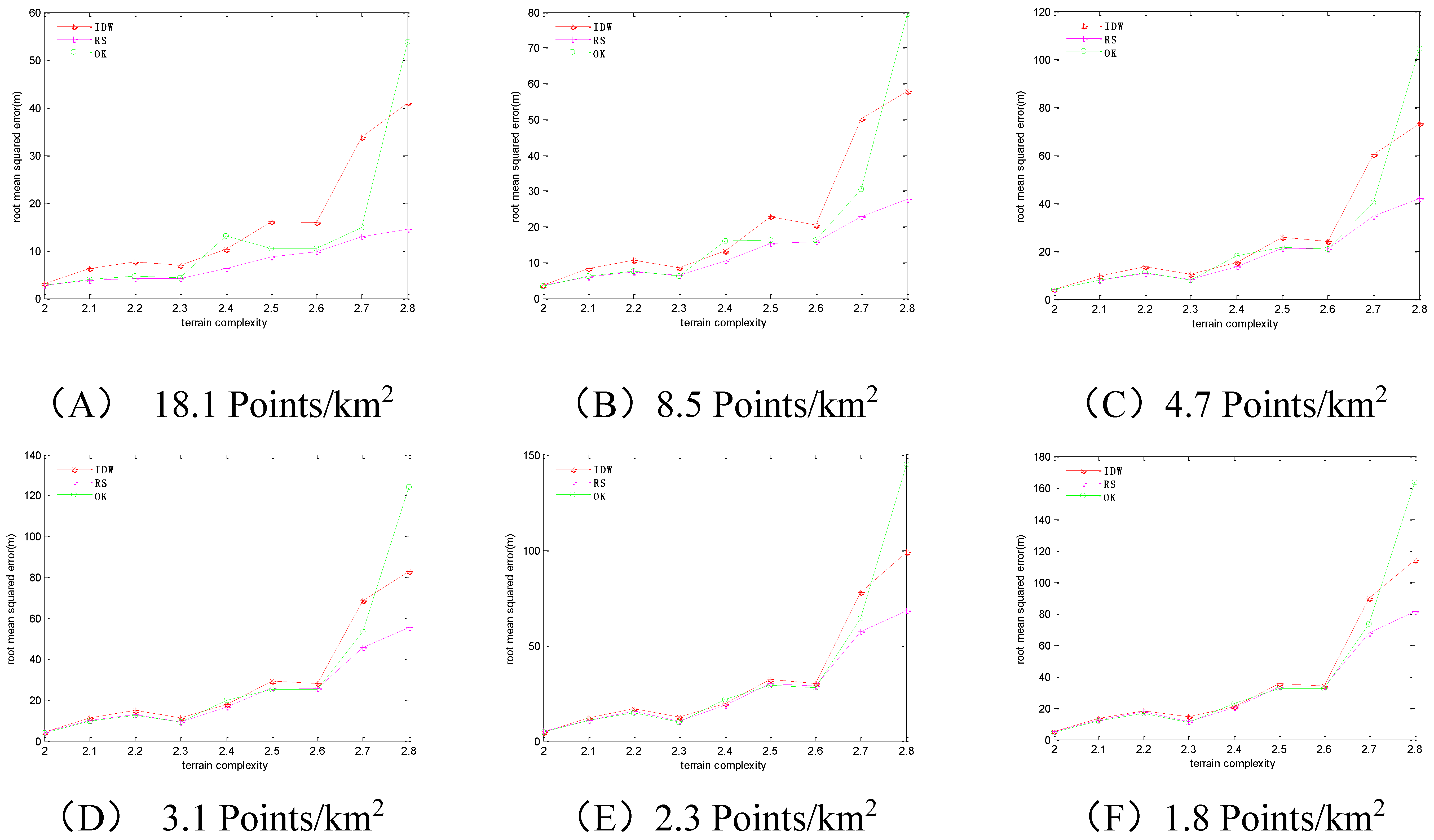
4.4.1. Regular-grid Sampling

For regular-grid sampling, the RMSEs of the three methods are shown in Figure 6 and Table 7, which have the following patterns.

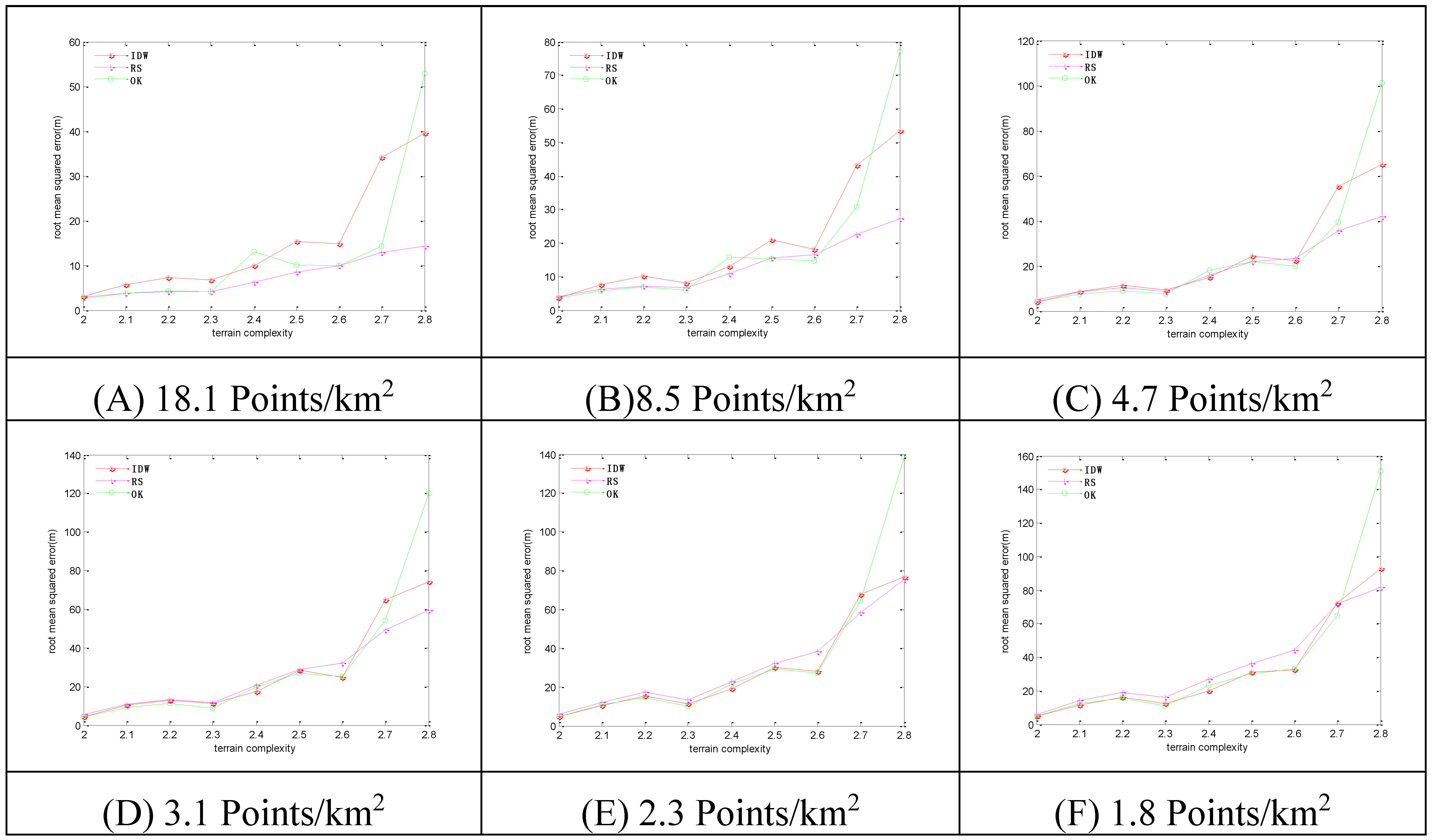
With the increase of terrain complexity, the RMSEs steeply increase. With the increase of sampling density, the RMSEs steadily decrease. The IDW method has the maximum RMSEs among the three methods, and the RS method has the minimum RMSEs among the three methods.

4.4.2. Selective Sampling

For selective sampling, the RMSEs of the three methods are shown in Figure 7 and Table 8, which have the following patterns:

With the increase of terrain complexity, the RMSEs steeply increase. With the increase of sampling density, the RMSEs decrease, and vice versa. For lower levels of terrain complexity, the OK method has the minimum RMSEs at high sampling density, and the IDW method has the minimum RMSEs at low sampling density. For higher levels of terrain complexity, the RS method has the minimum RMSEs at high sampling density, and the IDW method has the minimum RMSEs at low sampling density.

Table 5. The BIASs under selective sampling mode (Unit: m).

		Inverse Distance Weighted Method									Regular Spline Method									Ordinary Kriging Method
	D	2.0	2.1	2.2	2.3	2.4	2.5	2.6	2.7	2.8	2.0	2.1	2.2	2.3	2.4	2.5	2.6	2.7	2.8	2.0	2.1	2.2	2.3	2.4	2.5	2.6	2.7	2.8
SD
18.1		−0.02	0.85	1.49	0.66	1.25	1.42	2.22	5.89	0.31	−0.01	0.27	0.18	0.19	0.16	−0.19	0.28	−0.08	1.05	−0.04	0.31	0.38	0.18	1.30	1.19	0.66	0.75	0.70
8.5		0.78	3.10	4.72	1.55	2.22	0.79	6.40	6.75	3.17	1.09	1.01	1.34	0.82	2.35	1.44	6.49	0.65	2.83	0.87	1.93	2.92	0.80	1.85	1.42	6.12	1.84	1.88
4.7		0.83	2.79	7.22	3.40	5.88	5.88	6.49	1.20	13.39	1.01	1.72	3.17	2.14	6.49	5.73	3.41	0.26	5.79	0.92	2.25	3.93	2.56	5.64	5.15	4.60	−1.29	12.76
3.1		0.71	4.86	9.66	6.24	9.06	5.00	20.34	15.26	3.70	1.08	4.22	5.00	3.59	8.87	1.51	14.73	6.91	4.45	0.90	4.51	7.76	4.56	9.21	3.09	18.22	9.36	2.59
2.3		1.24	6.40	14.47	7.50	10.15	10.96	20.86	15.97	−2.78	1.64	5.61	7.14	4.83	9.22	11.07	17.52	−5.89	5.11	1.44	5.77	12.66	4.99	9.10	10.38	21.63	9.75	−1.58
1.8		0.69	6.90	13.04	8.21	13.47	5.83	27.41	18.82	5.64	1.31	3.61	7.16	4.33	9.68	4.49	24.81	1.27	10.93	1.10	5.32	11.43	4.68	12.75	5.66	27.08	14.62	−6.71

Table 5. The BIASs under selective sampling mode (Unit: m).

		Inverse Distance Weighted Method									Regular Spline Method									Ordinary Kriging Method
	D	2.0	2.1	2.2	2.3	2.4	2.5	2.6	2.7	2.8	2.0	2.1	2.2	2.3	2.4	2.5	2.6	2.7	2.8	2.0	2.1	2.2	2.3	2.4	2.5	2.6	2.7	2.8
SD
18.1		−0.02	0.85	1.49	0.66	1.25	1.42	2.22	5.89	0.31	−0.01	0.27	0.18	0.19	0.16	−0.19	0.28	−0.08	1.05	−0.04	0.31	0.38	0.18	1.30	1.19	0.66	0.75	0.70
8.5		0.78	3.10	4.72	1.55	2.22	0.79	6.40	6.75	3.17	1.09	1.01	1.34	0.82	2.35	1.44	6.49	0.65	2.83	0.87	1.93	2.92	0.80	1.85	1.42	6.12	1.84	1.88
4.7		0.83	2.79	7.22	3.40	5.88	5.88	6.49	1.20	13.39	1.01	1.72	3.17	2.14	6.49	5.73	3.41	0.26	5.79	0.92	2.25	3.93	2.56	5.64	5.15	4.60	−1.29	12.76
3.1		0.71	4.86	9.66	6.24	9.06	5.00	20.34	15.26	3.70	1.08	4.22	5.00	3.59	8.87	1.51	14.73	6.91	4.45	0.90	4.51	7.76	4.56	9.21	3.09	18.22	9.36	2.59
2.3		1.24	6.40	14.47	7.50	10.15	10.96	20.86	15.97	−2.78	1.64	5.61	7.14	4.83	9.22	11.07	17.52	−5.89	5.11	1.44	5.77	12.66	4.99	9.10	10.38	21.63	9.75	−1.58
1.8		0.69	6.90	13.04	8.21	13.47	5.83	27.41	18.82	5.64	1.31	3.61	7.16	4.33	9.68	4.49	24.81	1.27	10.93	1.10	5.32	11.43	4.68	12.75	5.66	27.08	14.62	−6.71

Table 6. The BIASs under combined sampling mode (Unit: m).

		Inverse Distance Weighted Method									Regular Spline Method									Ordinary Kriging Method
	D	2.0	2.1	2.2	2.3	2.4	2.5	2.6	2.7	2.8	2.0	2.1	2.2	2.3	2.4	2.5	2.6	2.7	2.8	2.0	2.1	2.2	2.3	2.4	2.5	2.6	2.7	2.8
SD
18.1		−0.03	0.17	0.20	−0.22	0.32	−0.11	−0.26	1.06	1.10	0.01	0.11	0.12	0.03	0.10	−0.11	−0.04	−0.10	0.07	0.00	0.09	0.08	0.02	0.18	−0.15	−0.12	−0.01	0.17
8.5		0.25	0.45	0.42	0.11	1.09	1.73	1.23	2.66	2.03	0.16	0.42	0.38	0.13	0.59	0.16	0.97	−0.29	0.67	0.15	0.39	0.32	0.13	0.80	0.06	0.91	0.38	−0.36
4.7		0.02	1.57	2.12	0.38	0.85	−0.70	0.92	2.71	−0.17	0.13	1.22	1.30	0.41	1.23	−1.69	1.15	1.35	0.47	0.12	1.22	1.46	0.50	0.71	−1.20	1.19	1.06	−0.45
3.1		0.22	1.99	2.70	0.64	2.85	−0.40	3.74	−0.49	0.62	0.19	2.35	2.41	0.25	2.69	−0.85	3.09	1.99	3.66	0.19	2.14	2.27	0.45	2.49	−0.92	3.63	0.83	−0.18
2.3		0.39	3.47	4.45	2.15	2.91	−1.12	5.86	7.83	3.90	0.12	2.66	2.72	0.87	1.55	−2.44	4.81	2.99	3.41	0.19	2.79	3.06	1.32	2.48	−2.42	5.44	3.28	4.06
1.8		0.44	4.50	6.34	3.63	4.49	−2.10	7.54	8.90	4.77	0.32	3.16	4.31	1.87	3.32	−1.11	4.35	4.03	3.58	0.28	3.84	5.27	2.48	4.06	−2.71	6.58	6.41	2.94

Table 6. The BIASs under combined sampling mode (Unit: m).

		Inverse Distance Weighted Method									Regular Spline Method									Ordinary Kriging Method
	D	2.0	2.1	2.2	2.3	2.4	2.5	2.6	2.7	2.8	2.0	2.1	2.2	2.3	2.4	2.5	2.6	2.7	2.8	2.0	2.1	2.2	2.3	2.4	2.5	2.6	2.7	2.8
SD
18.1		−0.03	0.17	0.20	−0.22	0.32	−0.11	−0.26	1.06	1.10	0.01	0.11	0.12	0.03	0.10	−0.11	−0.04	−0.10	0.07	0.00	0.09	0.08	0.02	0.18	−0.15	−0.12	−0.01	0.17
8.5		0.25	0.45	0.42	0.11	1.09	1.73	1.23	2.66	2.03	0.16	0.42	0.38	0.13	0.59	0.16	0.97	−0.29	0.67	0.15	0.39	0.32	0.13	0.80	0.06	0.91	0.38	−0.36
4.7		0.02	1.57	2.12	0.38	0.85	−0.70	0.92	2.71	−0.17	0.13	1.22	1.30	0.41	1.23	−1.69	1.15	1.35	0.47	0.12	1.22	1.46	0.50	0.71	−1.20	1.19	1.06	−0.45
3.1		0.22	1.99	2.70	0.64	2.85	−0.40	3.74	−0.49	0.62	0.19	2.35	2.41	0.25	2.69	−0.85	3.09	1.99	3.66	0.19	2.14	2.27	0.45	2.49	−0.92	3.63	0.83	−0.18
2.3		0.39	3.47	4.45	2.15	2.91	−1.12	5.86	7.83	3.90	0.12	2.66	2.72	0.87	1.55	−2.44	4.81	2.99	3.41	0.19	2.79	3.06	1.32	2.48	−2.42	5.44	3.28	4.06
1.8		0.44	4.50	6.34	3.63	4.49	−2.10	7.54	8.90	4.77	0.32	3.16	4.31	1.87	3.32	−1.11	4.35	4.03	3.58	0.28	3.84	5.27	2.48	4.06	−2.71	6.58	6.41	2.94

Figure 6. The RMSEs of the 3 methods in regular-grid sampling. Sampling densities of (A) 18.1 points/km²; (B) 8.5 points/km²; (C) 4.7 points/km²; (D) 3.1 points/km²; (E) 2.3 points/km²; (F) 1.8 points/km².

Figure 6. The RMSEs of the 3 methods in regular-grid sampling. Sampling densities of (A) 18.1 points/km²; (B) 8.5 points/km²; (C) 4.7 points/km²; (D) 3.1 points/km²; (E) 2.3 points/km²; (F) 1.8 points/km².

Table 7. The RMSEs under regular-grid sampling mode (Unit: m).

		Inverse Distance Weighted Method									Regular Spline Method									Ordinary Kriging Method
	D	2.0	2.1	2.2	2.3	2.4	2.5	2.6	2.7	2.8	2.0	2.1	2.2	2.3	2.4	2.5	2.6	2.7	2.8	2.0	2.1	2.2	2.3	2.4	2.5	2.6	2.7	2.8
SD
18.1		3.0	6.2	7.7	7.0	10.2	16.1	15.8	33.8	40.9	2.7	3.7	4.1	4.2	6.2	8.7	9.8	12.8	14.5	2.6	4.0	4.6	4.3	13.1	10.5	10.5	14.8	53.8
8.5		3.7	8.2	10.8	8.5	13.3	22.7	20.4	50.2	57.9	3.6	6.0	7.3	6.4	10.4	15.4	15.7	22.7	27.6	3.4	6.1	7.6	6.3	16.0	16.2	16.2	30.5	79.4
4.7		4.1	9.5	13.6	10.3	15.4	25.9	23.9	60.2	73.0	4.2	7.7	10.7	8.1	13.7	21.3	21.0	34.6	41.8	3.9	7.9	10.9	8.0	18.0	21.4	20.9	40.2	104.4
3.1		4.3	11.3	14.9	11.4	17.8	29.4	28.2	68.6	82.9	4.3	9.9	12.7	9.3	16.6	25.8	25.8	45.6	55.3	4.1	9.8	12.7	9.1	20.0	25.2	25.2	53.2	124.2
2.3		4.7	12.1	17.0	12.5	19.6	32.3	30.3	77.8	99.0	4.8	10.7	15.6	10.2	18.6	30.1	28.5	57.1	68.4	4.5	10.7	14.9	9.9	21.7	29.3	28.0	64.4	145.0
1.8		4.9	13.2	18.3	14.3	20.7	35.5	33.9	89.8	114.2	4.9	12.2	17.9	11.3	20.2	33.5	33.6	67.9	81.1	4.5	11.8	16.4	10.9	22.9	32.5	32.2	73.3	163.2

Table 7. The RMSEs under regular-grid sampling mode (Unit: m).

		Inverse Distance Weighted Method									Regular Spline Method									Ordinary Kriging Method
	D	2.0	2.1	2.2	2.3	2.4	2.5	2.6	2.7	2.8	2.0	2.1	2.2	2.3	2.4	2.5	2.6	2.7	2.8	2.0	2.1	2.2	2.3	2.4	2.5	2.6	2.7	2.8
SD
18.1		3.0	6.2	7.7	7.0	10.2	16.1	15.8	33.8	40.9	2.7	3.7	4.1	4.2	6.2	8.7	9.8	12.8	14.5	2.6	4.0	4.6	4.3	13.1	10.5	10.5	14.8	53.8
8.5		3.7	8.2	10.8	8.5	13.3	22.7	20.4	50.2	57.9	3.6	6.0	7.3	6.4	10.4	15.4	15.7	22.7	27.6	3.4	6.1	7.6	6.3	16.0	16.2	16.2	30.5	79.4
4.7		4.1	9.5	13.6	10.3	15.4	25.9	23.9	60.2	73.0	4.2	7.7	10.7	8.1	13.7	21.3	21.0	34.6	41.8	3.9	7.9	10.9	8.0	18.0	21.4	20.9	40.2	104.4
3.1		4.3	11.3	14.9	11.4	17.8	29.4	28.2	68.6	82.9	4.3	9.9	12.7	9.3	16.6	25.8	25.8	45.6	55.3	4.1	9.8	12.7	9.1	20.0	25.2	25.2	53.2	124.2
2.3		4.7	12.1	17.0	12.5	19.6	32.3	30.3	77.8	99.0	4.8	10.7	15.6	10.2	18.6	30.1	28.5	57.1	68.4	4.5	10.7	14.9	9.9	21.7	29.3	28.0	64.4	145.0
1.8		4.9	13.2	18.3	14.3	20.7	35.5	33.9	89.8	114.2	4.9	12.2	17.9	11.3	20.2	33.5	33.6	67.9	81.1	4.5	11.8	16.4	10.9	22.9	32.5	32.2	73.3	163.2

Table 8. The RMSEs under selective sampling mode (Unit: m).

		Inverse Distance Weighted Method									Regular Spline Method									Ordinary Kriging Method
	D	2.0	2.1	2.2	2.3	2.4	2.5	2.6	2.7	2.8	2.0	2.1	2.2	2.3	2.4	2.5	2.6	2.7	2.8	2.0	2.1	2.2	2.3	2.4	2.5	2.6	2.7	2.8
SD
18.1		3.0	6.2	7.8	5.9	10.5	13.6	14.4	40.2	39.9	3.8	4.1	5.2	4.4	9.3	11.2	13.0	18.7	18.3	2.8	3.5	4.2	3.4	11.8	15.0	9.8	15.3	50.7
8.5		4.2	7.7	9.9	7.6	10.8	19.2	21.4	41.7	51.1	6.0	7.2	8.4	6.3	12.1	19.1	21.7	31.6	39.6	4.2	6.7	9.0	4.8	14.7	20.9	16.9	24.5	75.1
4.7		4.5	8.8	11.6	10.1	15.2	23.6	21.6	52.3	56.8	6.5	9.5	11.1	7.6	19.6	30.5	29.0	48.7	48.0	4.7	8.0	8.3	7.4	19.5	24.9	20.8	35.1	91.0
3.1		5.1	9.7	12.9	12.3	16.7	26.3	32.2	59.0	67.0	6.6	14.2	14.6	10.5	23.8	32.2	44.5	49.6	64.4	4.8	11.8	13.9	9.1	20.3	26.5	30.2	53.1	107.9
2.3		5.4	10.5	14.4	13.2	17.5	31.1	39.7	65.7	77.0	7.5	15.3	16.6	12.4	27.6	42.0	55.0	94.0	85.6	5.6	12.3	16.3	9.4	21.8	31.9	39.2	70.9	115.4
1.8		5.8	11.0	15.4	17.2	19.6	35.7	43.9	67.4	106.4	7.7	18.4	21.4	17.2	34.3	53.7	58.4	106.9	125.9	5.8	12.5	18.3	10.4	24.1	39.4	42.8	78.0	195.1

Table 8. The RMSEs under selective sampling mode (Unit: m).

		Inverse Distance Weighted Method									Regular Spline Method									Ordinary Kriging Method
	D	2.0	2.1	2.2	2.3	2.4	2.5	2.6	2.7	2.8	2.0	2.1	2.2	2.3	2.4	2.5	2.6	2.7	2.8	2.0	2.1	2.2	2.3	2.4	2.5	2.6	2.7	2.8
SD
18.1		3.0	6.2	7.8	5.9	10.5	13.6	14.4	40.2	39.9	3.8	4.1	5.2	4.4	9.3	11.2	13.0	18.7	18.3	2.8	3.5	4.2	3.4	11.8	15.0	9.8	15.3	50.7
8.5		4.2	7.7	9.9	7.6	10.8	19.2	21.4	41.7	51.1	6.0	7.2	8.4	6.3	12.1	19.1	21.7	31.6	39.6	4.2	6.7	9.0	4.8	14.7	20.9	16.9	24.5	75.1
4.7		4.5	8.8	11.6	10.1	15.2	23.6	21.6	52.3	56.8	6.5	9.5	11.1	7.6	19.6	30.5	29.0	48.7	48.0	4.7	8.0	8.3	7.4	19.5	24.9	20.8	35.1	91.0
3.1		5.1	9.7	12.9	12.3	16.7	26.3	32.2	59.0	67.0	6.6	14.2	14.6	10.5	23.8	32.2	44.5	49.6	64.4	4.8	11.8	13.9	9.1	20.3	26.5	30.2	53.1	107.9
2.3		5.4	10.5	14.4	13.2	17.5	31.1	39.7	65.7	77.0	7.5	15.3	16.6	12.4	27.6	42.0	55.0	94.0	85.6	5.6	12.3	16.3	9.4	21.8	31.9	39.2	70.9	115.4
1.8		5.8	11.0	15.4	17.2	19.6	35.7	43.9	67.4	106.4	7.7	18.4	21.4	17.2	34.3	53.7	58.4	106.9	125.9	5.8	12.5	18.3	10.4	24.1	39.4	42.8	78.0	195.1

Figure 7. The RMSEs of the 3 methods in selective sampling. Sampling densities of (A) 18.1 points/km²; (B) 8.5 points/km²; (C) 4.7 points/km²; (D) 3.1 points/km²; (E) 2.3 points/km²; (F) 1.8 points/km².

Figure 7. The RMSEs of the 3 methods in selective sampling. Sampling densities of (A) 18.1 points/km²; (B) 8.5 points/km²; (C) 4.7 points/km²; (D) 3.1 points/km²; (E) 2.3 points/km²; (F) 1.8 points/km².

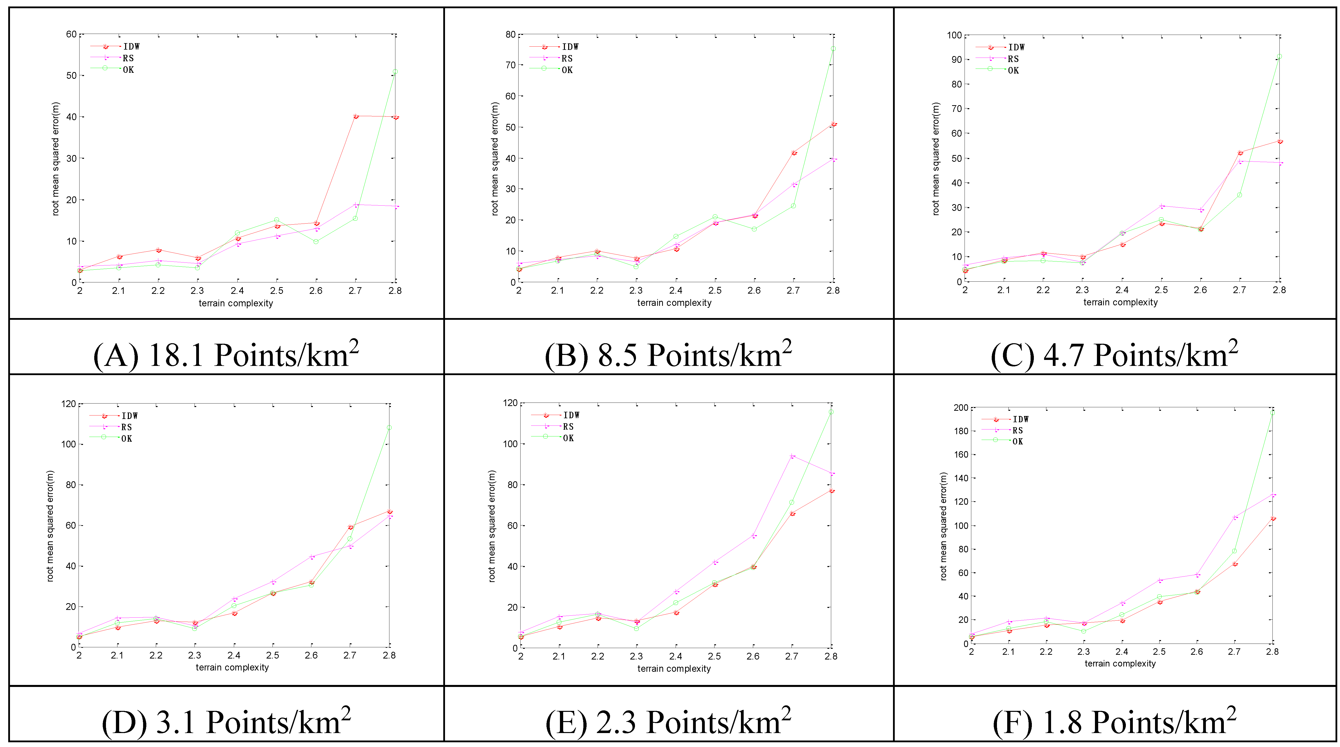
4.4.3. Combined Sampling

For combined sampling, the RMSEs of the three methods shown in Figure 8 and Table 9 have the following patterns:

With the increase of terrain complexity, the RMSEs increase more and more steeply. With the increase of sampling density, the RMSEs decrease, and vice versa. At lower levels of terrain complexity, the OK method has the minimum RMSEs among the three methods, and at higher levels of terrain complexity, the RS method has the minimum RMSEs among the three methods.

4.4.4. Comprehensive Analysis

The statistical analysis of the RMSEs for all sampling modes, nine sampling densities, and six levels of terrain complexity shows the following (Table 7, Table 8 and Table 9).

The RS method has the minimum error among the three methods in the following three cases: (i) regular-grid sampling for all sampling densities and all levels of terrain complexity, (ii) combined sampling for a high level of terrain complexity and all sampling densities, and (iii) selective sampling for a high sampling density and a high level of terrain complexity. The IDW method has the minimum error in selective sampling with low sampling density and low level of terrain complexity, and the OK method has the minimum error among the three methods in the following two cases: (i) combined sampling with all sampling densities and at a low level of terrain complexity, and (ii) selective sampling with a high sampling density and at a low level of terrain complexity.

4.5. Error Variation Trend Analysis

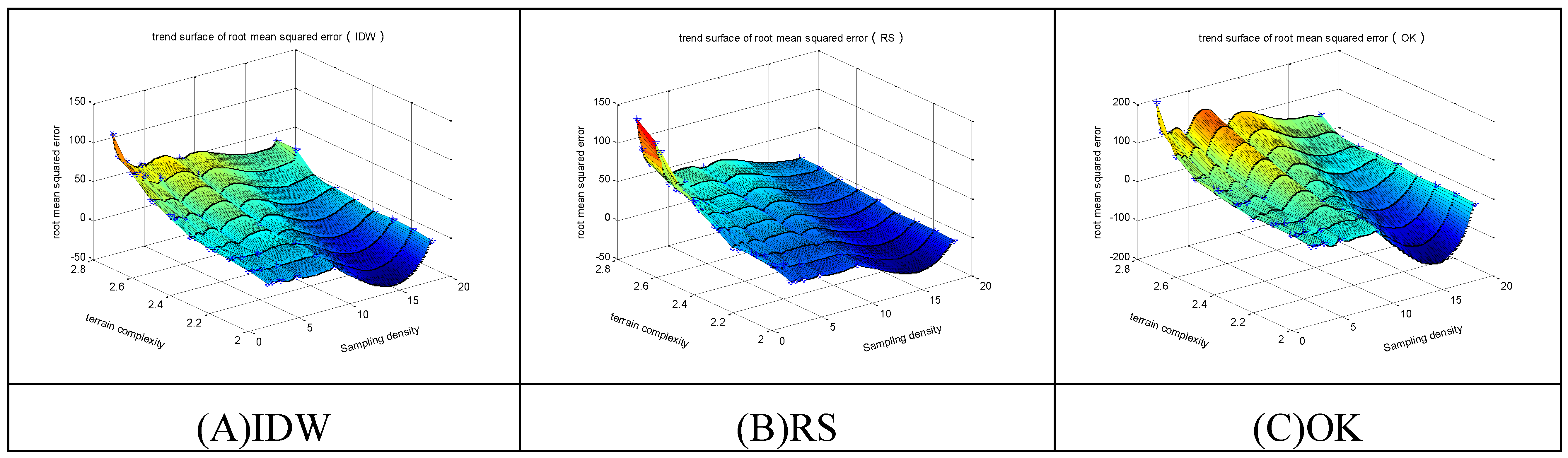
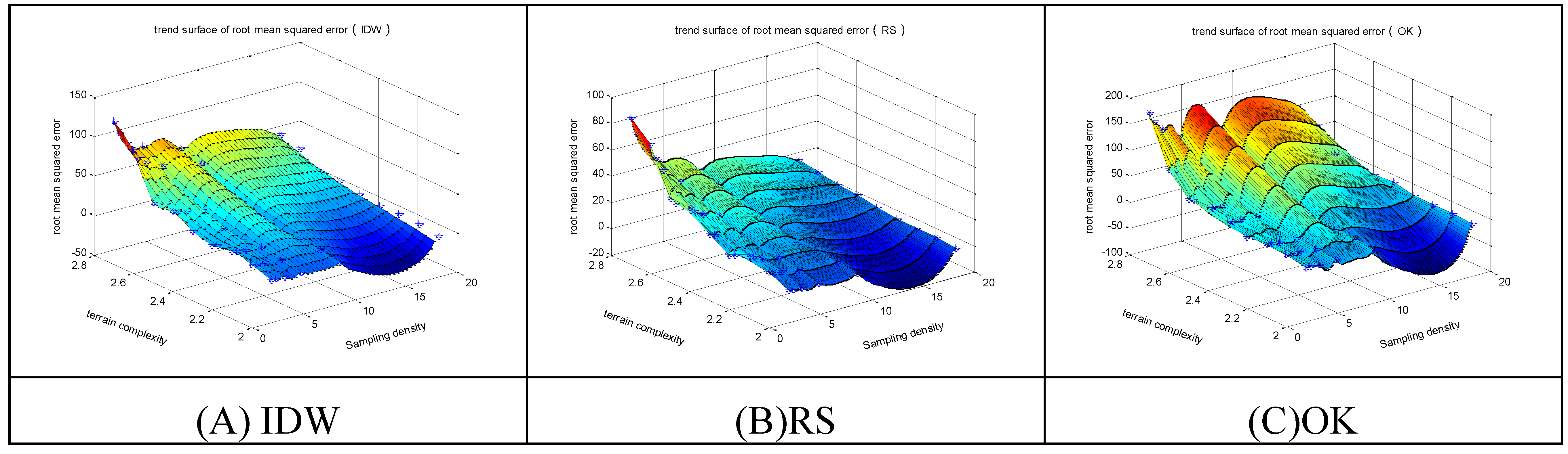
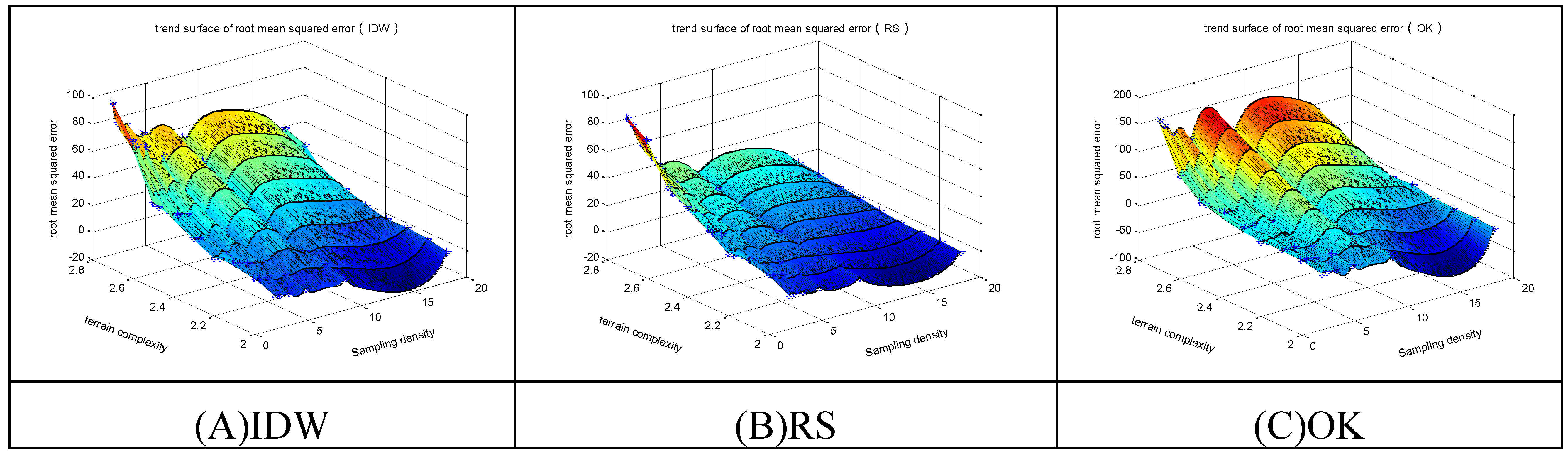
The analysis results of all error indices suggest that the RMSEs satisfy the least squares theory, so this error index is used to represent the accuracy of the interpolation results when analyzing the trend of error variation. Figure 9, Figure 10 and Figure 11 show the following trends of error variation for the three methods.

(1) With the increase of terrain complexity and decrease of sampling density, the accuracy gradually decreases;

(2) For regular-grid sampling, the IDW method has the lowest accuracy, and the OK method has the highest accuracy, approximating the accuracy of the RS method;

(3) For selective sampling, the complicated spatial characteristics of sampling points lead to unstable sampling quality and oscillations of the accuracies of all methods; and

(4) The accuracy of combined sampling is between the other two sampling modes. The IDW method has the lowest accuracy in combined sampling but is better than its accuracy in regular-grid sampling.

Figure 8. The RMSEs of the 3 methods in combined sampling. Sampling densities of (A) 18.1 points/km²; (B) 8.5 points/km²; (C) 4.7 points/km²; (D) 3.1 points/km²; (E) 2.3 points/km²; (F) 1.8 points/km².

Figure 8. The RMSEs of the 3 methods in combined sampling. Sampling densities of (A) 18.1 points/km²; (B) 8.5 points/km²; (C) 4.7 points/km²; (D) 3.1 points/km²; (E) 2.3 points/km²; (F) 1.8 points/km².

Table 9. The RMSEs under combined sampling mode (Unit: m).

	Inverse Distance Weighted Method									Regular Spline Method									Ordinary Kriging Method
	D	2.0	2.1	2.2	2.3	2.4	2.5	2.6	2.7	2.8	2.0	2.1	2.2	2.3	2.4	2.5	2.6	2.7	2.8	2.0	2.1	2.2	2.3	2.4	2.5	2.6	2.7	2.8
SD
18.1		3.0	5.7	7.4	6.7	9.9	15.3	14.9	34.2	39.5	2.9	3.8	4.1	4.2	6.3	8.6	9.9	12.9	14.3	2.6	3.8	4.3	4.1	13.1	10.1	10.0	14.3	52.9
8.5		3.7	7.6	10.1	8.1	12.9	21.0	18.2	43.1	53.3	4.1	6.3	7.2	6.6	10.9	15.5	16.5	22.7	27.3	3.5	5.7	7.0	5.9	15.9	15.4	14.7	30.7	77.1
4.7		4.1	8.5	11.4	9.4	14.9	24.5	22.4	55.2	64.9	5.0	8.7	10.4	8.8	15.9	21.9	23.5	35.6	41.9	4.1	7.5	9.1	7.5	17.9	22.0	19.7	39.3	101.3
3.1		4.5	10.3	12.7	11.4	17.4	28.3	24.8	64.9	74.3	5.6	10.9	13.5	11.8	20.6	28.9	32.0	49.4	59.7	4.5	9.1	11.3	8.9	19.8	26.8	25.2	54.2	120.0
2.3		4.8	10.6	15.3	11.4	18.9	30.2	27.9	67.7	76.6	5.9	12.2	17.6	13.1	22.9	32.3	38.3	58.3	75.5	4.9	10.8	14.4	9.8	21.7	29.2	27.3	64.3	138.7
1.8		4.8	11.5	16.2	12.2	20.0	31.1	32.5	72.1	93.1	5.7	14.2	19.0	16.2	26.8	36.3	44.4	71.8	81.5	4.8	12.4	15.5	10.9	23.0	30.3	33.0	64.8	150.9

Table 9. The RMSEs under combined sampling mode (Unit: m).

	Inverse Distance Weighted Method									Regular Spline Method									Ordinary Kriging Method
	D	2.0	2.1	2.2	2.3	2.4	2.5	2.6	2.7	2.8	2.0	2.1	2.2	2.3	2.4	2.5	2.6	2.7	2.8	2.0	2.1	2.2	2.3	2.4	2.5	2.6	2.7	2.8
SD
18.1		3.0	5.7	7.4	6.7	9.9	15.3	14.9	34.2	39.5	2.9	3.8	4.1	4.2	6.3	8.6	9.9	12.9	14.3	2.6	3.8	4.3	4.1	13.1	10.1	10.0	14.3	52.9
8.5		3.7	7.6	10.1	8.1	12.9	21.0	18.2	43.1	53.3	4.1	6.3	7.2	6.6	10.9	15.5	16.5	22.7	27.3	3.5	5.7	7.0	5.9	15.9	15.4	14.7	30.7	77.1
4.7		4.1	8.5	11.4	9.4	14.9	24.5	22.4	55.2	64.9	5.0	8.7	10.4	8.8	15.9	21.9	23.5	35.6	41.9	4.1	7.5	9.1	7.5	17.9	22.0	19.7	39.3	101.3
3.1		4.5	10.3	12.7	11.4	17.4	28.3	24.8	64.9	74.3	5.6	10.9	13.5	11.8	20.6	28.9	32.0	49.4	59.7	4.5	9.1	11.3	8.9	19.8	26.8	25.2	54.2	120.0
2.3		4.8	10.6	15.3	11.4	18.9	30.2	27.9	67.7	76.6	5.9	12.2	17.6	13.1	22.9	32.3	38.3	58.3	75.5	4.9	10.8	14.4	9.8	21.7	29.2	27.3	64.3	138.7
1.8		4.8	11.5	16.2	12.2	20.0	31.1	32.5	72.1	93.1	5.7	14.2	19.0	16.2	26.8	36.3	44.4	71.8	81.5	4.8	12.4	15.5	10.9	23.0	30.3	33.0	64.8	150.9

Figure 9. The RMSEs of the 3 methods in regular-grid sampling. (A) The trend surface of RMSEs for IDW; (B) The trend surface of RMSEs for RS; (C) The trend surface of RMSEs for OK.

Figure 9. The RMSEs of the 3 methods in regular-grid sampling. (A) The trend surface of RMSEs for IDW; (B) The trend surface of RMSEs for RS; (C) The trend surface of RMSEs for OK.

Figure 10. The RMSEs of the 3 methods in selective sampling. (A) The trend surface of RMSEs for IDW; (B) The trend surface of RMSEs for RS; (C) The trend surface of RMSEs for OK.

Figure 10. The RMSEs of the 3 methods in selective sampling. (A) The trend surface of RMSEs for IDW; (B) The trend surface of RMSEs for RS; (C) The trend surface of RMSEs for OK.

Figure 11. The RMSEs of the 3 methods in combined sampling. (A) The trend surface of RMSEs for IDW; (B) The trend surface of RMSEs for RS; (C) The trend surface of RMSEs for OK.

Figure 11. The RMSEs of the 3 methods in combined sampling. (A) The trend surface of RMSEs for IDW; (B) The trend surface of RMSEs for RS; (C) The trend surface of RMSEs for OK.

5. Discussion

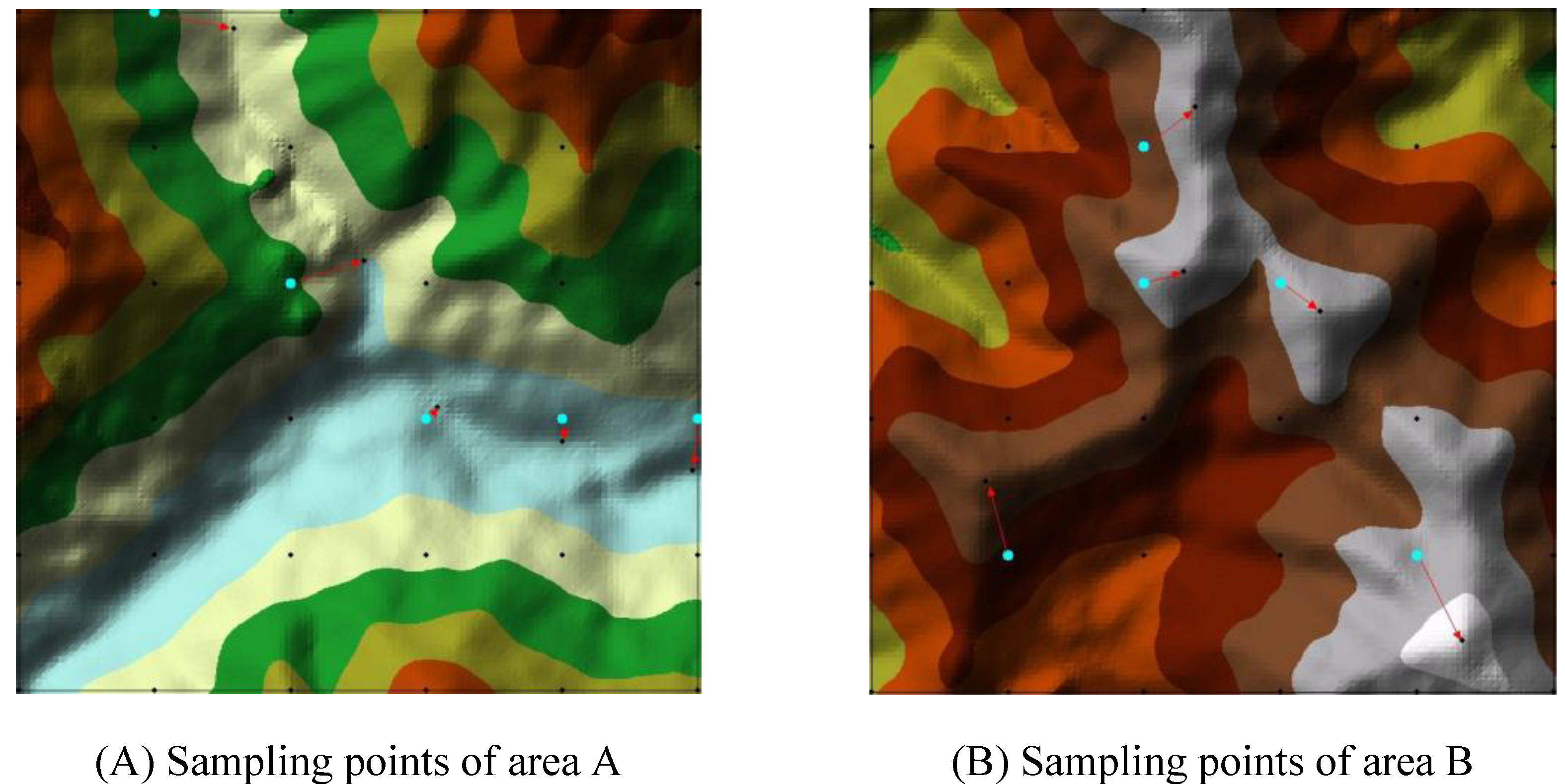
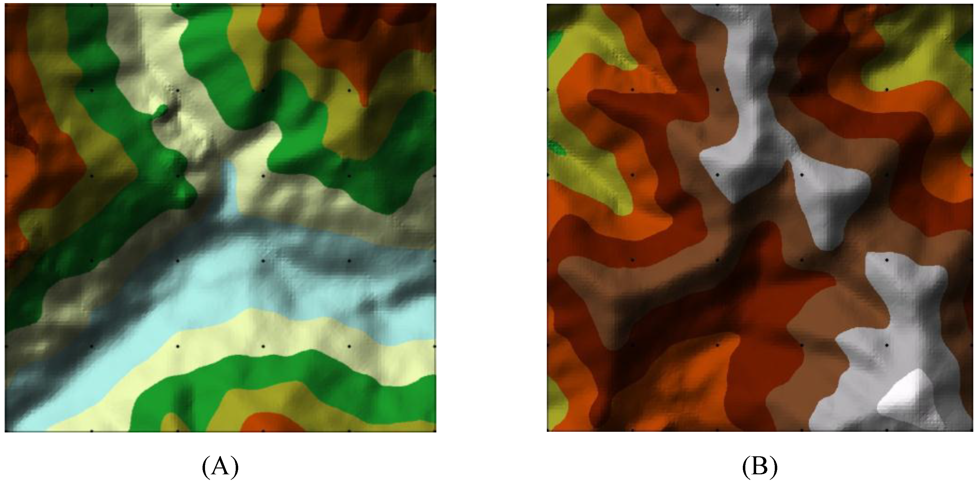
To explain the reasons for the above phenomena, two small regions, A and B in Figure 12, are further examined, using a few sampling points in the regular-grid sampling mode. In combined sampling, the locations of these regular-grid sampling points are modified according to the principles and requirements of the combined sampling mode. In study region A, the sampling points in the mountain valley zone are changed; in study region B, the sampling points in the mountain ridge zone are changed. The details of the modification are shown in Figure 13.

Figure 12. The locations of the sampling points before modification. (A) Sampling points before modification of area A; (B) Sampling points before modification of area B.

Figure 12. The locations of the sampling points before modification. (A) Sampling points before modification of area A; (B) Sampling points before modification of area B.

Figure 13. The locations of the sampling points after modification. (A) Sampling points before modification of area A; (B) Sampling points before modification of area B.

Figure 13. The locations of the sampling points after modification. (A) Sampling points before modification of area A; (B) Sampling points before modification of area B.

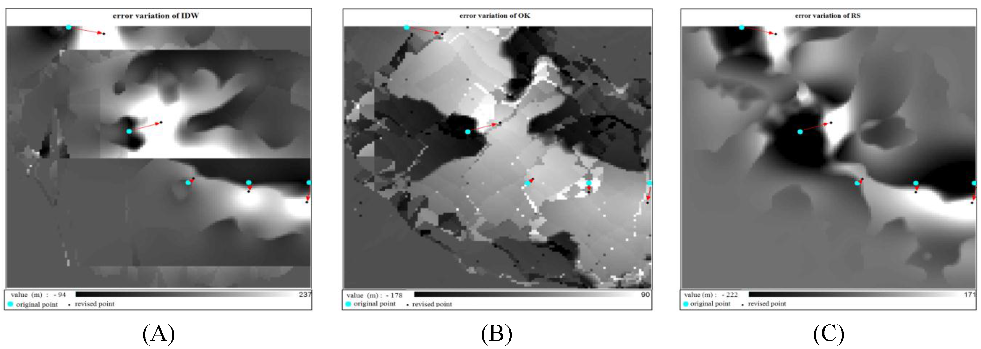
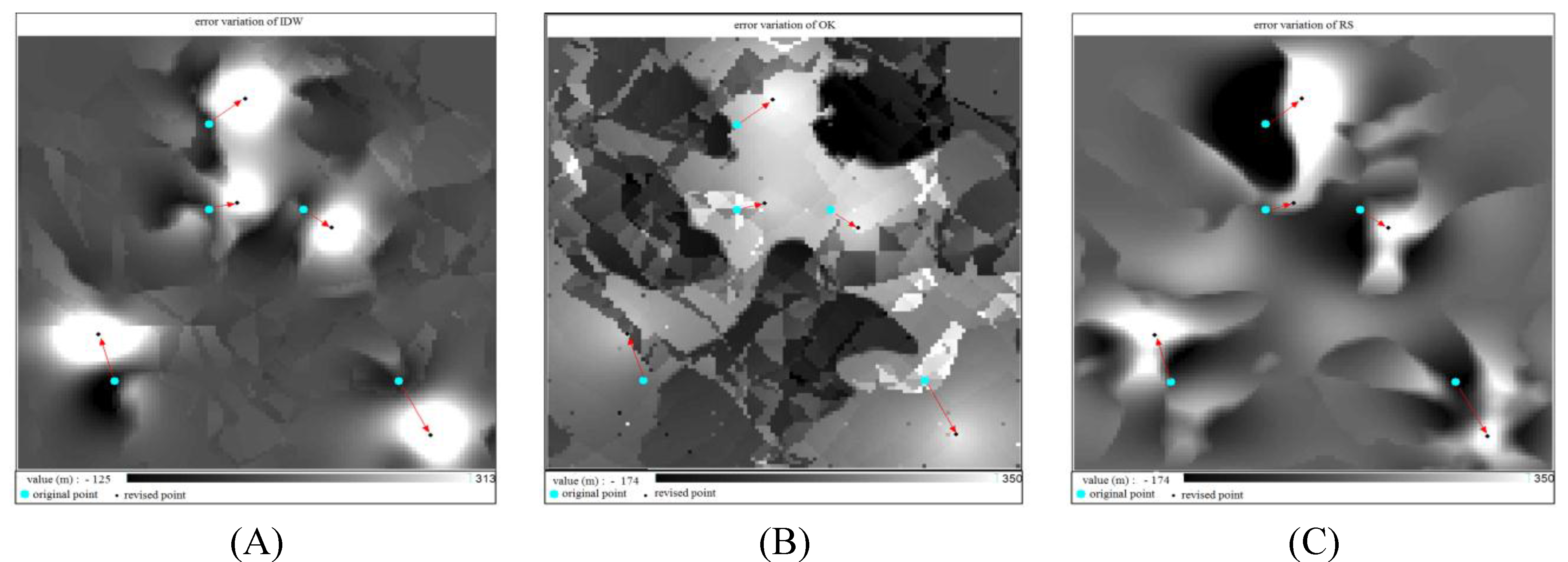
For the two sampling modes, interpolation is conducted on two different sets of sampling points, and the variation of errors at the sampling points (the absolute error before modification subtracted by the absolute error after modification) is shown in Figure 14 and Figure 15. The variation of the errors for the three methods has the following characteristics:

After modification, the errors near the original sampling points are reduced, but the errors near the modified position sampling points are increased. For the IDW method, the area with reduced errors is larger than the area with increased errors, and the reduction is greater than the increase. For the RS method, the area with reduced errors is smaller than the area with increased errors, and the reduction is smaller than the increase.

Figure 14. The variations of the errors at the sampling points of area A. (A) Error variations at the sampling points of IDW in area A; (B) Error variations at the sampling points of OK in area A; (C) Error variations at the sampling points of RS in area A.

Figure 14. The variations of the errors at the sampling points of area A. (A) Error variations at the sampling points of IDW in area A; (B) Error variations at the sampling points of OK in area A; (C) Error variations at the sampling points of RS in area A.

Figure 15. The variations of the errors at the sampling points of area A. (A) Error variations at the sampling points of IDW in area A; (B) Error variations at the sampling points of OK in area A; (C) Error variations at the sampling points of RS in area A.

Figure 15. The variations of the errors at the sampling points of area A. (A) Error variations at the sampling points of IDW in area A; (B) Error variations at the sampling points of OK in area A; (C) Error variations at the sampling points of RS in area A.

The results suggest that when the uniform distribution of sampling points is changed to non-uniform, the accuracy of the IDW method is improved, but the accuracy of the RS method is decreased and the accuracy of the OK method has no significant change.

This phenomenon is analyzed for each method as follows:

For IDW, after point A in Figure 13A is moved to the mountain valley and is assumed to become point B, the accuracy of interpolation is increased by 20 m. The distances between point B and other points are either decreased or increased, assuming that the set of points with increased distance to B is Ω, and the set of points with decreased distance is Φ, occupying area S_Ω and S_Φ, respectively. For large amounts of data points, the number of points and the area of distribution of Ω and Φ are similar, i.e., S_Ω ≈ S_Φ. In area S_Ω, the accuracy of point A is improved, and the weight of each point also increases. Therefore, the accuracy of the entire area is improved. In parts of S_Φ, although the weight of each point decreases, the accuracy at the point A is improved. Moreover, the region from point A to B is flat without mountain valleys or ridges, so the local accuracy is improved or, at most, slightly reduced. Therefore, the overall accuracy is improved.

For RS, uniformly distributed sampling points are fitted with splines with balanced curvatures. When the sampling points are non-uniformly distributed, the curvature of the spline is greater at each sampling point. The interpolation surface may be extended too low or too high, resulting in a rapid increase of errors and a decrease of accuracy.

For OK, multiple factors, including distance and spatial variation, should be considered. Spatial variation is reflected in the variation function, which is selected according to the spatial characteristics of the data points obtained by statistical methods. In this paper, the variation function model is preset. When the sampling mode is changed from regular-grid to selective or combined sampling, the spatial characteristics of the data points are changed accordingly. If the characteristics differ from the preset method, the accuracy of interpolation may not be effectively improved.

6. Conclusions

In this paper, point sets with different spatial characteristics are constructed, and the accuracies of the interpolation results of three commonly used spatial interpolation methods are studied. This study provides guidelines for the selection of interpolation methods and the setting of corresponding parameters.

The experimental results show that the major locations of the interpolation error distribution occur at mountain ridges, valleys, and peaks; the OK method has the largest area of error distribution, which breaks into multiple sections with high sampling density.

The interpolation results of the 3 methods are analyzed with multiple indices (Table 10 and Table 11):

Table 10. The results of the three interpolation methods.

Method	MAX			BIAS			RMSE
	Regular	Selective	Combined	Regular	Selective	Combined	Regular	Selective	Combined
IDW	L	L	M	L	L	L	M	S	M
RS	S	S	S	S	S	S	S	M	S
OK	M	M	L	M	M	M	L	L	L

L means the largest value in the corresponding index; M is the middle value; and S is the smallest value.

Table 10. The results of the three interpolation methods.

Method	MAX			BIAS			RMSE
	Regular	Selective	Combined	Regular	Selective	Combined	Regular	Selective	Combined
IDW	L	L	M	L	L	L	M	S	M
RS	S	S	S	S	S	S	S	M	S
OK	M	M	L	M	M	M	L	L	L

L means the largest value in the corresponding index; M is the middle value; and S is the smallest value.

Table 11. The variation tendency of the interpolation accuracy.

Method	SD↗	TC↘	R–>S	R–>C	S–>C
IDW	↗	↗	↗	↗	↗
RS	↗	↗	↘	↘	↗
OK	↗	↗	→	↘	↗

TC means Terrain Complexity; SD means Sampling Density; ↗ means increase; ↘ means decrease; R–>S means a switch from regular-gird sampling to selective sampling, and R–>C and S–>C have similar meanings.

Table 11. The variation tendency of the interpolation accuracy.

Method	SD↗	TC↘	R–>S	R–>C	S–>C
IDW	↗	↗	↗	↗	↗
RS	↗	↗	↘	↘	↗
OK	↗	↗	→	↘	↗

TC means Terrain Complexity; SD means Sampling Density; ↗ means increase; ↘ means decrease; R–>S means a switch from regular-gird sampling to selective sampling, and R–>C and S–>C have similar meanings.

(1) In the three sampling modes, the RS method has good control of the MAXes, and the other two methods have poor performance;

(2) The RS method has the smallest BIASes, and the IDW method has the largest BIASes for all sampling modes, sampling densities, and levels of terrain complexity. Moreover, all the BIASes are positive values, which illustrates that the three methods have the same problem of over-estimation; appropriate correction should be made for this problem in practical applications, e.g., using a negative-value-offset in the interpolation;

(3) With the increase in sampling density and decrease in terrain complexity, the interpolation accuracy of three methods improves significantly; and

(4) With the change of sampling mode from regular-grid sampling to selective sampling, the IDW method has a significant improvement in interpolation accuracy, but the accuracy of the RS method decreases. With the change of the sampling mode from regular-grid sampling to combined sampling, the IDW method and RS method have the same performance. With the switch of the sampling mode from selective sampling to combined sampling, both the IDW method and the RS method have significant improvements in interpolation accuracy. The interpolation accuracy of the OK method does not change significantly when the sampling mode changes. The performance of the three methods illustrates that selective sampling points have better applicability for IDW than RS. However, a combination between selective sampling and regular-gird sampling is appropriate in practice and can significantly improve the interpolation accuracy. There is no significant dependence of OK method on the sampling mode; a deep spatial analysis for the sampling points should be performed for the use of the OK method.