Geographic Layers as Landscape Drivers for the Marco Polo Argali Habitat in the Southeastern Pamir Mountains of Tajikistan

Abstract

We described in this report the essential geographic layers used as landscape drivers for the Marco Polo Argali habitat in the eastern Tajik Pamirs. Using remote sensing techniques and geographic information systems (GIS), individual layers were generated in order to acquire more information on argali patterns and habitat suitability and to make the dataset available online. We introduced an improved object-based image analysis in our mapping of the vegetation cover by utilizing spectral, topographic, and texture variables. We exhausted every Landsat image band and texture feature combination to select the best pairing of band-texture components. For vegetation class alone, the producer’s accuracy was 90.8% and the user’s accuracy was 91.6%.

1. Introduction

The Marco Polo argali (Ovis ammon polii) is a subspecies of argali (Ovis ammon), and is considered the longest-horned species of wild sheep. Named after the explorer Marco Polo and first described scientifically in 1841 by Edward Blyth, Marco Polo argali occurs in the Tajikistan Pamir Mountains [1], as well as in limited regions in China, Afghanistan, Pakistan, and Kyrgyzstan [2]. Due to the sheep’s impressive horn, foreign hunters are willing to pay large amounts of money for a hunt [3]. In fact, in a report by Luschekina [4] covering the years 1967 to 1989, a total of $20 million was paid by wealthy trophy hunters. Recent studies on the status of the argali population have shown a decline in numbers [5,6] caused by trophy hunting and subsistence poaching [7]. O. ammon has been categorized in several lists, such as the Appendix II of CITES and the 2000 IUCN Red List, as vulnerable or threatened species. O. Aknazarov, Pamir Biological Institute Director, said that the total number of Marco Polo sheep in the Tajik Pamirs may only be between 3000 to 5000 animals. Valdez et al. [2], however, counted a total of 8649, 8392, and 7663 sheep in a four-year successive surveys from 2009 to 2012. Argalis usually inhabit the rolling hills that lack tall vegetation to visually scan for predators [8]. They also prefer rugged mountainous landscapes for escape cover and relies on speed for evading predators [9].

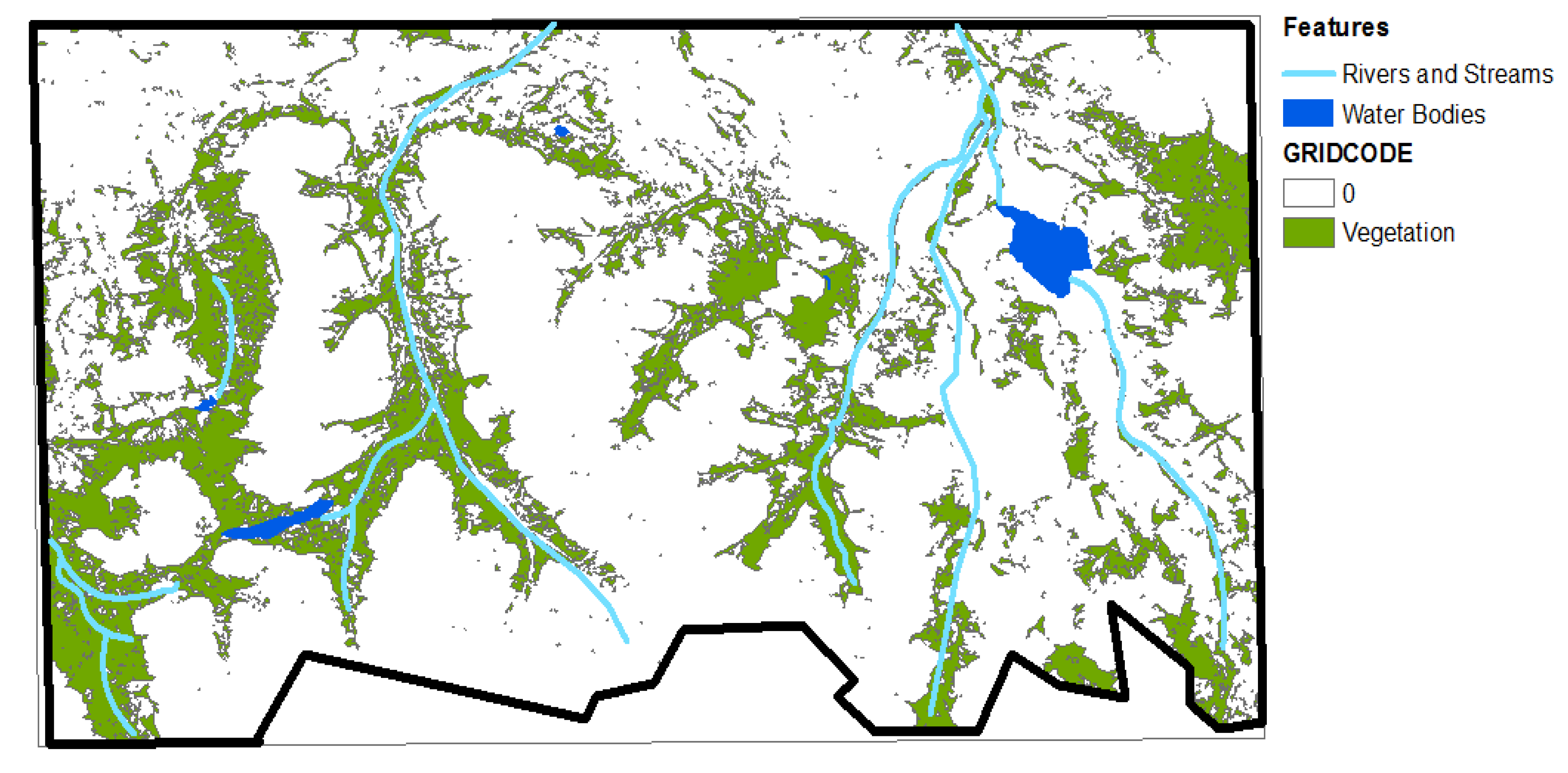
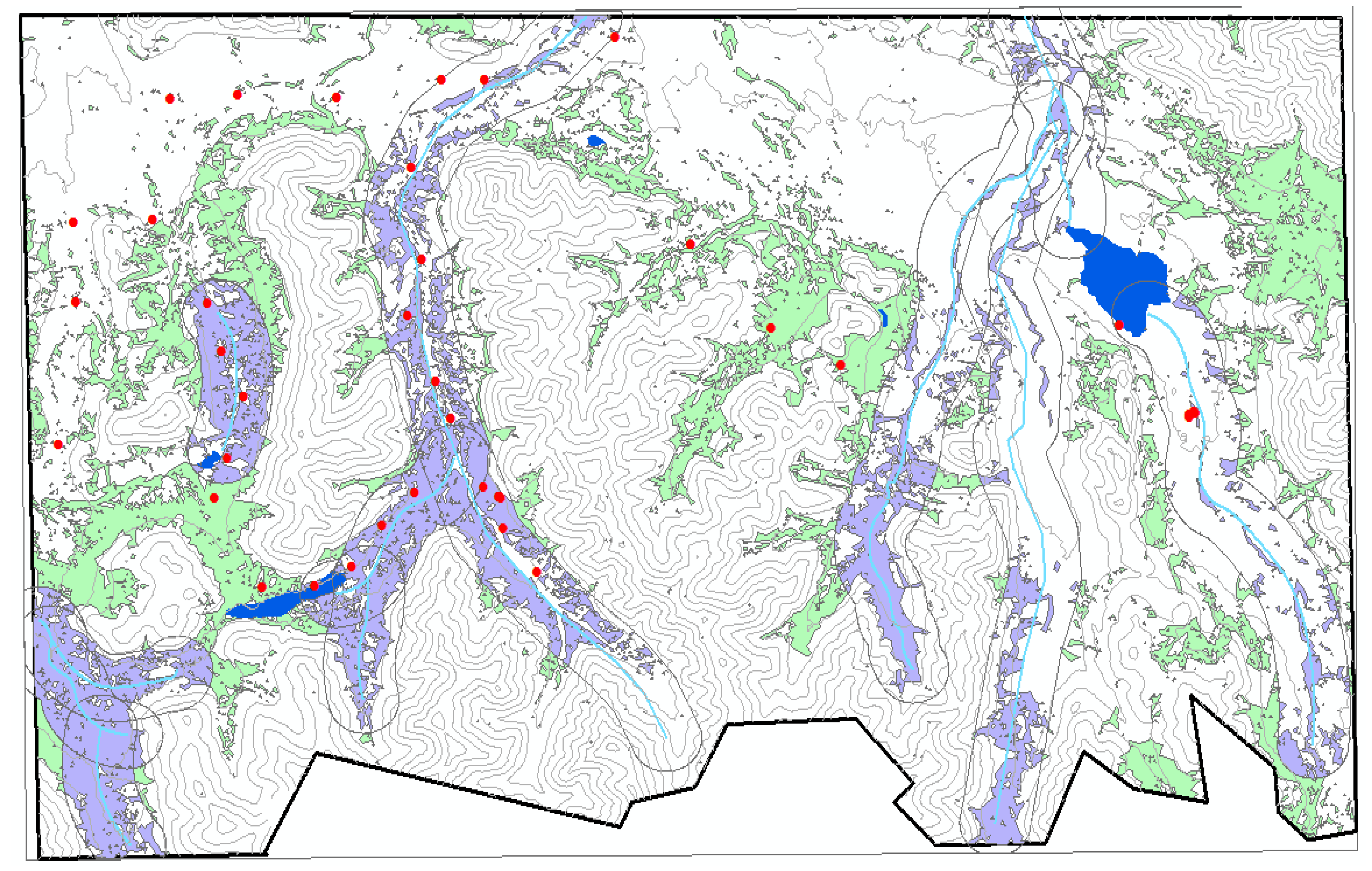
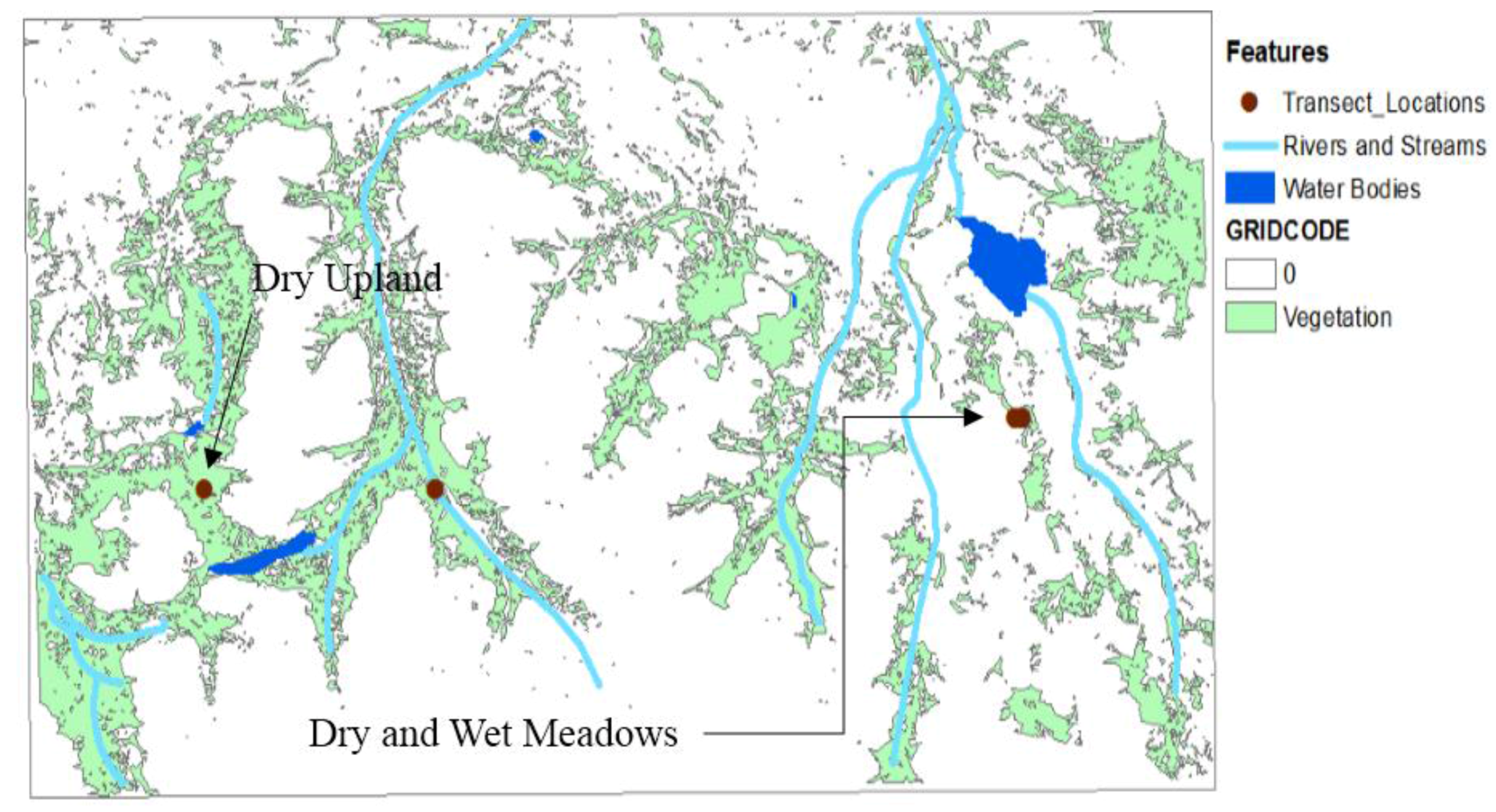
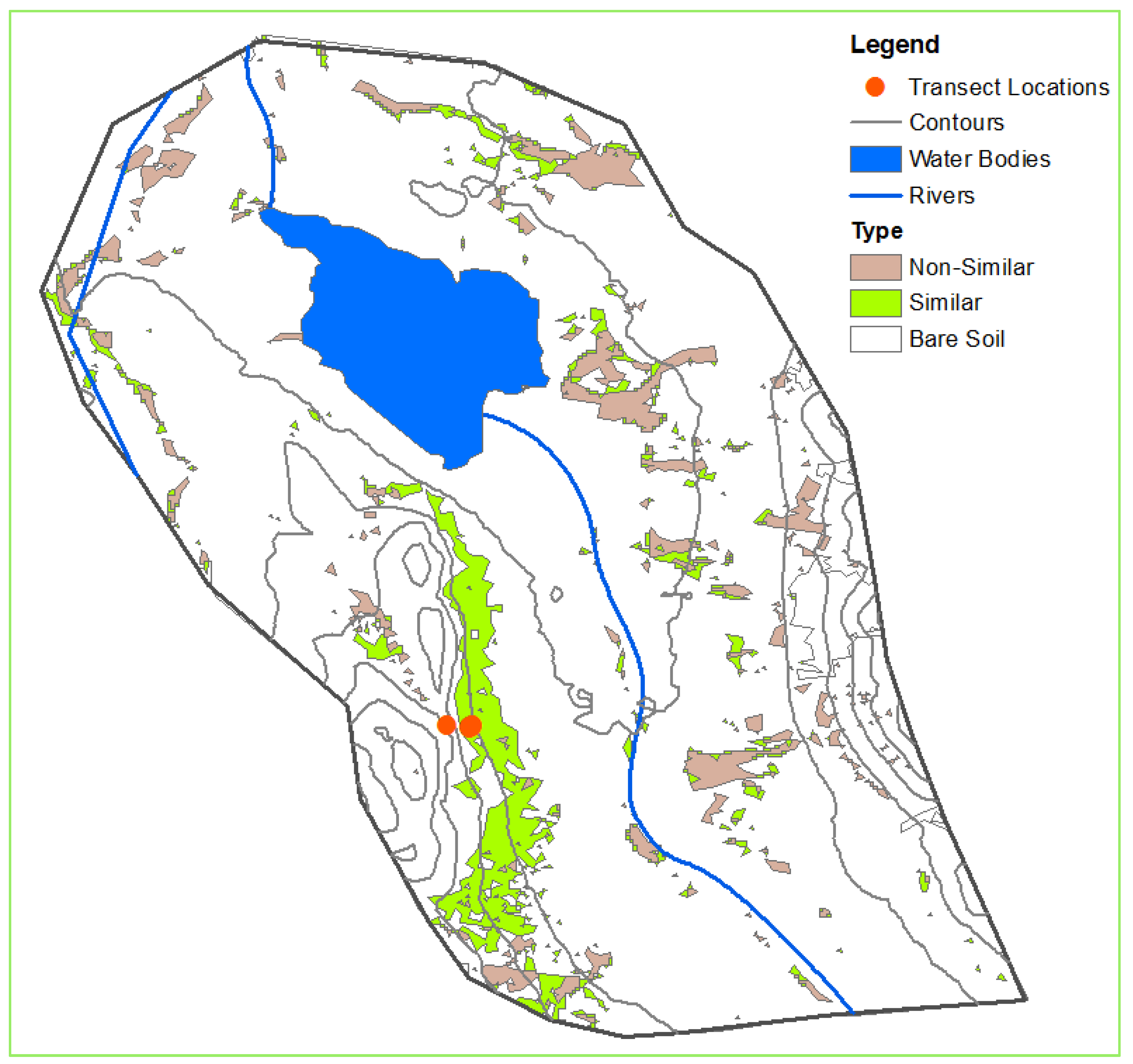
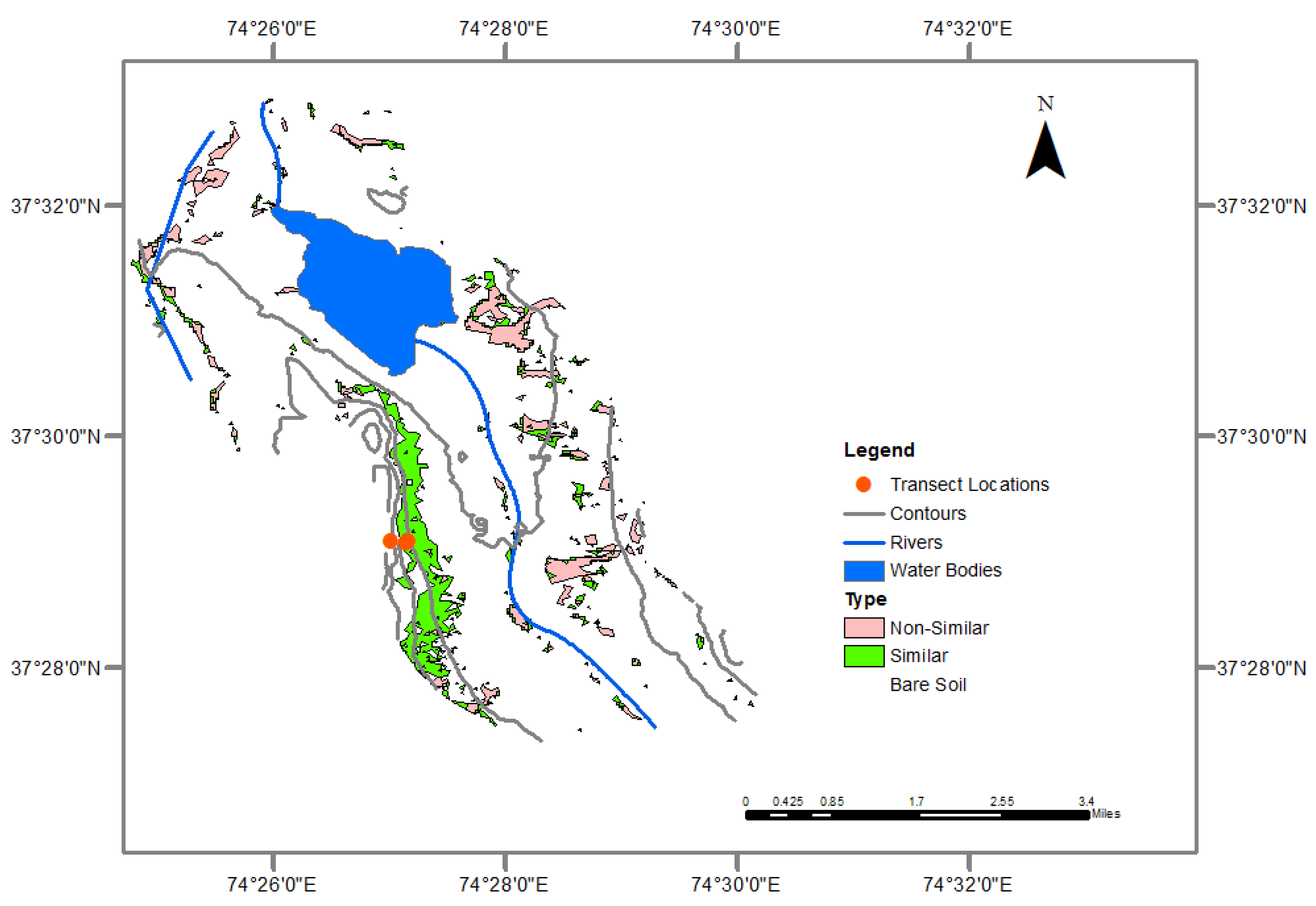
In this report, we described a small portion of our study area in the southeastern Tajik Pamirs that contained the two available datasets—one dataset listed the occupancy locations of wild sheep, and the second dataset detailed transect surveys that showed surface characteristics of possible sheep habitat. Using remote sensing techniques and geographic information systems (GIS), descriptions of the sheep habitat were presented in GIS layers. We generated individual layers to obtain information on argali patterns and habitat suitability and to make the dataset available online to the rest of the research community.

2. Study Area

The area of interest (Figure 1) is located in the southeastern Pamir Mountains of Tajikistan in the Gorno-Badakhshan Autonomous Region, between the latitudes 37°N to 38°N and longitudes 74°E to 75°E and covers an area of approximately 2223 km² (223,000 ha). The rocky mountainous terrain has an altitude of 3500 m to 5500 m (11,480 to 18,000 ft) above mean sea level (amsl). The study area roughly corresponds to the area of a wild ungulate hunting concession in which 45 hunting permits are issued yearly at a cost of $40,000 per permit. Aside from the argali, another wild ungulate, the Asiatic ibex (Capra sibirica), exists in the area [2].

Figure 1. The smaller study area of interest is located in the southeastern region of Tajikistan and based on a single Landsat scene.

Figure 1. The smaller study area of interest is located in the southeastern region of Tajikistan and based on a single Landsat scene.

Average annual precipitation is about 100 mm (3.9 in) with sub-zero average temperatures from October to March. With such extreme climate conditions, herding of yaks, sheep, and goats has been the primary agricultural option [10] with domestics being the most numerous. Domestic animals are transported to lower pastures during the fall, winter, and early spring (October–May) to avoid the harsh winter weather. The summer pastures are dominated by Artemisia and Festuca species, with productivity of 0.3 to 0.4 t∙ha^–1 and 0.8 to 1.2 t∙ha^–1, respectively [11]. Grazing competition between wild ungulates and livestock can be found on pastureland near human settlements [12,13].

3. Data and Methodology

Systematic description of data processing steps is presented here:

(1) Preprocessing of the Landsat image to enhance the quality of the data and to remove noise caused by internal and external conditions and eliminate other undesirable characteristics produced by the sensor.

The 30-m spatial resolution Landsat 7 Enhanced Thematic Mapper Plus (ETM+) image from July 2012 was used for the analysis to coincide with the date of the fieldwork. The level-1 terrain-corrected product (L1T) Landsat time-series data were obtained from the U.S. Geological Survey Earth Resources Observation and Science (USGS EROS) resource archive (http://eros.usgs.gov/). The month of July is within the period identified to be the vegetation response peak [14]; the time of year when the development stage of the vegetation produces the highest spectral signals. Using ERDAS Imagine [15], we normalized the image by converting the measured digital number (DN) values to top of atmosphere (TOA) reflectance units [16].

(2) Screening of cloud patches, cloud shadows, and snow were performed to ensure that the image was devoid of obstructions that may result in false classification of the vegetation cover.

We did visual and/or spectral examinations of the image to assess for cloud presence and shadow contaminations, delineated them and then masked out from the analysis. Most of the contaminations were found south of the Landsat scene. Since our study area was located near the center of the scene, we managed to avoid 95% of the cloud cover and snow. Thus, clouds, shadows, and snow cover were not major constraints in the image processing. For the snow mask, we created the Normalized Difference Snow Index (NDSI) [17] image to distinguish snow from other surrounding features. A threshold was applied to the NDSI to filter the non-snow features that may have been misclassified as snow by examining reflectance at other wavelengths. Further, we did extensive manual deleting of isolated snow artifacts especially in transition areas between snow and non-snow features located on steep slopes.

(3) The integration of the variables such as digital elevation model (DEM), Normalized Difference Vegetation Index (NDVI), Principal Component Analysis (PCA), Modified Soil-adjusted Vegetation Index (MSAVI), and texture features into the object-based image classification analysis.

Instead of the pixel-based method, we utilized the object-based image analysis (OBIA) for our image classification, guaranteeing a much higher classification accuracy [18,19,20,21]. OBIA is appropriate to capture the landscape patterns and derive the dynamics of neighboring objects.

Spectral and topographic variables, namely, NDVI [22], PCA [23], MSAVI [24], and DEM [25], were integrated with texture features such as homogeneity (HOM), second moment (M2), dissimilarity (DIS), entropy (ENT), and contrast (CON), for the object-based classification. Few studies have noted that the addition of DEM, NDVI, PCA, and MSAVI could help improve image classification results in terms of feature discrimination and accuracy of featured classes (e.g., [26,27]). We utilized the DEM from NASA’s Shuttle Radar Topography Mission (SRTM) 90-m digital elevation online dataset via the USGS website (http://srtm.usgs.gov/index.php). We rescaled the DEM to the spatial resolution of the spectral variables (30 m). Further, we added the individual Landsat bands 4 and 5 NIR data space to ensure clear separation between vegetation surfaces and soil [28].

For the texture variables, we took advantage of ENVI software’s textural filters that were based on the co-occurrence measures [29]. The measures use a matrix to calculate the texture values within the processing window. The matrix gives the instances of occurrences of the relationship between a pixel and its specified neighbor. A number of studies had shown improved land use and land cover (LULC) classification accuracy when using the texture images in OBIA (e.g., [30,31]). Stefanov et al. [32] and Pesaresi et al. [33] used a single band to compute the texture components. In this study, we exhausted every Landsat band and texture feature combination to select the best pairing of band-texture components. A package called FactoMineR was run in the R environment to show opposing vectors, which could designate the best spectral band or bands that will be employed for each particular texture image. Opposing vectors indicate that the components are negatively correlated and considered as best variable candidates for the classification. Once all variables for OBIA were computed, partitioning of the image into segments followed. The result was a segmentation image, where each zone is assigned the computed spectral values of all the pixels that belong to that zone.

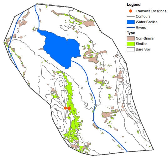
Within ENVI’s Feature Extraction module, we applied the k-nearest neighbor (KNN) method to classify the image. We limit the land use classes to only three: vegetation, water, and barren land as our objective was to specifically delineate the summer vegetation cover only. These three classes were not difficult to identify from the Landsat image. For the training data, we relied on the Google Earth engine, the expert knowledge of the area, the spectral signatures of the classes, and the data collected from the field survey in 2012. In addition, reference points from high resolution images of QuickBird (60-cm resolution) and WorldView-2 (50-cm resolution) were tapped to aid in the identification and assigning of classes. As a note, we only used 75% of the points we collected (550 points in total) for training. The remaining 25% was used for classification validation.

We assessed the accuracy of our image classification using overall accuracy (OA), producer’s accuracy (PA), user’s accuracy (UA), and kappa coefficient. We looked at the agreement between the classified image and the reference map; a kappa statistics value of 0.4 means poor agreement, while excellent agreement should have a value of more than 0.85. Any value in between is considered fair to good.

(4) Derivation of secondary raster datasets such as slope, aspect, and river networks.

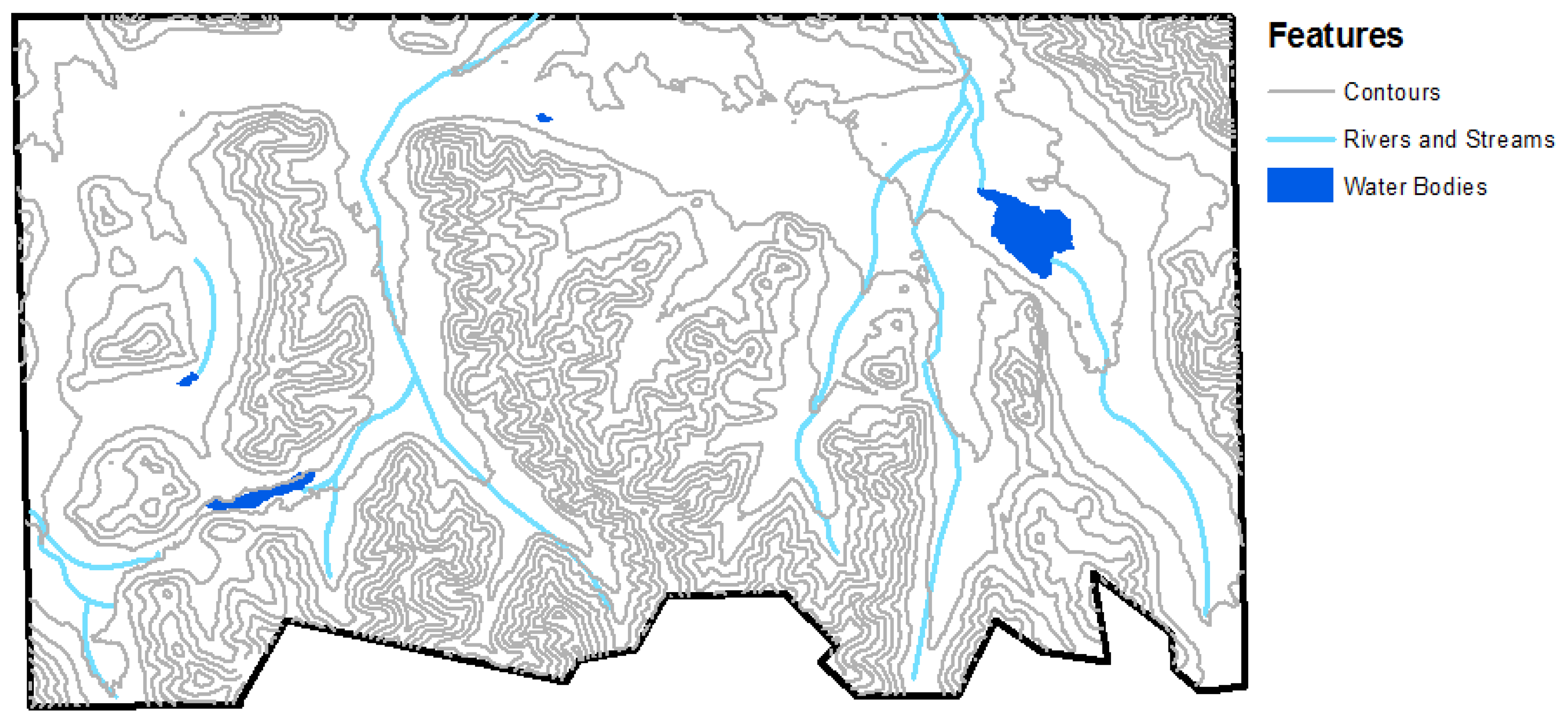
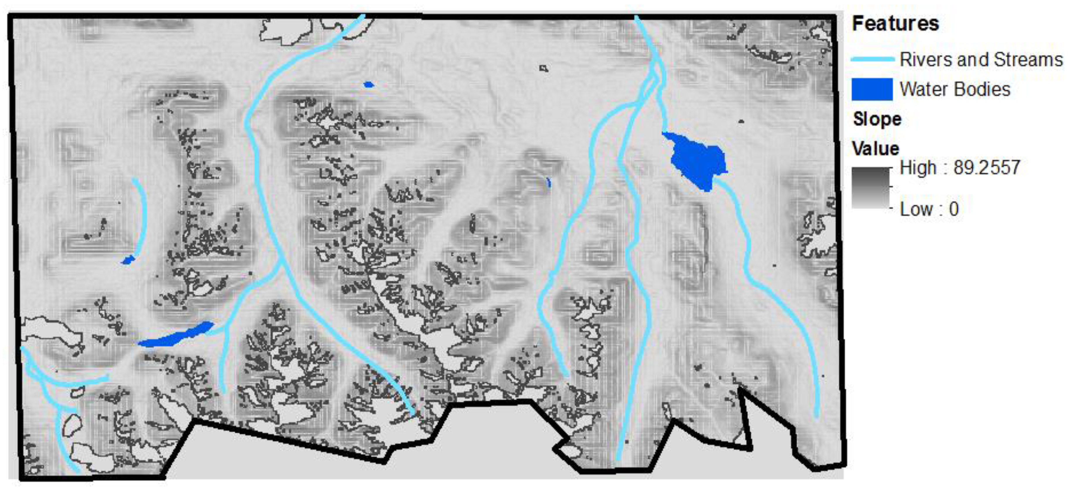
From the DEM dataset, we derived the slope, aspect, and the TIN, using ArcGIS software.

(5) Overlaying of various vector layers, deriving descriptive statistics using GIS-based analysis, and showing necessary maps.

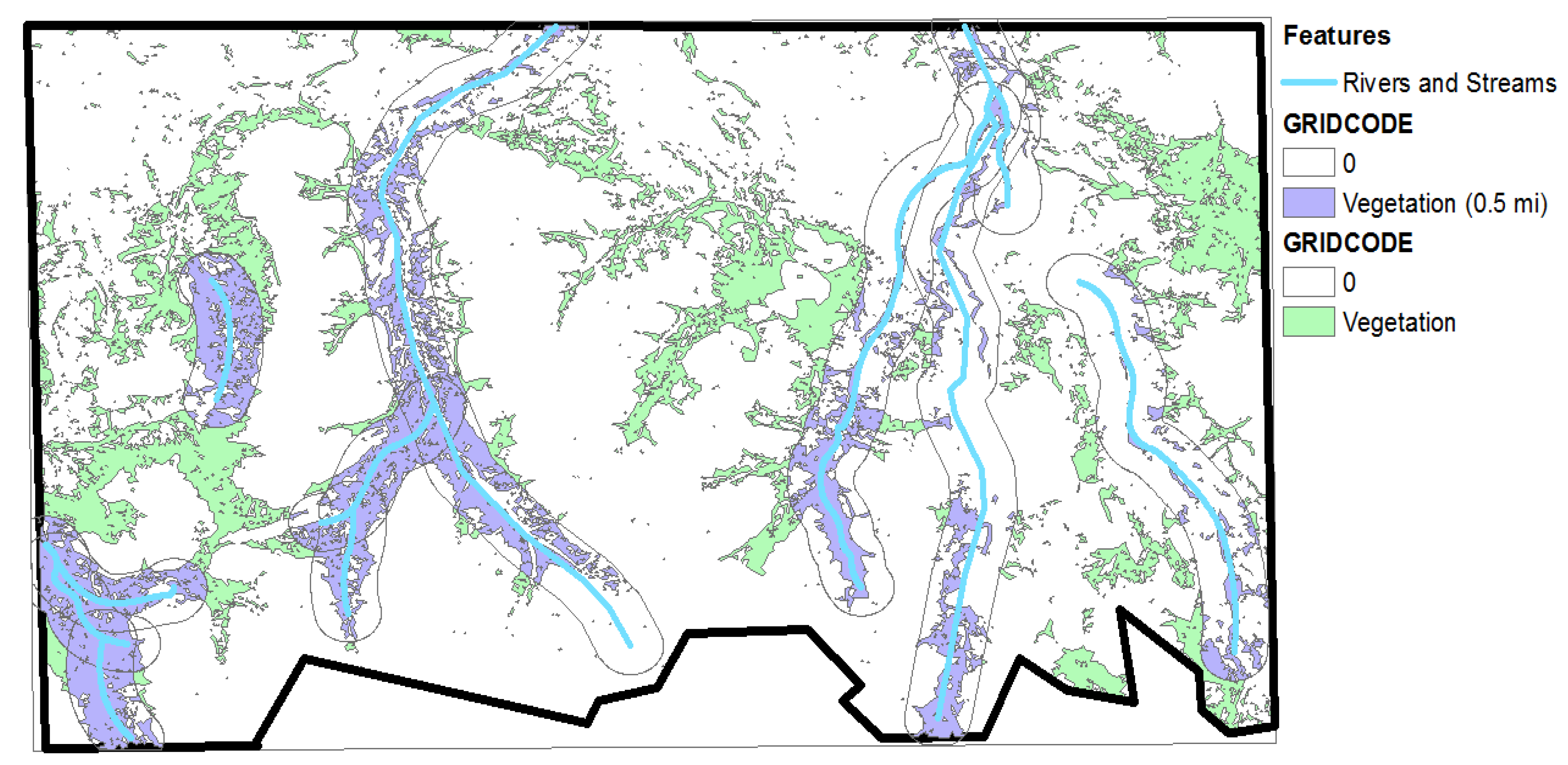
The list of layers we derived and analyzed were rivers and streams, water bodies, topography, and vegetation cover. In this report, rivers and streams refer to riparian areas, which may not have flowing water throughout the year. A layer for human settlements was not included as nothing was detected in the study area. We tabulated the results of our analysis.

4. Results and Discussion

We divided this report into sections according to each principal geographic information layer or driver. A driver is an entity that can be mapped or spatially delineated on the landscape, which we then manipulated and analyzed.

4.1. Rivers and Streams Network

The total length of rivers and streams combined was about 92.32 km (57.37 mi) (Figure 2). Of this length, 38.83 km (24.13 mi) were from two major rivers.

Figure 2. The study area in the eastern Pamir Mountains with the river and stream network and the major water bodies.

Figure 2. The study area in the eastern Pamir Mountains with the river and stream network and the major water bodies.

4.2. Water Bodies

The major water bodies are shown in Figure 2. The area of the largest lake located in the northeast region of the study area was about 3.24 km² (324 ha). The rest of the inland water sources had areas that range from 0.08 to 1.04 km² (7.8 ha to 104 ha).

4.3. Topography

Descriptive statistics of the topography are summarized in Table 1. The mean elevation seen was 4430 m (14,534 ft) amsl. The maximum degree of slope inclination observed was high at 89.26°, indicating the presence of essentially vertical inclinations in the area. In fact, about 9% of the area was considered very steep, with a slope greater than 80° (Table 2). The minimum degree of slope inclination was 0.27°, indicating flat areas on valleys and foothills. Nearly half of the study area (48.9%) was within 1° to 10° slope. Evidence of slopes gradually increasing was reflected in Table 2: from 11° to 20° (15.3%), to 21° to 30° (15.5%), to 31° to 40° (6.4%). Figure 3 shows the slope map of the study area.

Figure 3. The slope map of the study area in the eastern Pamir Mountains (in degrees). The maximum degree of slope inclination is 89.26°, while the minimum is 0.27°.

Figure 3. The slope map of the study area in the eastern Pamir Mountains (in degrees). The maximum degree of slope inclination is 89.26°, while the minimum is 0.27°.

Table 1. Minimum, maximum, and mean values of landscape properties of the study area in the eastern Pamir Mountains.

	Elevation (m/ft)	Slope (°)	Aspect (°)
Minimum	4133/13,560	0.27	−1 (Water bodies)
Maximum	5232/17,165	89.26	359
Mean	4430/14,534	44.76	137

Table 1. Minimum, maximum, and mean values of landscape properties of the study area in the eastern Pamir Mountains.

	Elevation (m/ft)	Slope (°)	Aspect (°)
Minimum	4133/13,560	0.27	−1 (Water bodies)
Maximum	5232/17,165	89.26	359
Mean	4430/14,534	44.76	137

Table 2. Percent distribution of the slope inclination in the Pamir Mountains study area.

Inclination (°)	<1	1–10	11–20	21–30	31–40	41–50	51–60	81–90	Total
Count	20,345	218,953	68,343	69,492	28,715	1642	371	40,141	448,002
%	4.5	48.9	15.3	15.5	6.40	0.40	0.08	8.92	100

Table 2. Percent distribution of the slope inclination in the Pamir Mountains study area.

Inclination (°)	<1	1–10	11–20	21–30	31–40	41–50	51–60	81–90	Total
Count	20,345	218,953	68,343	69,492	28,715	1642	371	40,141	448,002
%	4.5	48.9	15.3	15.5	6.40	0.40	0.08	8.92	100

4.4. Vegetation Cover

The texture variables b5HOM (homogeneity computed from band 5) and b5CON (contrast computed from band 5) plus the spectral/topographic variables DEM, NDVI, and b4 produced the best segmentation performance. The set was then used in the segmentation process, and eventually, in the final image classification. The classified map showed an overall accuracy of 91.8%, and a kappa statistic of 0.85. For vegetation class alone, the PA was 90.8% and the UA was 91.6%.

The total area covered by vegetation was about 146 km² (14,600 ha) (Figure 4), which was approximately 23% of the total study area. More than 80% of the vegetative cover was located within 2 mi from rivers and streams (Table 3), and within valleys and on foothills. Additionally, about 42% of the vegetation was within a distance of 0.5 mi from the river. A small percentage of vegetation cover (2.3%) thrived 4 mi away from rivers.

Figure 4. Vegetation cover map of the study area in the eastern Pamir Mountains. Vegetation is concentrated more on the valleys and foothills, and near rivers and streams.

Figure 4. Vegetation cover map of the study area in the eastern Pamir Mountains. Vegetation is concentrated more on the valleys and foothills, and near rivers and streams.

Table 3. Percentage of vegetation cover in river buffer zones in the eastern Pamir Mountains.

Distance From River (mi/km)	Area (km2/ha)	Percentage (%)
0.5 (0.80)	62.04 (6203.97)	42.28
1.0 (1.61)	30.34 (3034.44)	20.68
2.0 (3.22)	30.71 (3071.45)	20.93
3.0 (4.83)	20.14 (2013.63)	13.72
4.0 (6.44)	3.38 (337.94)	2.30

Table 3. Percentage of vegetation cover in river buffer zones in the eastern Pamir Mountains.

Distance From River (mi/km)	Area (km2/ha)	Percentage (%)
0.5 (0.80)	62.04 (6203.97)	42.28
1.0 (1.61)	30.34 (3034.44)	20.68
2.0 (3.22)	30.71 (3071.45)	20.93
3.0 (4.83)	20.14 (2013.63)	13.72
4.0 (6.44)	3.38 (337.94)	2.30

What percentage of vegetation cover fell on lower elevation? In Table 4, only 8.48% of vegetation cover fell in the lower elevation of 4200 m (13,780 ft) amsl. About 40% of the vegetation was at 4400 m (14,436 ft) amsl. Overall, 97% of the areas covered with vegetation were at elevations 4600 m (15,092 ft) amsl and below.

Table 4. Percentage of vegetation cover that is situated in various elevations of the study area in the eastern Pamir Mountains.

Elevation (m/ft)	Percentage (%)
4200 (13,780)	8.48
4300 (14,108)	30.27
4400 (14,436)	40.75
4500 (14,764)	14.47
4600 (15,092)	3.47
4700 (15,420)	0.82
4800 (15,748)	0.07
4900 (16,076)	0.03
5000 (16,404)	0.01
5200 (17,060)	0.90

Table 4. Percentage of vegetation cover that is situated in various elevations of the study area in the eastern Pamir Mountains.

Elevation (m/ft)	Percentage (%)
4200 (13,780)	8.48
4300 (14,108)	30.27
4400 (14,436)	40.75
4500 (14,764)	14.47
4600 (15,092)	3.47
4700 (15,420)	0.82
4800 (15,748)	0.07
4900 (16,076)	0.03
5000 (16,404)	0.01
5200 (17,060)	0.90

Figure 5. Vegetation cover map of the study area showing the portion of vegetation (42.28%) falling within the 0.5 mi (0.80 km) river buffer zone.

Figure 5. Vegetation cover map of the study area showing the portion of vegetation (42.28%) falling within the 0.5 mi (0.80 km) river buffer zone.

In Table 3, about 42.28% of the total vegetation cover was within 0.5 mi (0.80 km) from the river. This percentage was further classified in Table 5. Close to 50% (49.81%) of the vegetation within the 0.5 mi buffer zone fell on 4400 amsl.

Table 5 shows that the range of elevations for zones 0.5 mi from the river is from 4200 m to 4700 m (13,780 to 15,420 ft). See map in Figure 5 of all vegetation cover within the 0.5 mi river buffer zone.

Table 5. Percentage of vegetation cover at elevations within 0.5 mi (0.80 km) from the river.

Elevation (m/ft)	Percentage (%)
4200 (13,780)	10.83
4300 (14,108)	29.21
4400 (14,436)	49.81
4500 (14,764)	8.83
4600 (15,092)	1.25
4700 (15,420)	0.08

Table 5. Percentage of vegetation cover at elevations within 0.5 mi (0.80 km) from the river.

Elevation (m/ft)	Percentage (%)
4200 (13,780)	10.83
4300 (14,108)	29.21
4400 (14,436)	49.81
4500 (14,764)	8.83
4600 (15,092)	1.25
4700 (15,420)	0.08

4.5. Marco Polo Argali Occupancy

Locations of Marco Polo sheep occupancy were recorded through fieldwork in the summers of 2010 and 2012. Figure 6 shows locations of the recorded occupancies of Argalis in the study area. Of the 41 locations, 28 (or 68.29%) were within the 0.5 mi (0.80 km) river buffer zone (Table 6). Needless to say, Argalis at these 28 locations have easy access to rivers/streams and the majority of the vegetation cover (42.28% in Figure 6) at lower elevations, 4200 m to 4700 m (13,780 to 15,420 ft) (Table 5).

Figure 6. Occupancy of Marco Polo Argali (red dots) in the study area, eastern Pamir Mountains, Tajikistan.

Figure 6. Occupancy of Marco Polo Argali (red dots) in the study area, eastern Pamir Mountains, Tajikistan.

Table 6. Percentage of the Argali locations relative to river buffer zones.

Distance From River (mi/km)	No. of Argali Locations	Percentage (%)
0.5 (0.80)	28	68.29
1.0 (1.61)	2	4.87
2.0 (3.22)	4	9.75
3.0 (4.83)	5	12.20
4.0 (6.44)	2	4.87

Table 6. Percentage of the Argali locations relative to river buffer zones.

Distance From River (mi/km)	No. of Argali Locations	Percentage (%)
0.5 (0.80)	28	68.29
1.0 (1.61)	2	4.87
2.0 (3.22)	4	9.75
3.0 (4.83)	5	12.20
4.0 (6.44)	2	4.87

4.6. Transect Data Analysis

Plant data were collected via the transect method in the summer of 2012. Transects were located in dry and wet meadow, and in dry upland environments (Figure 7).

The wet meadow plant community consisted of majority 44.2% of grasses/sedge and 43.87% sheep droppings. The most diverse vegetative class in the dry meadow was Forbs with 13.63% cover observed and sheep droppings was recorded as 13.9%. The wet and the dry meadows were about 27.34 m (0.017 mi) apart. Aside from the wet meadow, the dry upland also recorded a high percentage of sheep droppings at 43.87%.

The wet meadow is popular for sheep during the winter season, while the dry upland is used in the spring. The dry upland is characterized by steep terrain, which ewes and lambs use as escape terrain. In our analysis, the wet meadow comprised a flatter slope compared to the dry meadow and the dry upland locations (Table 7). The dry upland was located at about 4380 m (14,370 ft) amsl; 55 m (181 ft) higher than the dry meadow and 76 m (249 ft) higher than the wet meadow. In terms of escape terrains for the sheep, the dry upland was bounded by steeper terrains in the northeast and southwest directions. The location of the dry upland community was less than 160 m to the next 100 m (higher) elevation.

Figure 7. Locations of the transect dataset collected in 2012. The inset shows the wet and dry meadow points.

Figure 7. Locations of the transect dataset collected in 2012. The inset shows the wet and dry meadow points.

Table 7. Location of transects in reference to landscape features in the study area, eastern Pamir Mountains, Tajikistan.

	Wet Meadow	Dry Meadow	Dry Upland
Slope (%)	0.0	13.0	4.70
Elevation (m)	4314	4325	4380
Distance From River (mi)	0.836980	0.84915	1.14236

Table 7. Location of transects in reference to landscape features in the study area, eastern Pamir Mountains, Tajikistan.

	Wet Meadow	Dry Meadow	Dry Upland
Slope (%)	0.0	13.0	4.70
Elevation (m)	4314	4325	4380
Distance From River (mi)	0.836980	0.84915	1.14236

4.7 Finding Similar Wet and Dry Meadow Communities

A much smaller area of 50 km² (4984 ha) was isolated from the bigger study area to focus more on the landscape characteristics of the wet and dry meadows, which we think are the good habitats for sheep.

Using the spectral information of the pixels where transects were collected, a map was created as shown in Figure 8, showing locations of similar communities around the smaller area. The total estimated area found with similar characteristics as the transect locations was about 2.49 km² (249 ha).

In Table 8, approximately 67% of the “similar-to-transect” habitat was situated within 1.0 mi (0.80 km) from the river. In comparison to Table 7, wet and dry meadows were also located within 1.0 mi from the river. This observed agreement showed that the spectral characteristics of the pixels within 1.0 mi from the river tend to be the same. In other words, the surface characteristics of the wet and dry meadows tended to be the same within 1.0 mi from the river.

Figure 8. Areas where spectral similarity of the transect communities are found, are labeled “Similar.” The rest of the vegetation cover is labeled “Non-Similar.”

Figure 8. Areas where spectral similarity of the transect communities are found, are labeled “Similar.” The rest of the vegetation cover is labeled “Non-Similar.”

Table 8. Percentage of “similar-to-transect” habitat situated in selected river buffer zones.

Distance From River (mi/km)	Area (km2/ha)	Percentage (%)
0.5 (0.80)	0.38 (37.55)	15.13
1.0 (1.61)	1.66 (166.49)	67.09
2.0 (3.22)	0.43 (42.86)	17.27

Table 8. Percentage of “similar-to-transect” habitat situated in selected river buffer zones.

Distance From River (mi/km)	Area (km2/ha)	Percentage (%)
0.5 (0.80)	0.38 (37.55)	15.13
1.0 (1.61)	1.66 (166.49)	67.09
2.0 (3.22)	0.43 (42.86)	17.27

The map in Figure 9 shows the possible wet and dry meadow communities based on the “similar-to-transect” classification. The green-colored areas could be possible sheep habitat locations that are (1) within 1 mi (0.80 km) from the river, (2) within the 4200 m to 4400 m (13,780 to 15,420 ft) elevations and (3) close to escape terrains, about 160 m to the next 100 m (higher) elevation.

Still on Figure 9, both classes, the “similar-to-transect” and the “non-similar-to-transect”, have to be validated in the field. It is important to note that the “non-similar-to-transect” class has regions also covered with vegetation types that may resemble that of the wet and dry meadow communities. The limitation on the spatial resolution of the Landsat image may have resulted into misclassifications. Additional wet and dry meadow transect locations could have helped more in validating the results.

Figure 9. Possible wet and dry meadow communities based on the “similar-to-transect” classification. The green-colored areas are possible sheep habitat locations that are within one mile (0.80 km) from the river and within the 4200 m to 4400 m (13,780 to 15,420 ft) elevations.

Figure 9. Possible wet and dry meadow communities based on the “similar-to-transect” classification. The green-colored areas are possible sheep habitat locations that are within one mile (0.80 km) from the river and within the 4200 m to 4400 m (13,780 to 15,420 ft) elevations.

5. Conclusions

We described the possible habitat environment of argali in terms of slope, distance to escape terrains and water sources, elevation, and vegetation cover using the argali occupancy locations. Results from this report are vital in studying the movement of argali in the area, as well as their dispersal patterns and population dynamics. More importantly, the GIS layers would serve as baseline information in developing a management plan for future argali habitats and how these ungulates change their preferred habitat in response to the presence of livestock competition in the area. Although we used medium-coarse resolution Landsat data, our results showed that the image can sufficiently produce a baseline map of the vegetation cover. We hope to improve the classification in the future by using hyperspectral imagery to extract and map specific vegetation species. Lastly, the GIS layers will be available online for easy download through the New Mexico State University’s Center for Applied Spatial Ecology (CASE) website (http://case.nmsu.edu/case/tajikistan.html) and for use by other researchers interested in studying the eastern Tajik Pamirs.

References

1. Breu, T.; Hurni, H. The Tajik Pamirs: Challenges of Sustainable Development in an Isolated Mountain Region; Centre for Development and Environment (CDE), University of Berne: Berne, Switzerland, 2003; p. 80. [Google Scholar]
2. Valdez, R.; Michel, S.; Subbotin, A.; Klich, D. Status and population structure of a hunted population of Marco Polo Argali Ovis ammon polii (Cetartiodactyla, Bovidae) in Southeastern Tajikistan. Mammalia 2015. [Google Scholar] [CrossRef]
3. Harris, R.B. Ecotourism versus trophy hunting: Incentives toward conservation in Yeniugou, Tibetan Plateau, China. In Integrating People and Wildlife for a Sustainable Future; Bissonette, J.A., Krausman, P.R., Eds.; The Wildlife Society: Bethesda, MD, USA, 1995; pp. 228–234. [Google Scholar]
4. Luschekina, A.; Russian Academy of Sciences, Saint Petersburg, Russia. Unpublished work. 1994.
5. Harris, R.B.; Reading, R. The IUCN Red List of Threatened Species. Available online: http://www.iucnredlist.org (accessed on 30 July 2015).
6. Valdez, R.; Weinberg, P.J. Argali. In Handbook of the Mammals of the World: Hoofed Mammals; Wilson, D.E., Mittermeier, R.A., Eds.; Lynx Edicions: Barcelona, Spain, 2011; pp. 733–739. [Google Scholar]
7. Nowak, R. Court upholds controls on imports of argali trophies. Endanger. Species Tech. Bull. 1993, 18, 11–12. [Google Scholar]
8. Singh, N.J.; Yoccoz, N.G.; Lecomte, N.; Cote, S.D.; Fox, J.L. Scale and selection of habitat and resources: Tibetan argali (Ovis ammon hodgsoni) in high-altitude rangelands. Can. J. Zool. Revue Can. Zool. 2010, 88, 436–447. [Google Scholar] [CrossRef]
9. Hamel, S.; Cote, S.D. Habitat use patterns in relation to escape terrain: Are alpine ungulate females trading off better foraging sites for safety? Can. J. Zool. 2007, 85, 933–943. [Google Scholar] [CrossRef]
10. Vanselow, K.A.; Kraudzun, T.; Samimi, C. Grazing practices and pasture tenure in the eastern Pamirs. Mount. Res. Dev. 2012, 32, 324–336. [Google Scholar] [CrossRef]
11. Breckle, S.W.; Wucherer, W. Vegetation of the Pamir (Tajikistan): Land use and desertification problems. Land Use Chang. Mount. Biodivers. 2006, 16, 225. [Google Scholar]
12. Breu, T.; Maselli, D.; Hurni, H. Knowledge for sustainable development in the Tajik Pamir Mountains. Mount. Res. Dev. 2005, 25, 139–146. [Google Scholar] [CrossRef]
13. Strategy and Action Plan for Sustainable Land Management in the High Pamir and Pamir-Alai Mountains. Available online: http://www.preventionweb.net/files/24004_24004strategyactionplaneng1.pdf (accessed on 10 July 2015).
14. Walter, H.; Breckle, S. Spezielle Ökologie der Gemäßigten und Arktischen Zonen Euro-Nordasiens; Spektrum Akademischer Verlag: Heidelberg, Germany, 1986. (In German) [Google Scholar]
15. ERDAS. Erdas Imagine Field Guide; ERDAS Imagine: Atlanta, GA, USA, 2013. [Google Scholar]
16. Multi-Resolution Land Characteristics 2001 (MRLC2001) Image Processing: U.S. Geological Survey Data Release. Available online: http://landcover.usgs.gov/pdf/image_preprocessing.pdf (accessed on 13 July 2015).
17. Hall, D.K.; Riggs, G.A.; Salomonson, V.V. Development of methods for mapping global snow cover using moderate resolution imaging spectroradiometer data. Remote Sens. Environ. 1995, 54, 127–140. [Google Scholar] [CrossRef]
18. Wang, Z.; Wei, W.; Zhao, S.; Chen, X. Object-oriented classification and application in land use classification using SPOT-5 PAN imagery. In Proceedings of the 2004 IEEE International Geoscience and Remote Sensing Symposium, Anchorage, AK, 20–24 September 2004; Volume 5, pp. 3158–3160.
19. Heumann, B.W. An object-based classification of mangroves using a hybrid decision tree—Support Vector machine approach. Remote Sens. 2011, 3, 2440–2460. [Google Scholar] [CrossRef]
20. Myint, S.W.; Gober, P.; Brazel, A.; Grossman-Clarke, S.; Weng, Q. Per-pixel vs. object-based classification of urban land cover extraction using high spatial resolution imagery. Remote Sens. Environ. 2011, 115, 1145–1161. [Google Scholar] [CrossRef]
21. Li, C.; Wang, J.; Wang, L.; Hu, L.; Gong, P. Comparison of classification algorithms and training sample sizes in urban land classification with Landsat Thematic Mapper imagery. Remote Sens. 2014, 6, 964–983. [Google Scholar] [CrossRef]
22. Guyot, G.; Gu, X.F. Effect of radiometric corrections on NDVI-determined from SPOT-HRV and Landsat-TM data. Remote Sens. Environ. 1994, 49, 169–180. [Google Scholar] [CrossRef]
23. Abdi, H.; Williams, L.J. Principal component analysis. Comput. Stat. 2010, 2, 433–459. [Google Scholar] [CrossRef]
24. Qi, J.; Chehbouni, A.; Huete, A.R.; Kerr, Y.H.; Sorooshian, S. A modified soil adjusted vegetation index. Remote Sens. Environ. 1994, 48, 119–126. [Google Scholar] [CrossRef]
25. Eiumnoh, E.; Shrestha, R.P. Application of DEM data to Landsat image classification: Evaluation in a tropical wet-dry landscape of Thailand. Photogramm. Eng. Remote Sens. 2000, 66, 297–304. [Google Scholar]
26. Lu, D.; Weng, Q. Urban classification using full spectral information of Landsat ETM+ imagery in Marion County, Indiana. Photogramm. Eng. Remote Sens. 2005, 71, 1275–1284. [Google Scholar] [CrossRef]
27. Kirui, K.B.; Kairo, J.G.; Bosire, J.; Viergever, K.M.; Rudra, S.; Huxham, M.; Briers, R.A. Mapping of mangrove forest land cover change along the Kenya coastline using Landsat imagery. Ocean Coast. Manag. 2013, 83, 19–24. [Google Scholar] [CrossRef]
28. Pickup, G.; Chewings, V.H.; Nelson, D.J. Estimating changes in vegetation cover over time in arid rangelands using landsat MSS data. Remote Sens. Environ. 1993, 43, 243–263. [Google Scholar] [CrossRef]
29. ENVI. ENVI Programmer’s Guide. Available online: https://lost-contact.mit.edu/afs/enea.it/software/rsi/envi/docs/progguid.pdf (accessed on 20 July 2015).
30. Coburn, C.A.; Roberts, A.C.B. A multiscale texture analysis procedure for improved forest stand classification. Int. J. Remote Sens. 2004, 25, 4287–4308. [Google Scholar] [CrossRef]
31. Zhang, J.; Li, P.; Wang, J. Urban built-up area extraction from Landsat TM/ETM+ images using spectral information and multivariate texture. Remote Sens. 2014, 6, 7339–7359. [Google Scholar] [CrossRef]
32. Stefanov, W.L.; Ramsey, M.S.; Christensen, P.R. Monitoring urban land cover change: An expert system approach to land cover classification of semiarid to arid urban centers. Remote Sens. Environ. 2001, 77, 173–185. [Google Scholar] [CrossRef]
33. Pesaresi, M.; Gerhardinger, A.; Kayitakire, F. A robust built-up area presence index by anisotropic rotation-invariant txtural measure. IEEE J. Sel. Top. Appl. Earth Observ. Remote Sens. 2008, 1, 180–192. [Google Scholar] [CrossRef]