Generating Heat Maps of Popular Routes Online from Massive Mobile Sports Tracking Application Data in Milliseconds While Respecting Privacy

Abstract

The breakthrough of GPS-equipped smartphones has enabled the collection of track data from human mobility on massive scales that can be used in route recommendation, urban planning and traffic management. In this work we present a fast map server that can generate and visualize heat maps of popular routes online from massive sports track data based on client preferences, e.g., running routes lasting less than an hour. The heat maps shown respect user privacy by not showing routes with less than a predefined number of different users, for instance five. The results are represented to the client using a dynamic tile layer. The current implementation uses data collected by the Sports Tracker mobile application with over 800,000 different tracks and 2.8 billion GPS data points. Stress tests indicate that the server can handle hundreds of simultaneous client requests in a single server configuration.

1. Introduction

Mobile phones have permeated the society almost completely during the last two decades. It is estimated that the total number of cell phone subscriptions reaches 97% of the global population by the end of 2015 [1]. This transformation has drastically changed how people communicate and access information. During this time period the mobile phones themselves have also changed significantly. In terms of early 1990s’ technology, a modern phone incorporates functions from a computer, a CD player, a telephone, a radio and a video camera. In addition to these features, smartphones may contain advanced sensors like accelerators and GPS receivers that have enabled data gathering at massive scales. The measurements can be used, for example, to predict user behavior based on the phone usage [2], to track human mobility with location data from the phones [3], to monitor traffic in real-time [4] or to use the mobile phone to take measurements of the Earth’s surface and its processes [5].

Mobile phones have also changed the way users keep track of their athletic activities. New kinds of mobile sport applications, including Nike+ [6], Sports Tracker [7] and Strava [8], allow users to gather accurate data on their routes and to follow their progress. A sports recording consists of location data sampled at roughly even time intervals, e.g., every second, together with some other data dependent on the application and the phone type, for example, heart rate or energy expenditure during the activity. An athletic activity can last from minutes to hours leading to thousands of data points per track. For a popular sport application with hundreds of thousands of active users, the generated data can be measured in hundreds of gigabytes per day. The social aspects of these applications are also noticeable: users can, for example, recommend routes they have taken or share their results to encourage friendly competition.

The gathered activity data can be used and studied in many ways to understand human mobility better. One way is to find routes among the data that are popular. This information can be used to make route recommendations to users [9] or to help in road network improvements and urban planning [10,11]. The service can be provided to the clients in the form of Software as a Service (SaaS), where the users can look for popular routes matching their interests near their location, e.g., running tracks that lasted at least 30 min, were longer than 5 km and were recorded in June. Strava has published a global heat map [12] that shows globally popular routes from roughly 80 million cycling routes and 20 million running tracks over Google Maps [13]. This service is, however, limited to static heat maps without the option of filtering the track data. For static maps, the tiles are pre-calculated and easily retrieved when requested. However, when the number of different filtering choices by the user is very large, it will not be possible to pre-compute the visualizations and instead these have to be created at request time.

One problem in displaying popular routes is that people tend to move along the same tracks, for example, when leaving home or commuting. This could obviously cause privacy problems [14,15] in a heat map where the users’ home locations would be clearly visible. One remedy to this is to anonymize the generated heat maps by counting the number of separate users for each pixel. The implementation of this adds complexity to the heat map generation compared with a simple summation over tracks. For a large number of tracks and service users, this kind of interactive heat map generation will require high computing performance.

In this study we design and implement a heat map server that generates heat maps interactively from over half a million anonymized tracks provided by Sports Tracking Technologies Ltd (Helsinki, Finland). The results are presented to the user on a web page using a dynamic tile layer. Using a single node server we can support hundreds of simulated requests per second with very little delay. This kind of service can be used to find and display popular routes to athletes or city planners who want to improve urban infrastructure.

The paper is organized as follows. Previous related work is presented in Section 2. Section 3 describes the tracking data provided by Sports Tracking Technologies Ltd (Finland). In Section 4 we present the steps done to preprocess the data and how the actual heat map generation works. The results from stress tests that were performed with Apache JMeter [16] are given in Section 5. Finally, we conclude in Section 6 with a discussion on how to further develop the heat map server.

2. Related Work

There are numerous ways to find popular routes from GPS data. One specific method uses clustering techniques; for a review of different clustering methods, see [17]. This can be done, for example, using kernel methods [18], where the visualization is based on the total number of tracks at a given location. The use of this method on GPS data could however violate the privacy requirement of hiding a single user’s tracks. The heat maps we calculate are instead defined as the number of different users in a pixel of the map. If this number is less than a predefined value, say five, after all the users have been counted, the pixel is set transparent. For example, if only a single user travels a route multiple times, it is not shown on the heat map. Alternative methods of calculating privacy-aware heat maps are presented in [19]. The user count can also be used as a filter for other methods. We have, for example, implemented a track counter that counts the total number of tracks in a pixel and is made transparent if the number of users is too low. However, the emphasis here is not in presenting different privacy enhancing technologies but rather in showing that at least some simple privacy-aware techniques can be applied with success even when the total time spent on generating the heat maps are in tens of milliseconds.

Previous studies of fast heat map generation with user selectable search criteria have used either one-dimensional points in space and time, e.g., [20], or spatially extended objects for density estimation [21]. Also, as far as we know, these methods do not observe privacy. In contrast to these previous pieces of work, our program manipulates spatially extended tracks, which are locally snapped to each other. In addition, our method respects privacy by displaying only those user criteria fulfilling routes to which at least a predetermined number of separate sportspeople have contributed.

3. Data

The original data for the heat maps was provided by Sports Tracking Technologies Ltd. (Helsinki, Finland) and consists of track recordings that have been marked public by the athlete. The data has been anonymized from user information by Sports Tracker. Available information in a file are the user’s hashed ID, the activity type of the track and the actual tracking data (timestamp, longitude, latitude and altitude) recorded at some close to constant time interval. The timestamp is given in milliseconds since the Unix Epoch 1 January 1970, 0:00:00 UTC. The most popular activity types are cycling and running, and results for these will be presented here.

Upon closer inspection the GPS data was noticed to be quite noisy and many of the tracks had lost the tracking signal at least once. To remove the noisiest tracks, the data was filtered by requiring that the distance between two consecutive points has to be less than one kilometer. This was calculated with the haversine formula [22] for a spherical Earth. We also decided to remove tracks with invalid timestamps, e.g., zero. The time related criterion was the reason in over 90 % of the tracks that were excluded. The filtered tracks were written to Hierarchical Data Format (HDF5) files [23] with different user’s activities stored in unique files. The total size of these files is roughly 37 GB with the current data, approximately 2.8 billion GPS data points in over 800,000 tracks covering northern Europe including the Netherlands and Belgium, with obvious concentrations on major cities and densely populated areas.

To illustrate how diverse our input data is with respect to the average speed and the duration of the tracks, from which the total length of the track can be estimated, we have plotted histograms of the filtered running and cycling data in Figure 1 and Figure 2, respectively. In both of these we bin the tracks in duration and average velocity $v_{\text{ave}}$ space and display them as density plots with marginal histograms. We define $v_{\text{ave}}=\Delta l/\Delta t$, where $\Delta l$ and $\Delta t$ are the total length and duration of the track, respectively. A track with high average velocity and duration is indicative of an endurance athlete.

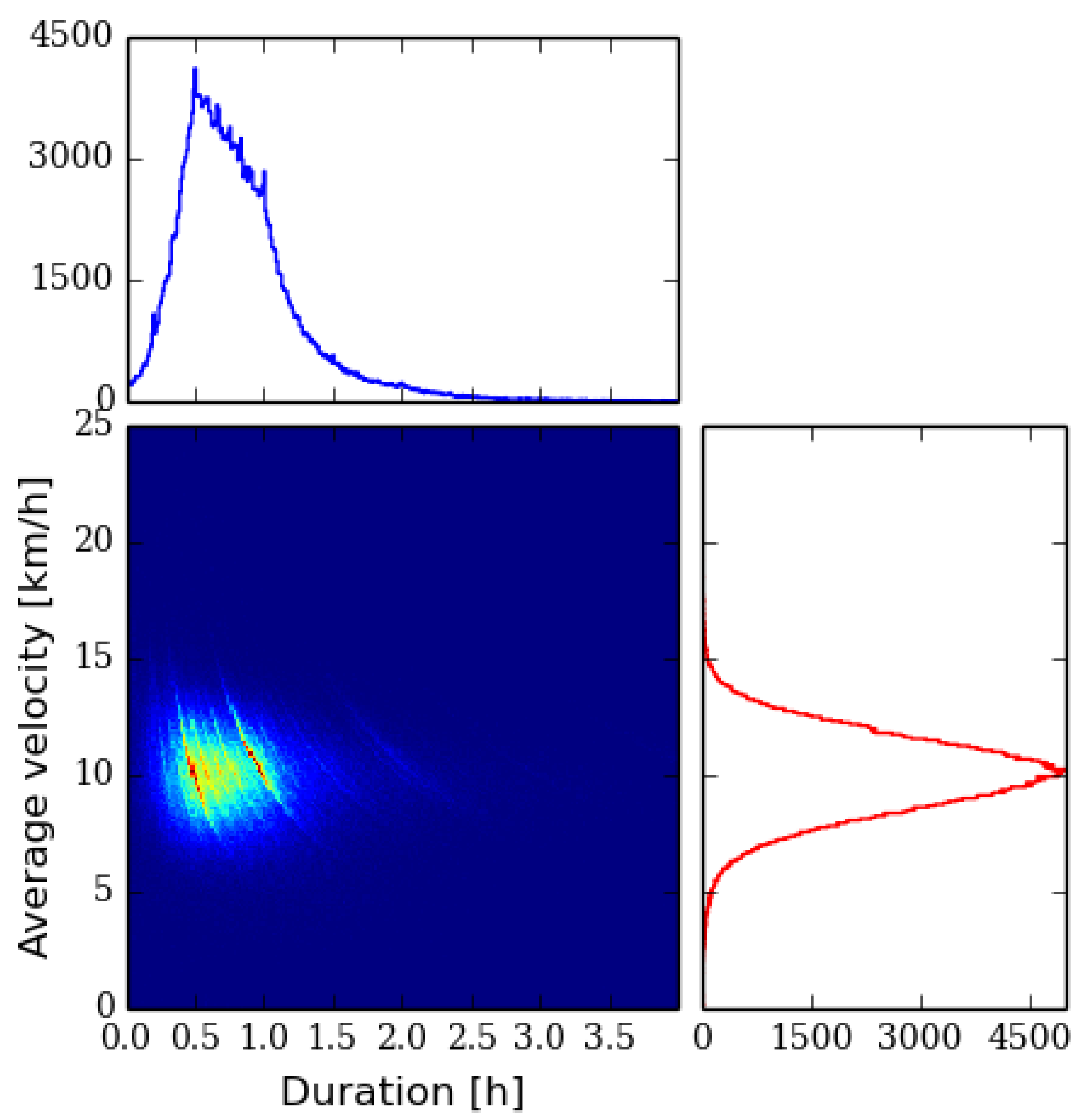
In Figure 1 we have plotted the histogram for all the 246,390 running tracks by 23,343 runners. A characteristic feature of the plot is the clearly detectable contour lines. They are caused by people running a constant distance with different durations, for example, in a competition. Popular city marathons are good examples of this kind of performances that are visible in the data. In the graph these correspond to curves $v_{\text{ave}}\Delta t=C$ where C is the constant total distance. Qualitatively the speed distribution looks Gaussian, whereas the duration histogram resembles an essentially log-normal distribution.

Figure 1. Histogram of the running tracks in terms of duration and average velocity with marginal histograms.

Figure 1. Histogram of the running tracks in terms of duration and average velocity with marginal histograms.

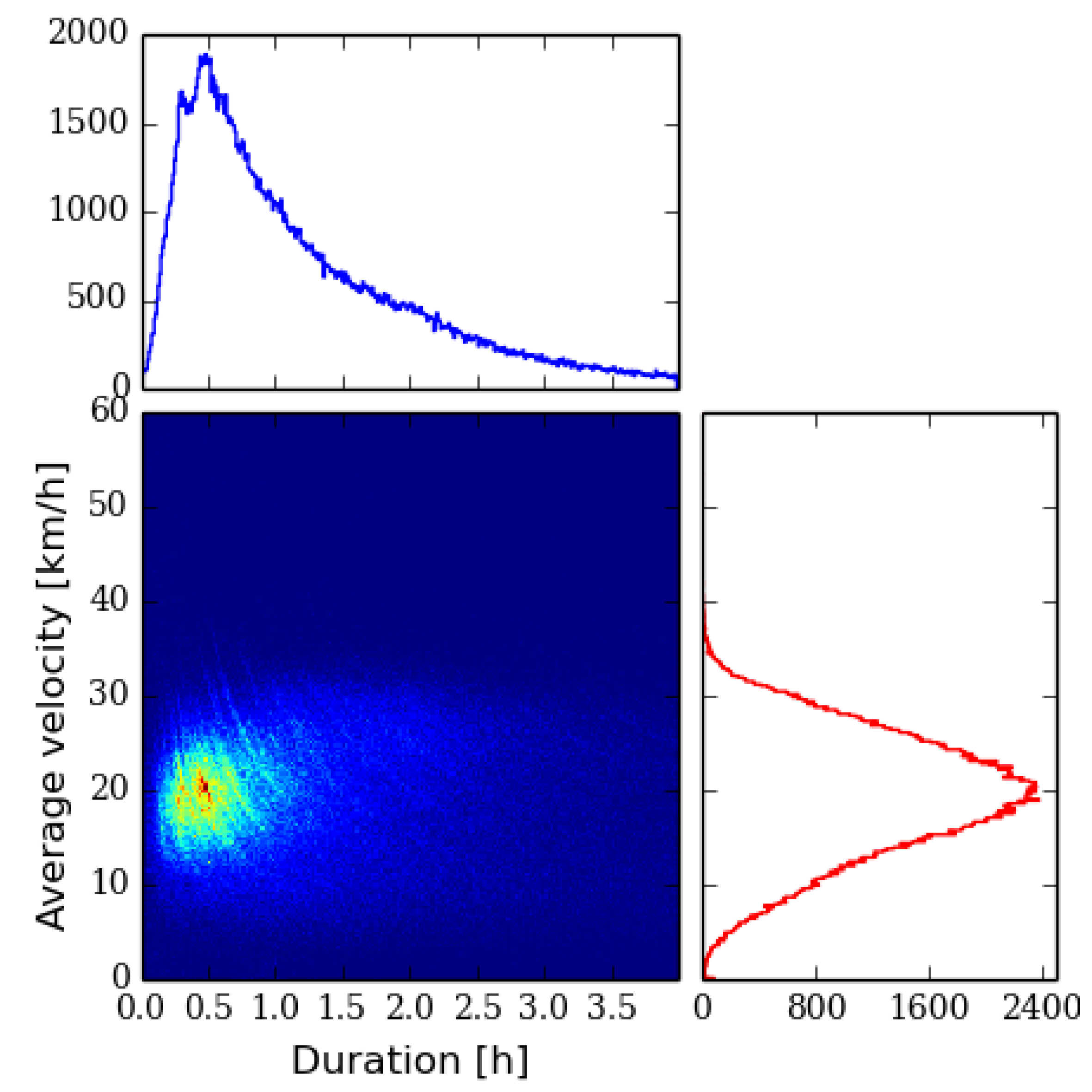
Figure 2. Histogram of cycling tracks in terms of duration and average velocity with marginal histograms.

Figure 2. Histogram of cycling tracks in terms of duration and average velocity with marginal histograms.

For the 149,784 cycling tracks by 18,163 cyclists the distribution in Figure 2 has features resembling the running track distribution. The main difference is that duration distribution has a longer tail with some of the performances lasting several hours. The presence of contour lines is not as distinctive as in the running data.

A separate question is whether our dataset is biased or non-biased as a sample representation of the running and cycling preferences of the total population. We argue that the heat map server designed and implemented in this work does not rely on this property at all. Instead, the heat map server will generate the heat maps irrespectively, and it will be up to the user to decide how the heat map should be interpreted and used.

4. Heat Map Generation

The objective is to generate heat maps that are displayed to the end-user using a map server. We assume that the background map is hosted by another server or has been generated beforehand and uses the Mercator projection [24] with a spherical Earth. We use a tile pyramid to save and display the created heat map with a tile size of 256 by 256 pixels. The program is written in C++ using the fastCGI library for communication with the Apache HTTP Server. We use a work queue and C++11 threads in the program and the mpm-worker in Apache to load balance the service request handling.

The efficient generation of heat maps requires much data preprocessing to reduce the amount of computation at request time. The Mercator projection depends on transcendental functions, which are computationally expensive. For 2.8 billion GPS points, this would lead to a significant time spent in the heat map generation and a noticeable lag in the web service. In addition, nearby GPS data points often map to the same pixel, leading to redundant calculations for the heat map. We decided to first preprocess all data by rasterizing the tracks, dividing them into zoom level tiles and sorting the data within the tiles. The preprocessed data can then be retrieved more efficiently to create heat maps.

4.1. Data Preprocessing

The spatial data is preprocessed by rasterizing every track and the rasterization is done using the pixels of the tiles. The major benefits are that the expensive Mercator projections are calculated offline and the size of the data is reduced significantly. The downside of this process is that information on the order in which the pixels were visited is lost. However, for this heat map service, this is non-critical. To optimize the calculation of the heat map, a rasterized track is not necessarily kept in one tile but is instead divided into segments based on the tiles that it overlaps. During the heat map generation, the program will quickly find all the track segments within a tile matching a query term and calculate the heat map from the results.

The key to quickly finding track segments matching an enduser’s query is to index the track data efficiently. We do this by using the tuple ($z,activity,Mortonindex$) as the index, where $Mortonindex$ is the Z-order or Morton value [25] of the tile coordinates at zoom level z. This is calculated by interleaving the binary representations of the coordinates. The data is sorted with respect to the index and thus track segments in a specific tile matching an activity can be found easily. In the preprocessing step we also gather the track segments from individual users with the same index value.

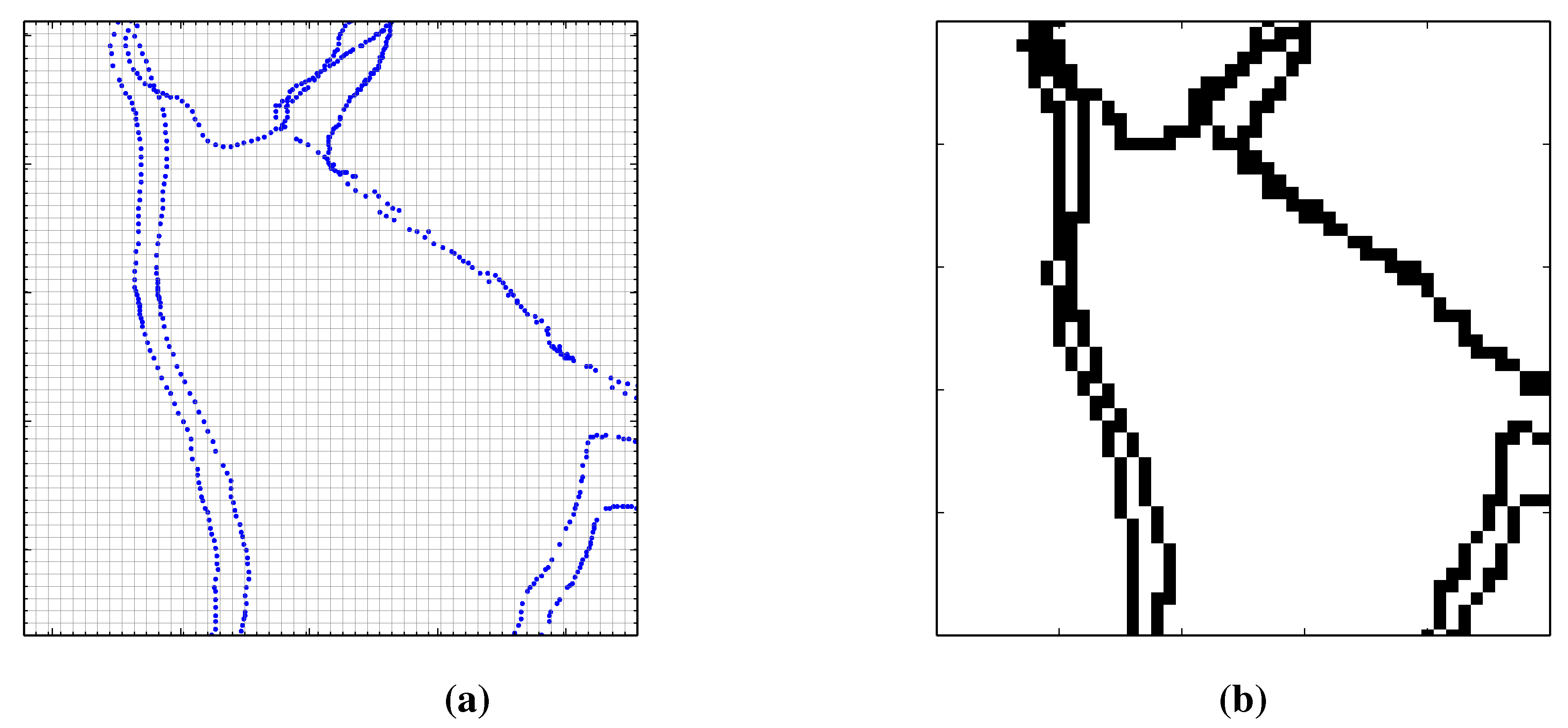
The user’s tracks are processed sequentially. A track is first rasterized at an initial zoom level and then divided into segments based on the tiles that intersect with it at this zoom level. The initial zoom level is set as 14, leading to a 9.55 m by 9.55 m pixel resolution. The GPS points of a sample track together with its lowest level Mercator grid is shown in Figure 3a and the corresponding rasterized track in Figure 3b. If a rasterized track is not continuous, that is, there are missing pixels in a path, Bresenham’s algorithm [26] is used to fill in the missing pixels. The pixels inside the 256 by 256 tiles are indexed using 16-bit integers and the unique values are stored in a C++ Standard Template Library (STL) vector. For this application we use Morton indices for the pixel coordinates within a tile, although a linear indexing with a stride equal to 256 could be used. The use of 16-bit integers allows us to lower the memory footprint. Tracks with the same tuple index value are appended to the same vector. Next the zoom level is decreased by one and the same rasterization procedure is done to the track. This process is continued until the lowest zoom level is reached for the heat map, which we have selected to be $z_{min}=3$. The end result is that user’s tracks have been pixelized at all zoom levels used in the heat map service. In order to estimate the number of raster points for a typical track at zoom level 14, we pick a typical track from Figure 2 obtaining a cycling track with the average speed of 20 km/h and the duration of 1 h. Assuming that one half of this track is spent going in a major compass direction generating $10,000/9.55\approx 1050$ pixels while the other half is in a minor compass direction covering $10,000/(9.55\times \sqrt{2})\approx 740$ pixels, we have in total 1800 pixels.

During the rasterization process we calculate some metadata related to a track that can be used to filter the tracks. These include the track length, the duration and the average velocity. We also store the number of local tile indices written into the STL vector for every track segment. Once a user’s tracks have been processed, the STL vectors with different tuple indices are combined into a single long STL vector, which we write to disk in a binary format. The tuple index together with the metadata for a track segment is written to a PostgreSQL server, which works as a long term storage for the data. PostgreSQL is also used to distribute the data to the server that calculates the heat maps. Since PostgreSQL servers can be pooled, these can be used to store much larger amounts of data than we currently have.

Figure 3. (a) Original track in blue are displayed together with the raster grid given by the Mercator projection at zoom level 14 with a tile size of 256 by 256 pixels. (b) The rasterized track that has been completed with Bresenham’s line drawing algorithm [26] to fill in any missing pixels.

Figure 3. (a) Original track in blue are displayed together with the raster grid given by the Mercator projection at zoom level 14 with a tile size of 256 by 256 pixels. (b) The rasterized track that has been completed with Bresenham’s line drawing algorithm [26] to fill in any missing pixels.

4.2. Map Creation

The end result of the preprocessing step is that all the filtered tracks have been rasterized and divided into tiles at the separate zoom levels. The relevant metadata of the tracks with the spatial indices of the tiles are stored in a PostgreSQL table. The heat map generation will essentially create fast queries to the database and visualize the results on the fly. Retrieving the results from PostgreSQL to C++, however, proved to be a performance bottleneck during program development. To improve the performance we read the metadata and the spatial index data from PostgreSQL to local memory and use that as a database. We use CUDA Thrust library [27] for storing and quickly accessing the data. The STL vectors are also read to memory from disk.

Database columns are stored to separate Thrust host vectors that are zipped together to create a key vector and a value vector. We use ($z,activity,Mortonindex,user\_id,track\_start$) tuples as the key with values given by ($month,track\_size$) tuples in the current implementation. Here the $user\_id$ variable is a unique integer ID assigned to all the hashed user IDs whereas the $track\_start$ and $track\_size$ terms are related to the binary files that were written in the preprocessing step: $track\_start$ gives the offset from the start of the file and $track\_size$ tells the program how many elements to read. The values are sorted by the key to enable the use of $thrust::lower\_bound$ and $thrust::upper\_bound$ functions to find track segments with specific values of z, $activity$ and $Mortonindex$.

The map creation starts with a request from the web client specifying the geographical area of interest, the zoom level, the activity type and possibly some other search criteria like the month of the year and/or the time of day. This is handled by the HTTP server (Apache HTTP Server in our case), which relays the request to the map creating daemon. It first checks whether the requested heat map tile already exists or needs to be created. A database request is parametrized in terms of the key tuple ($z,activity,Mortonindex,user\_id,track\_start$). Next the track segments with the matching values are found with the $thrust::lower\_bound$ and $thrust::upper\_bound$ functions. We then scan through these and filter the results based on the rest of the search criteria (currently month of the year, but this could easily be expanded). From those elements of the zipped vector that pass the filter we copy $user\_id$, $track\_start$ and $track\_size$ into new vectors. The user raster counts are calculated from these with Algorithm 1, where we essentially find all the unique pixels a user has visited in a tile and increment the corresponding values in a user count array. Once all users have been processed, for privacy we now zero pixels with user counts less than, say, five. The result is then written as a PNG image into a tile cache and finally sent to the web client. The largest user count values are most likely found in cities where the population size typically follows Zipf’s law or a power law [28]. We currently use a logarithmic scale for the pixel colors to cover the different orders of magnitudes of user counts more evenly. Another possibility is to use some local measure to highlight popular routes, for example, by calculating the distribution of user counts in a tile and its eight neighboring tiles and using a threshold value to color the pixels, e.g., Strava’s heat map currently uses a local coloring. The upside of this local coloring is that it shows locally popular routes more clearly and it is not sensitive to the size of the population of the city.

Algorithm 1: Calculation of the User Number Raster

1: input: arrays user, start, size 2: input: array inds                    ▹ user’s tile pixel indices 3: output: array counts                    ▹ user count buffer 4: function UserCount(user, start, size, inds, counts) 5:     tmp ← new array 6:     for each i do 7:         if user[i] = user[i+1] then 8:            for j ← start[i], start[i] + size[i] do 9:                insert inds[j] into tmp 10:            end for 11:         else                   ▹ next result is for a different user 12:            uniq = unique values in tmp 13:            for each id in uniq do 14:                counts[id] ← counts[id]+1 15:            end for 16:            clear tmp 17:         end if 18:     end for 19:  end function

5. Results

The server consists of an Ubuntu Linux system with a six core Intel Core i7-980 processor and 24 GB of main memory. The disk system uses a RAID-0 SSD drive for fast reads and writes. The map creating program uses 9.6 GB of memory of which 8.8 GB is used by the tile index data. The rest is used by the very simple database table scheme we are employing: putting all the data into one large table makes the queries easy to perform, but the track metadata is repeated several times for the segments of a track.

The most critical parameters for the server performance are the Apache HTTP server settings and the size of the thread pool that manages the tile requests. The Apache server uses mpm-worker, which is set to handle up to 6400 clients. The settings have been optimized for our application. For the thread pool we allocate 32 threads. A smaller number will increase the performance at lower numbers of users, but might cause timeout errors when thousands of clients request tiles simultaneously.

We have used the Apache JMeter application to stress test the heat map server. We simulate user behavior by randomly selecting a single tile $(x,y)$ at some zoom level z and then request the neighboring $5\times 5$ tiles using nested for loops. After the server returns, the user waits for a random time between 0 and 4 s that is sampled from uniform distribution and then requests another set of tiles. This behavior is meant to mimic an enduser making a request for one screen of tiles in a 5 by 5 grid and spending some time to view the returned heat map. All users repeat this 25 times during a simulation. The tile coordinates were limited to zoom level $z=14$ and to within southern Finland where the density of active Sports Tracker users is high. We ran the stress test on a four core Intel Core i7-3770K with 16 GB of main memory. Users were simulated using threads in the JMeter application and their number increases in powers of $\sqrt{2}$ (rounded to the nearest integer) during a test run. We study also the effect of the tile cache by enabling it in a second run and keeping the tiles created in the non-cached run on the RAID array.

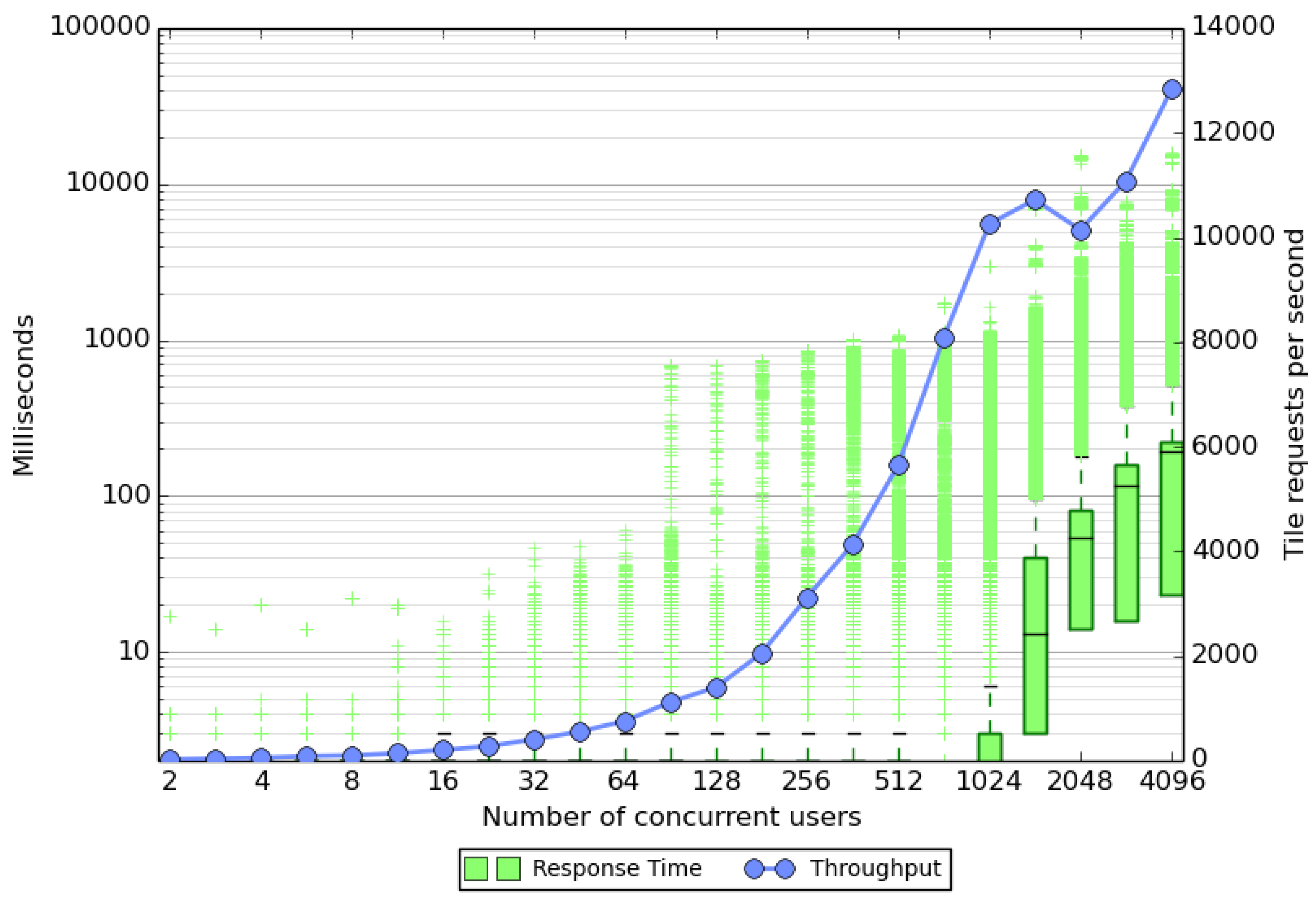
The stress test results with tile caching enabled are shown in Figure 4. The performance of the server is shown in terms of the response times and the throughput of the server. From the graphs it can be seen that the server can keep up fairly well with the requests up to around 2000 simulated users. At 1448 users only a few of the requests take more than two seconds to complete. However after this, the number of outliers grows, hence users may have to wait for several seconds for a reply in the worst case. This behavior naturally breaks the interactiveness of the service, at least for some of the users. The median response time, however, stays below 200 ms even at 4096 users. This behavior is most likely caused by the sparseness of the data. Many of the tiles do not have any GPS data available and these can be processed in a few milliseconds without the need to use Algorithm 1. The tiles with user data take roughly 25–40 ms to process when no other tiles are requested. When many of the requests are in these tiles, this can lead to queuing and long response times. The results from the throughput curve tell a similar story. At low user counts the server is not pushed to the limit and the server can provide more tiles than requested. Saturation occurs after 1024 users where the server can provide up to 12,000 tiles per second.

The results without the tile caching are shown in Figure 5. The response time is quite similar to the cached case, with the biggest difference being the slight increases in the outlier times at low user counts and in the median response times at high user counts. Accessing the heat map server during stress testing, however, seemed subjectively slower without the tile caching.

Figure 4. Stress test results for the server with tile caching. Note the logarithmic scale on the left axis. The green response time box gives the median time as a black line with the bottom and top of the box given by the first and third quartiles, respectively. Outliers are shown using a plus sign. The throughput is shown using a linear scale on the right. The stress testing did not cause any failed responses by the map server. The graph was created using a modified version of a python script [29].

Figure 4. Stress test results for the server with tile caching. Note the logarithmic scale on the left axis. The green response time box gives the median time as a black line with the bottom and top of the box given by the first and third quartiles, respectively. Outliers are shown using a plus sign. The throughput is shown using a linear scale on the right. The stress testing did not cause any failed responses by the map server. The graph was created using a modified version of a python script [29].

Figure 5. Stress test results for the server without caching. See Figure 4 for an explanation of the graph.

Figure 5. Stress test results for the server without caching. See Figure 4 for an explanation of the graph.

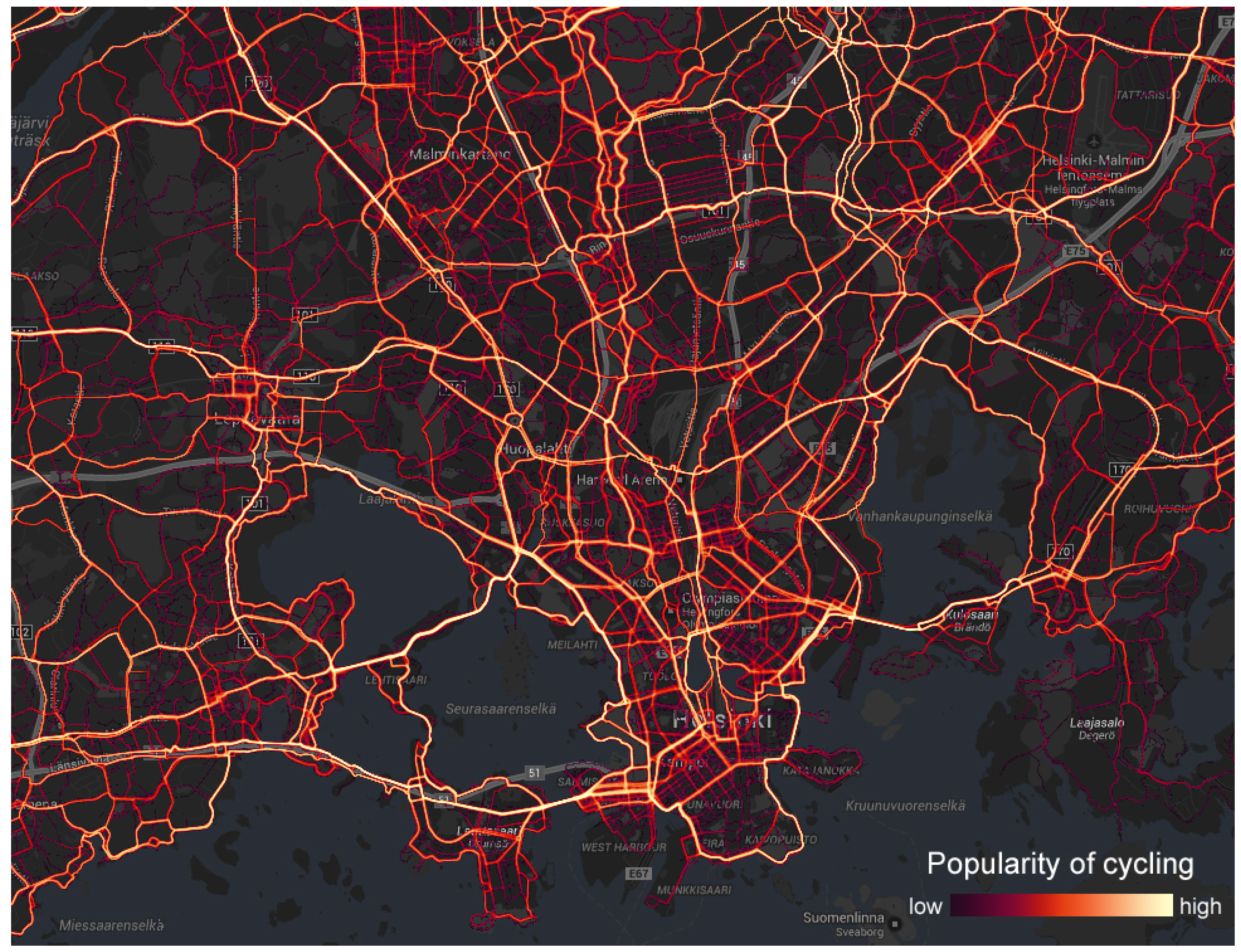
A sample heat map is shown in Figure 6 where we display popular cycling routes in the Helsinki region using a logarithmic scale. Bright yellow routes are the most popular ones, whereas purple routes are less popular. We require at least five different users in each pixel. If this criterion is not met the pixel is set transparent.

Figure 6. Heat map of popular cycling routes in Helsinki.

Figure 6. Heat map of popular cycling routes in Helsinki.

6. Conclusions and Future Work

We have presented an overview of an interactive server that provides heat map information on popular routes in sports. The overall design has been planned to make the tile creation as quickly as possible and to maximize the number of users that can access the server simultaneously. The performance tests indicate that even the current single node server can support over 1000 simultaneous users without significantly affecting the response time for the clients. Beyond this limit, the interactiveness requirement of the service can break down for some of the clients, but even then the median response time is less than 200 ms.

For larger data sizes and larger numbers of web clients, the server can either be replaced with a larger node, for instance a double socket Intel Xeon with more cores and memory, or scaled to a multiple node configuration. The metadata has already been prepared for this by storing it in a PostgreSQL server that can be scaled to several nodes. The heat map creation algorithm could be scaled with Message Passing Interface [30] to several nodes where the data is divided between the nodes. The design would have to be done carefully as the latency between the nodes might become a bottleneck. The location data could be also divided spatially into different regions that are processed in parallel. The HTTP server can be on a different node or distributed to several machines to scale up the performance.

The access logs from the heat map server can be further used in another data mining application to understand which regions and activities are the most interesting to the service users. The results could also be visualized in terms of heat maps [31] and used, for example, when load balancing the service.

References

- ITU. ICT Facts and Figures; International Telecommunication Union: Geneva, Switzerland, October 2014. [Google Scholar]
- Chittaranjan, G.; Blom, J.; Gatica-Perez, D. Mining large-scale smartphone data for personality studies. Pers. Ubiquitous Comput. 2013, 17, 433–450. [Google Scholar] [CrossRef]
- Gonzalez, M.C.; Hidalgo, C.A.; Barabasi, A.L. Understanding individual human mobility patterns. Nature 2008, 453, 779–782. [Google Scholar] [CrossRef] [PubMed]
- Herrera, J.C.; Work, D.B.; Herring, R.; Ban, X.; Jacobson, Q.; Bayen, A.M. Evaluation of traffic data obtained via GPS-enabled mobile phones: The mobile century field experiment. Transp. Res. Part C Emerg. Technol. 2010, 18, 568–583. [Google Scholar] [CrossRef]
- Ferster, C.J.; Coops, N.C. A review of earth observation using mobile personal communication devices. Comput. Geosci. 2013, 51, 339–349. [Google Scholar] [CrossRef]
- Nike Inc. Available online: http://nikeplus.nike.com/ (accessed on 15 September 2015).
- Sports Tracking Technologies Ltd. Available online: http://www.sports-tracker.com/ (accessed on 15 September 2015).
- Strava, Inc. Available online: http://www.strava.com/ (accessed on 15 September 2015).
- Chen, Z.; Shen, H.T.; Zhou, X.F. Discovering popular routes from trajectories. In Proceedings of the IEEE 27th International Conference on Data Engineering (ICDE), Hannover, Germany, 11–16 April 2011; pp. 900–911.
- Hood, J.; Sall, E.; Charlton, B. A GPS-based bicycle route choice model for San Francisco, California. Transp. Lett. Int. J. Transp. Res. 2011, 3, 63–75. [Google Scholar] [CrossRef]
- Liu, Y.; Wang, F.; Xiao, Y.; Gao, S. Urban land uses and traffic “source-sink areas”: Evidence from GPS-enabled taxi data in Shanghai. Landsc. Urban Plan. 2012, 106, 73–87. [Google Scholar] [CrossRef]
- Strava Inc. Heat Map. Available online: http://labs.strava.com/heatmap (accessed on 15 September 2015).
- Strava Inc. and Google Maps. Available online: http://engineering.strava.com/global-heatmap/ (accessed on 15 September 2015).
- Barkhuus, L.; Dey, A. Location-based services for mobile telephony: A study of users’ privacy concerns. In Proceedings of the 9th IFIP TC13 International Conference on Human-Computer Interaction, Zürich, Switzerland, 3–24 July 2003; pp. 709–712.
- Bonchi, F.; Lakshmanan, L.V.S.; Wang, H. Trajectory anonymity in publishing personal mobility data. SIGKDD Explor. 2011, 13, 30–42. [Google Scholar] [CrossRef]
- Apache JMeter. Available online: http://jmeter.apache.org/ (accessed on 15 September 2015).
- Long, J.A.; Nelson, T.A. A review of quantitative methods for movement data. Int. J. Geogr. Inf. Sci. 2013, 27, 292–318. [Google Scholar] [CrossRef]
- Silverman, B.W. Density Estimation for Statistics and Data Analysis; Chapman & Hall: London, UK, 1986. [Google Scholar]
- Oksanen, J.; Bergman, C.; Sainio, J.; Westerholm, J. Methods for deriving and calibrating privacy-preserving heat maps from mobile sports tracking application data. J. Transp. Geogr. 2014. [Google Scholar] [CrossRef]
- Lins, L.; Klosowski, J.T.; Scheidegger, C. Nanocubes for real-time exploration of spatiotemporal datasets. IEEE Trans. Vis. Comput. Graph. 2013, 19, 2456–2465. [Google Scholar] [CrossRef] [PubMed]
- Bär, H.R.; Hurni, L. Improved density estimation for the visualisation of Literary Spaces. Cartogr. J. 2011, 48, 309–316. [Google Scholar] [CrossRef]
- Sinnott, R.W. Virtues of the Haversine. Sky Telesc. 1984, 68, 159–163. [Google Scholar]
- The HDF Group. Hierarchical Data Format Version 5. Available online: http://www.hdfgroup.org/HDF5 (accessed on 4 March 2014).
- Maling, D.H. Coordinate Systems and Map Projections; Elsevier Science & Technology Books: Amsterdam, The Netherlands, 1992. [Google Scholar]
- Morton, G.M. A Computer Oriented Geodetic Data Base and a New Technique in File Sequencing; International Business Machines Company Ltd.: Ottawa, ON, Canada, 1966. [Google Scholar]
- Bresenham, J.E. Algorithm for computer control of a digital plotter. IBM Syst. J. 1965, 4, 25–30. [Google Scholar] [CrossRef]
- Hoberock, J.; Bell, N. Thrust: A Parallel Template Library. Available online: http://thrust.github.io/ (accessed on 4 March 2014).
- Gabaix, X. Zipf’s law for cities: An explanation. Q. J. Econ. 1999, 114, 739–767. [Google Scholar] [CrossRef]
- Metaltoad Load Tester. Available online: http://www.metaltoad.com/blog/plotting-your-load-test-jmeter/ (accessed on 15 September 2015).
- The MPI Forum. MPI: A Message Passing Interface. Available online: http://www.mpi-forum.org/ (accessed on 4 March 2014).
- Fisher, D. Hotmap: Looking at geographic attention. IEEE Trans. Vis. Comput. Graph. 2007, 13, 1184–1191. [Google Scholar] [CrossRef] [PubMed]
© 2015 by the authors; licensee MDPI, Basel, Switzerland. This article is an open access article distributed under the terms and conditions of the Creative Commons Attribution license (http://creativecommons.org/licenses/by/4.0/).