1. Introduction
Natural hazards can occur without warning and over a range of timescales. Therefore, the speed of onset and duration of hazardous events can vary considerably from the timescales of drought or global warming through to earthquakes, volcanoes or flash flooding. Humans can become susceptible to hazards for a variety of reasons contributing to voluntary and involuntary exposure such as societal attitudes [
1], economic constraints [
2], public policy [
3], collective memory [
4] and population growth [
5]. Globally, flooding is the most frequent natural disaster [
6]. Furthermore, the IPCC’s Fifth Assessment Report on climate change states with high confidence that there will continue to be an increase in economic losses and the number of people affected by flooding during the twenty-first century [
7]. Notable recent events in parts of northern Europe (Britain, Ireland and France), including a succession of intense winter storms in 2014, caused widespread flooding. While the flooding experienced in 2014 was not as severe as in previous years (e.g., 1947, 2007) economic losses in the UK and Ireland were still estimated to be US$1.5 billion [
8]. It was subsequently reported that the EA is reassessing English coastal flood risk as some maps may underestimate flood risk from coastal storm surges [
9]. This again demonstrated that it is not just one single extreme event that can lead to significant losses in both human and economic terms.
This paper aims to assess population exposure to flooding, as one exemplar hazard, through detailed local scale analysis of population movements. Populations are located in areas of relative hazard for a variety of complex reasons: whether resident as “inhabitants”, temporary occupants at places of work, study or leisure, or simply in transit through the region.
In order to better understand the risks posed to humans by hazard events, such as flooding, an improved knowledge of the spatial and temporal distribution of population is required [
10,
11,
12,
13]. Calculating population exposure is not straightforward as both the hazard and population vary over time [
14]. Inadequacies in mapping population have been noted for many decades [
15]. Commonly used official population datasets such as censuses or population registers usually provide only residential “night-time” population counts or at best simple “night-time” and “day-time” estimates. Better representations of population distributions that are time-specific are required for improved risk assessment and the development of effective emergency plans. Like hazard, population is not uniformly distributed across arbitrary zones. It is widely known that zonal population data are subject to the modifiable areal unit problem [
16], where the choice of areal units can have a greater impact than the phenomenon being observed.
Previous research applying high resolution spatiotemporal population modelling to assess exposure to natural hazards [
17,
18,
19], including flood risks [
20,
21], has shown large variations in population exposure over time and space. A major refinement in this approach, adopted by this paper, is the inclusion of seasonally varying overnight visitor population estimates developed by Newing
et al. [
22]. These have been integrated within the flexible Population 24/7 data framework [
23] which can be used to produce spatiotemporal gridded population estimates using variable kernel density estimation methods.
This paper demonstrates the analysis of seasonal variations in population exposure to flood risk in the town of St Austell, Cornwall in a coastal tourism area. It combines spatiotemporal population estimates with an extract from the UK’s national flood risk assessment and bespoke LISFLOOD-FP flood inundation modelling.
2. Case Study: St Austell, UK
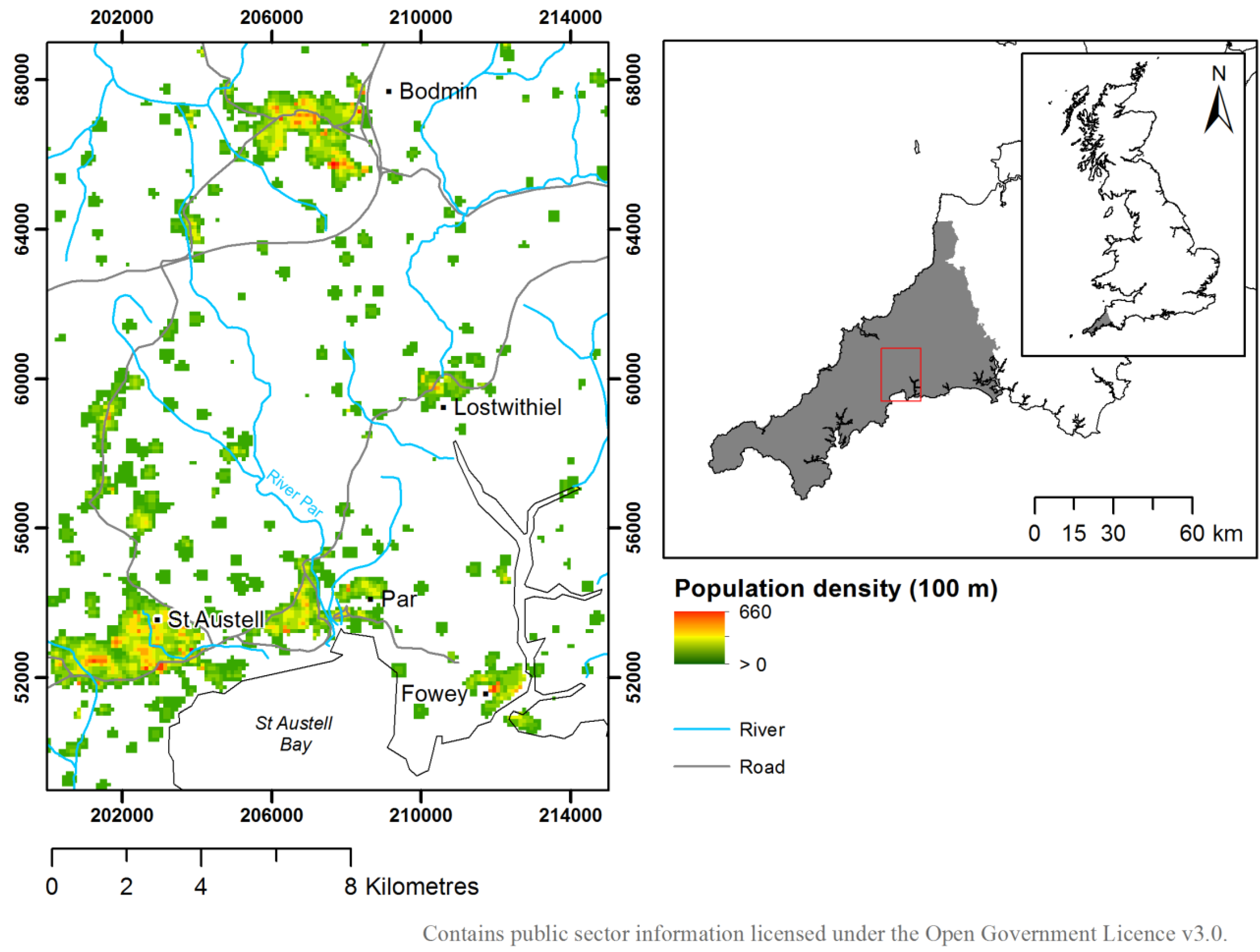
The assessment of seasonal population exposure to flood risk is demonstrated for a 15 × 20 km study area centred on St Austell Bay, Cornwall, UK (
Figure 1). It is located on part of the most southwesterly peninsula of Great Britain. St Austell is the largest town in Cornwall by population (19,958 2011 Census). The south of the study area is bounded by the coast along St Austell Bay and the Fowey estuary. Relatively small settlements are dispersed throughout pastoral farmland with the large expanse of Bodmin Moor to the northeast.
Local populations may fluctuate considerably on a seasonal basis, driven by an influx or outflow of students, seasonal workers and tourists at different times of the year [
24]. Within the UK many rural and coastal areas experience considerable seasonal influx of non-residential populations driven by tourism, especially during the peak summer season. The literature recognises that “tourists” or “visitors” are difficult to define, yet common definitions recognise that visitors are trip-making agents in an interaction process linking an origin and destination, whereby that destination is outside their usual environment and is visited temporarily for business or leisure purposes [
25,
26]. This broad definition covers a range of trips including day visits to attractions and overnight visits to friends and relatives, business travel and traditional conceptions of tourism representing “holidays”. Visitors are commonly segmented by their trip purpose and duration, with these characteristics recognised to have a clear impact on seasonal and spatial patterns [
27].
The southwest of England represents one of the most popular destinations for domestic tourism in the UK, with the county of Cornwall attracting around a quarter of all overnight visits to this region. Data from the United Kingdom Tourism Survey [
28] reveals the highly seasonal nature of domestic tourism in southwest England, with over 25% of visits classified as “Holiday 4+ nights” (in 2010) taking place during August. The southwest attracts almost 45% of domestic self-catered trips in England [
28] and over 35% of the highly seasonal camping and caravanning market (based on the number of trips) [
28]. Cornwall is home to a number of major resorts including Padstow, Bude, St Ives, Newquay and Fowey alongside major visitor attractions such as the Eden Project, one of the top 20 UK major paid attractions [
29] which attracts over a million visitors per year [
30]. Headline statistics such as these highlight the importance of tourism within destinations such as Cornwall, yet very little is known about visitor numbers or their seasonal and spatial distribution at the sub-regional or sub-district level. Coastal resorts in major tourist destinations such as Cornwall have enjoyed a recent period of growth in seasonal visitor numbers driven by the popularity of domestic holidaymaking [
31,
32]. Coastal resorts exhibit spatial clusters of accommodation, visitor facilities and attractions and thus experience considerable seasonal uplift in local non-residential populations. Visitors support the provision of local services and infrastructure which may not be viable based solely on the basis of residential populations [
33], but may also impact upon service delivery [
34,
35].
Figure 1.
St Austell study area outlined in red, showing location within Cornwall (shaded grey) and Great Britain insets. An example 100 m gridded population distribution provided for contextual purposes.
Figure 1.
St Austell study area outlined in red, showing location within Cornwall (shaded grey) and Great Britain insets. An example 100 m gridded population distribution provided for contextual purposes.
Coastal resorts within the study area, such as Par, Polkeris and Fowey, experience considerable seasonal fluctuations in population driven by an influx of domestic overnight visitors. The study area is also subject to fluvial, tidal and surface water flooding. The warning system on the River Par, within the study area, provides less than two hours’ notice of flooding [
36]. The “tide-locking” of local watercourses during high tides prevents drainage at coastal outlets and poses an additional risk of fluvial flooding. Tidal flood risk dominates the east of the study area. The Par area contains the highest number of properties at risk from current and predicted future flooding in Cornwall [
37].
3. Methods and Data
The method employed can be divided into three stages. Firstly, the spatiotemporal modelling concept is described and a model data library, comprising population datasets and temporal information, is outlined. Hourly population estimates at 100 m resolution have been produced for a “typical” weekday in January, May and August 2010 using the SurfaceBuilder247 software tool developed through the Population 24/7 project. These scenarios demonstrate the considerable variation experienced in estimated seasonal visitor numbers within the case study area, reflecting the low, fringe and peak tourist seasons respectively. Secondly, the construction of a seasonal visitor population dataset is reviewed and integrated into the spatiotemporal population modelling approach. Thirdly, bespoke flood inundation modelling is undertaken using LISFLOOD-FP to determine population exposure.
3.1. Spatiotemporal Population Modelling
The SurfaceBuilder247 software tool facilitates the creation of a gridded population surface estimate that is essentially dasymetric and volume preserving. It employs a variable kernel density estimation technique to redistribute the total population across space subject to a series of weights, constraints and temporal profiles. Residential population is redistributed from “origin” centroids, representing residential locations, to multiple classes of “destination” centroids. Classes of destination centroids are not exhaustive but include places of work, study, leisure, healthcare and retail. The redistribution of population to destination centroids is governed by a temporal profile specific to that activity class (e.g., school hours at a school site) and a known capacity for each centroid obtained from ancillary datasets. Further detail on the modelling framework and software is available separately [
23,
38,
39]. This paper demonstrates an example application.
A novel feature of this spatiotemporal modelling framework is the ability to handle the redistribution of user defined population subgroups independently. In this example, seven age subgroups corresponding to the population aged 0–3, 4–10, 11–15, 16–64 (students), 16–64 (non-students/working aged) and over 65 years were chosen. These age bands were selected because they have unique spatiotemporal characteristics relevant to the modelling undertaken. For example, school aged children are located at school sites during a term time weekday, and the working aged population at places of employment.
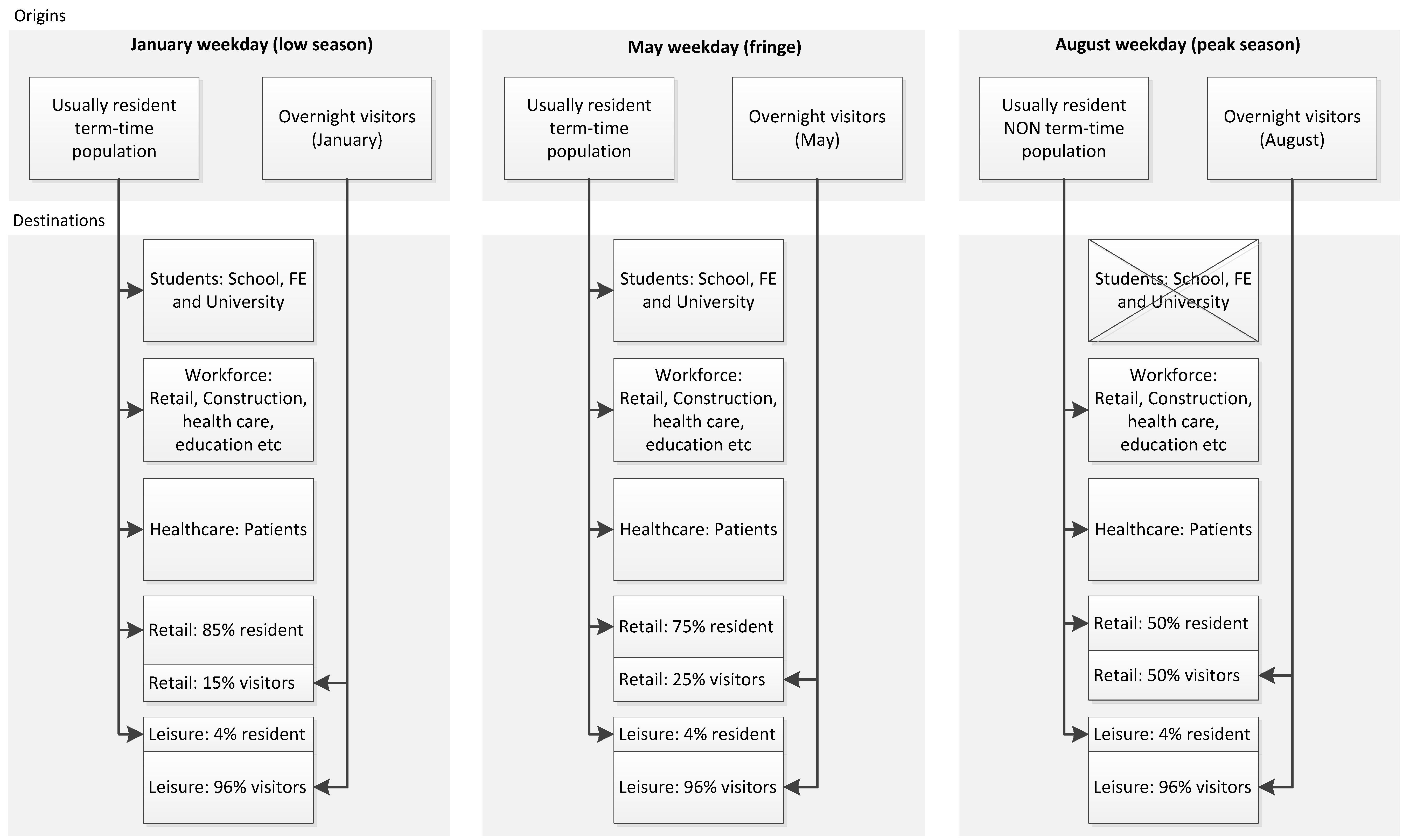
An overview of the model data library and the collection of origin and destination datasets constructed is provided in
Figure 2. The diagrammatic overview is outlined in two rows and three columns. Each column represents the seasonal scenario modelled. The first row concerns population origins and shows two different classes of origin which contain the usually resident and overnight visitor populations separately. The second row contains the destination locations. The connecting arrows show that different origin classes populate different (or different proportions of) destination locations. For example, the visitor population does not populate workplace or school destinations but is assigned to leisure destinations. A constant ratio of visitors (4%) to residents (96%) (
Figure 2) has been maintained for the leisure destinations. This is based on annual visitor origin data for county of Cornwall that are not reported sub-annually. Therefore, this provides a best estimate for composition and ensures that leisure destination demand is supplied from the correct corresponding origins (e.g., mostly visitors). However, while the ratio is constant the overall capacity, or expected footfall, of leisure destinations is not. It changes by season (
i.e., larger in August compared to January) therefore visitor and residential visits to these sites does increase seasonally. The seasonal change in visitor to resident retail footfall is informed by previous work by Newing
et al. [
22,
35] analysing loyalty card data for stores within this region.
Figure 2.
Diagrammatic overview of population origin and destination datasets used to construct the St Austell case study.
Figure 2.
Diagrammatic overview of population origin and destination datasets used to construct the St Austell case study.
The calculation of overnight visitors as a separate type of origin centroid dataset is described in the next section. Known counts of the “usually resident” population, the location where an individual spends the majority of their time [
40], are obtained from the 2010 mid-year estimate (MYE) for the study area. MYEs provide updated population estimates for intercensal years. This is used to create the origin destination dataset at the lower layer super output area (LSOA) level, the smallest geographical units for which MYEs are available (
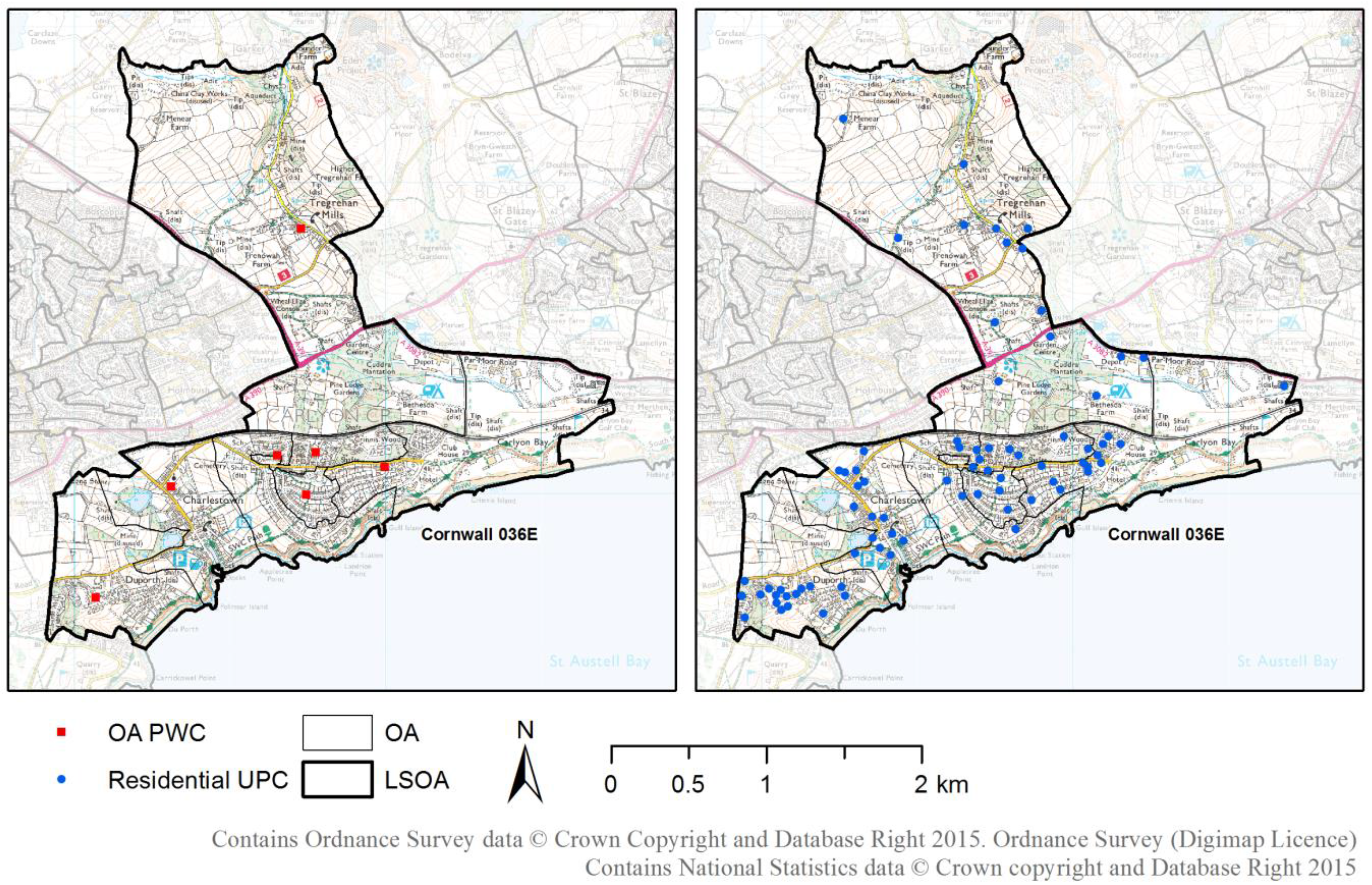
Figure 3). LSOAs are part of a hierarchical census structure in England and Wales for which population data are published. They represent around 1500 people and are further subdivided into OAs, the finest census unit available for England and Wales.
Figure 3 shows that the LSOA “Cornwall 036E” within the study area has seven constituent OAs, each with a corresponding population weighted centroid (PWC). LSOA 2010 MYEs were re-weighted onto residential unit postcodes (UPCs) by address count. UPCs are georeferenced points designed for the efficient delivery of mail and typically represent 15 residential addresses, or a single large user (business) [
41]. The use of UPCs as locations facilitates the accurate placement of population at inhabited locations and enables the detailed 100 m model output resolution achieved in this study. The use of UPCs is advantageous to using OA PWCs because of their improved distribution across inhabited locations (
Figure 3) despite the increase in computational demand. This improves accuracy in geographically larger LSOAs (e.g.,
Figure 3) where a greater areal extent in rural areas is required to maintain census confidentiality thresholds.
Figure 3.
An exemplar study area LSOA showing constituent OAs, OA PWCs and UPCs.
Figure 3.
An exemplar study area LSOA showing constituent OAs, OA PWCs and UPCs.
The expected population capacity of destination centroids (
Figure 2) was constructed from administrative, public and commercial datasets which are summarised in
Table 1. Where location data are not available within these datasets an individual site’s corresponding geo-referenced UPC was used.
Table 1.
Datasets used to construct destination centroids.
Table 1.
Datasets used to construct destination centroids.
| Destination Class | Dataset(s) | Data Attributes Used |
|---|
| Education | School Census 2010 | School enrollment figures |
| Independent Schools Census 2010 | School enrollment figures |
| Higher Education Statistics Agency (HESA) 2010 | Student enrollment figures |
| Workforce | Business Register and Employment Survey (BRES) 2010 | Employee count by LSOA by industry classification |
| Labour Force Survey 2010 | Work hours and shift types by industry |
| Healthcare | Hospital Episode Statistics 2010 | Patient (in/out/A&E) count by provider |
| Retail | GMAP 2010 | Retail centre locations and floor space |
| Company annual performance data | Sales per unit floor area (£/sq. ft.) |
| Leisure | VisitEngland 2010 | Regional visitor origins for Cornwall |
| Association of Leading Visitor Attractions | Attraction annual visitor numbers |
| National Travel Survey 2010 | Distance travelled for daytrips |
| English Heritage 2010 | Monthly distribution of visitor numbers (Cornwall) |
3.2. Seasonal Population Fluctuation
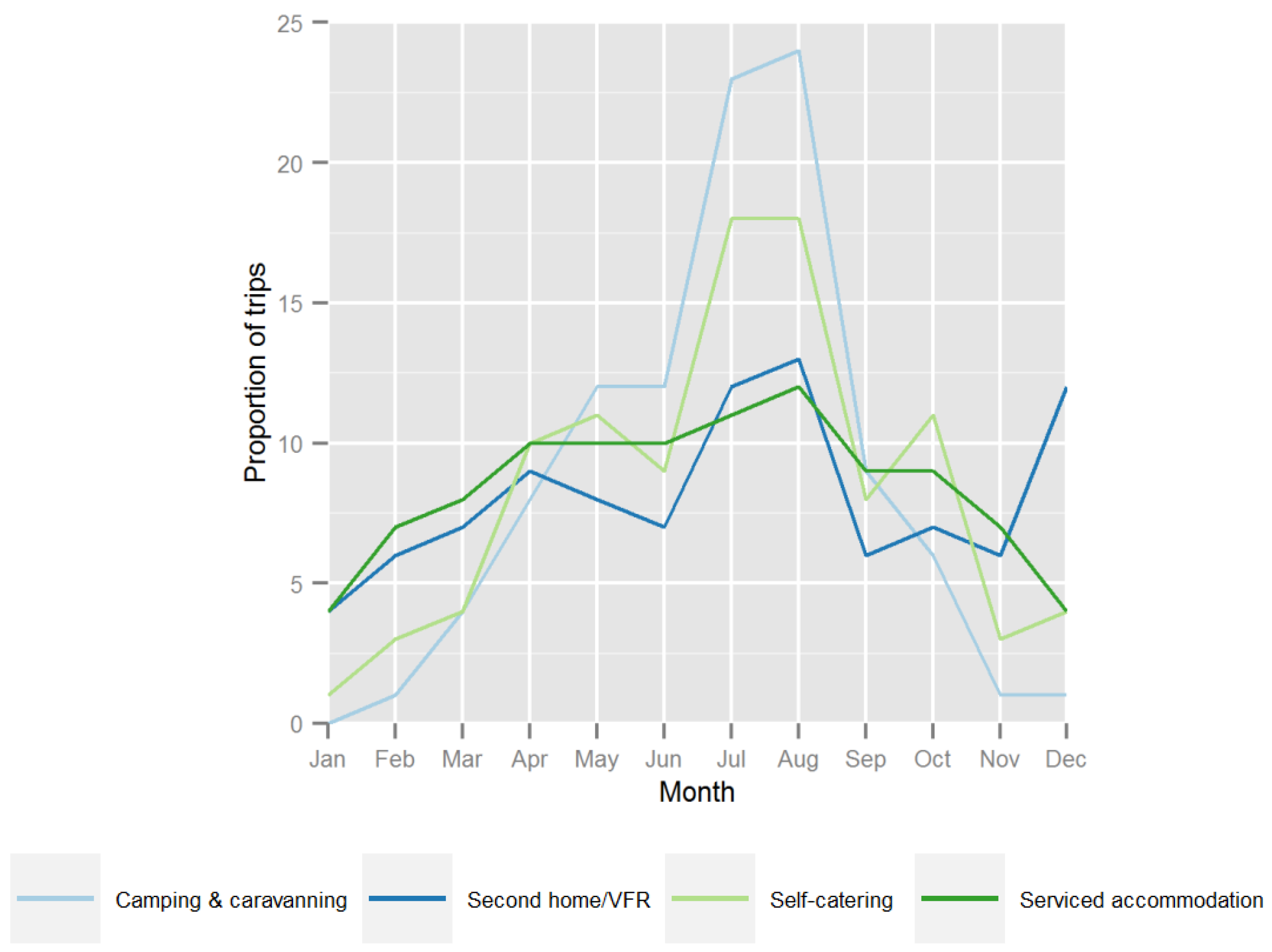
The seasonal distribution of (domestic) trips by accommodation type is shown in
Figure 4. Self-catering accommodation, and in particular camping and caravanning (shown separately), exhibit a very pronounced seasonal pattern with almost a quarter of all camping and caravanning trips beginning during August (with a further 23% in July). Many forms of self-catered accommodation (such as accommodation located on holiday parks) tend to exhibit a high degree of spatial clustering. This results from the concentration of a large number of accommodation units on large sites alongside provision of visitor facilities (such as entertainment and swimming pools). Not only does this produce considerable spatial clusters of visitors, these may be highly seasonal, driven not only by the school calendar and national holidays, but also by the operating season at these establishments. It is not possible to discern these trends from static decadal census estimates making them inappropriate for flood risk assessments.
Tourist visitor populations have a tendency to cluster in both space and time. In coastal areas, such as St Austell Bay, a concentration of visitor accommodation, attractions and other facilities generate spatial clusters of visitors, with numbers known to fluctuate at different times of the year, driven by the weather, local and national events, the institutional calendar and the operating season at accommodation sites and major attractions. In contrast to residential and workplace populations, very little is known about the spatial or temporal distribution of overnight visitors below the local authority district level.
Figure 4.
Seasonal trip distribution (all domestic trips) based on accommodation type. Constructed using UK Travel Survey Data [
28].
Figure 4.
Seasonal trip distribution (all domestic trips) based on accommodation type. Constructed using UK Travel Survey Data [
28].
We make use of a novel dataset estimating the seasonal and spatial distribution of overnight visitors (
Table 2). These estimates account for all visitors staying overnight within the study area (domestic and international tourists) and were built from the “bottom-up”, taking individual accommodation “units” as the building block, aggregated to the unit postcode or census Output Area (OA) level to form visitor “origins”, as outlined fully in Newing
et al. [
35]. Accommodation units may represent commercial accommodation (e.g., a hotel room, self-catering cottage or camping pitch), or be drawn from the existing housing stock (holiday/second home, or home of a hosting friend or relative). Commercial accommodation was derived from a comprehensive database provided by South West Tourism (SWT) and covering all accommodation known to SWT (via audits) in the county of Cornwall at the end of the year 2010 and was cleaned, validated and updated prior to use. After validation, each accommodation site (in the case of hotels, campsites
etc.) or unit (in the case of individually rented cottages
etc.) was geo referenced by its unit postcode and associated with a capacity (number of bed-spaces), forming the commercial accommodation stock. Actual visitor numbers will be driven by the accommodation stock in conjunction with occupancy rates which form an established indicator of accommodation utilisation within the tourist sector. To generate our estimates, accommodation stock (by type) within each unit postcode has been multiplied by its respective occupancy rate (at different times of the year) to identify likely “occupied units”. These are then “populated” based on surveyed data related to party sizes and age breakdown, by accommodation type, drawn from the most up to date survey of visitors in this destination, at the time of writing [
42].
Table 2.
Overnight visitor estimates within the St Austell study area.
Table 2.
Overnight visitor estimates within the St Austell study area.
| Month (Season) | Overnight Visitor Count |
|---|
| January 2010 (Low) | 1,000 |
| May 2010 (Fringe) | 6,300 |
| August 2010 (Peak) | 12,400 |
Visitors staying with friends and relatives (VFR) and those using second/holiday homes do not have a clearly identifiable “stock” of accommodation (counts of second homes were not routinely part of small-area data collection at the time of modelling, but information on these dwelling was collected for the first time as part of the 2011 census). Cornwall Council provided some limited information on overall numbers of second home units at a middle layer super output area (MSOA) level based on data collected through council tax records in 2008, and these were resampled across the unit postcodes making up the study area, with assumptions made about utilization rates based on limited anecdotal evidence available. Similarly, estimating the number or spatial distribution of visitors staying with friends and relatives is tricky since this form of accommodation is routinely overlooked and may not follow the seasonal peaks or spatial distribution of other forms of accommodation, yet represent an important driver of tourist populations. The “stock” of accommodation that can be used for VFR visits is theoretically all existing residential households. Unlike commercial accommodation, it is not possible to build from the “bottom-up” (
i.e., identify stock and then apply utilisation rates). Instead a “top-down” approach is required, whereby the estimated total number of VFR “nights” countywide (4.09m) [
29] were distributed temporally and spatially across the possible stock of host households, assuming that every domestic dwelling is a potential host and that all households host the same number of overnight visits, using United Kingdom Tourism Survey (UKTS) data to identify the temporal distribution across the year [
28] and broken down by surveyed age distributions. Whilst major holiday parks and camping and caravanning sites generate spatial and temporal clusters of overnight visitor populations in areas which may have few or no usual residents, VFR and second home tourism generates considerable volumes of overnight visitors, but far lower incidences of noticeable spatial clusters. The characteristics of domestic trip-making behaviors were used to determine the seasonal distribution of visits. However, these estimates of small area visitor populations (counts) do incorporate international visitors, since the process to populate accommodation units with visitors does not discriminate between visitors by origin. Characteristics of domestic visits are used to determine the seasonal distribution of visits as the literature and Great Britain Tourism Survey (formerly UKTS) recognise the importance of domestic tourism in driving tourism trends in South West England (see also [
25]).
In common with the approach used for residential populations, visitor populations are redistributed from their overnight origins to daytime locations such as major attractions, the transport network and leisure locations which may not traditionally be thought of as clusters of population in the same way as workplaces, hospitals and retail centres. Given the coastal and estuarine nature of the study area, some of these locations may also be at flood risk. Considerable effort was required here in order to identify tourist origins and to assign capacity and utilisation constraints. The visitor accommodation sector is highly fragmented (lots of small providers with ease of entry and exit). As such, no comprehensive database of visitor accommodation exists, yet many organizations, including local destination marketing organizations (DMOs) such as “VisitCornwall” hold partial information about accommodation they actively market or have quality assessed. We benefitted from access to a database held by “South West Tourism”, representing the most comprehensive listing of accommodation available for this study area, at the time of writing. Nevertheless, considerable additional updating and data cleansing was required. For application in alternative study areas, the effort required and subsequent accuracy of visitor “origins” would be dependent on the quality of local data collection related to the accommodation stock.
3.3. Flood Inundation Modelling (LISFLOOD-FP)
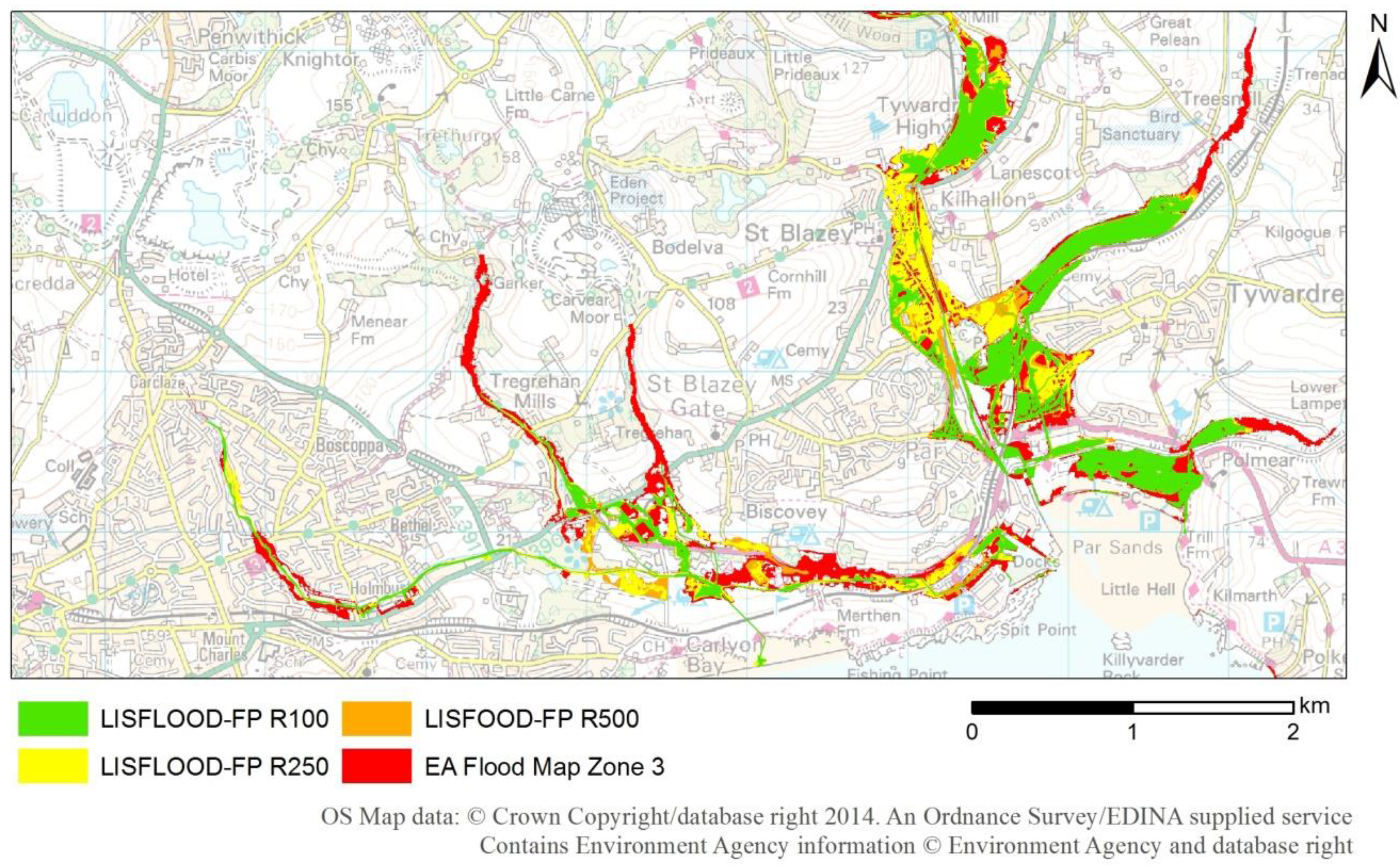
Three flood scenarios representing return periods (R) of 100, 250 and 500 years have been created using LISFLOOD-FP [
43], a two-dimensional raster based flood inundation model, for an 8 × 4 km subsection of the study area (
Figure 5). The return period represents the likelihood of an event of a given magnitude occurring based on an 11 hour rainfall event. In addition, the Environment Agency’s (EA) flood map zone three (FMZ3) represents the amalgamation of return periods for events of 100 (fluvial) and 200 (tidal) years. FMZ3 contains a greater extent for a comparable lesser magnitude, however bespoke LISFLOOD-FP outputs specifically account for defences and other structures, also providing an estimate of flood depth and velocity (enabling a better estimation of the resulting hazard relative to extent alone). The presence of flood defences and effect of buildings is not accounted for, and only flood extent is recorded in FMZ3.
Figure 5.
Comparison of LISFLOOD-FP and Environment Agency flood inundation for the selected area covering St Austell and Par within the study area.
Figure 5.
Comparison of LISFLOOD-FP and Environment Agency flood inundation for the selected area covering St Austell and Par within the study area.
In contrast to the static EA flood map (
Figure 5), bespoke modelling of the individual characteristics of the precise area concerned provides the potential to support more detailed analysis and scrutiny. The LISFLOOD-FP model DEM was constructed from bare earth (2 m resolution) LiDAR surveys obtained from the Environment Agency [
44]. Raster LISFLOOD-FP flood extents were produced with a 5 m output resolution. It has been suggested that at least a 5 m resolution is essential for modelling flow dynamics within urban areas to account for small scale variations [
45]. Buildings were subsequently rasterised and added to the DEM based on OS MasterMap data [
46,
47] layers in order to explicitly represent the blocking effect upon propagating flood waters. The river network (and information relating to flood defences where available) was obtained via the Environmental Agency. River widths were approximated manually using Google Earth imagery.
The river network was split into sub-sections within which depths were estimated based on return period capacities, accounting, where possible, for defence return standards. As the region is largely ungauged, the Flood Estimation Handbook software [
45] was used to provide flow time series estimates for rainfall events of varying magnitudes, which were then used to estimate river depths and floodplain inundation throughout the domain. For instance, undefended river reaches were assumed to have flow capacities of approximately 1 in 2 year return periods, while defended reaches capacities were specified in the defence data information where available (typically 1 in 50 years within the UK). LISFLOOD-FP is an appropriate model for this application because it is both computationally efficient at high resolution (1–10 m) and the code can be run on the latest high performance computing technology [
48]. However, a wide selection of research and commercial two-dimensional hydraulic models could be applied to get similar outcomes. Three raster layers corresponding to the three pluvial event return periods of 100, 250 and 500 years, each with an ocean boundary condition representing a 1 in 200 year water level [
49], were loosely-coupled with population outputs from SurfaceBuilder247. The LISFLOOD-FP outputs were vectorised and population exposure for each scenario calculated using zonal statistics in ArcGIS. All layers have been combined with seasonally varying population estimates to analyse the effect of spatiotemporal cycles. The EA Flood Map has also been included here because it is the currently accepted national flood hazard map used by planners and local authorities.
4. Results and Discussion
It has already been noted that results at this spatiotemporal scale are not achievable when coupling traditional population data with information on hazards. The selected study area is geographically constrained by the coastline and largely rural in nature. However, the study area notably experiences a large flux of visitors on a seasonal scale. For this reason, and in part due to the rural nature, daily commuter flows do not dominate this example. Instead, different temporal factors on a larger seasonal scale are the primary influences on this region.
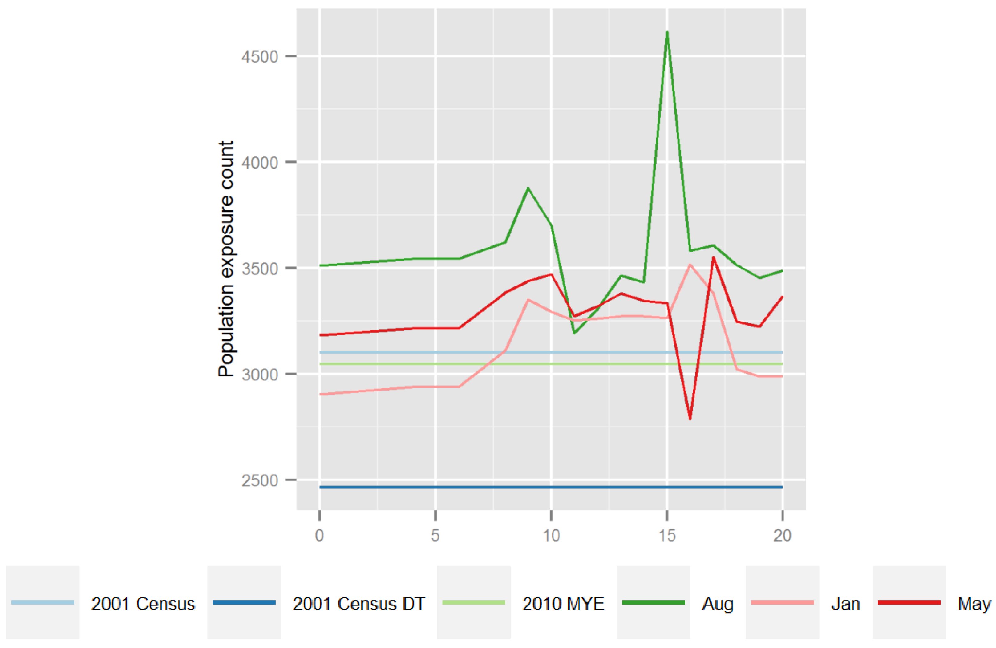
Figure 6 shows hourly population exposure to FMZ3 for the whole study area representing a “typical” working weekday. Modelled outputs have been compared with static exposure estimates from rasterised census outputs representing: the baseline 2001 Census population at OA level (highest resolution available), 2001 Census daytime population at OA (only available for 2001) and the 2010 MYE (closest to target date but only available at the LSOA level). In comparison to the static census data time-specific population estimates provide a much greater insight to exposure to flood hazard. Large peaks (e.g., August,
Figure 6) become more pronounced as a result of high-intensity population clustering driven by seasonal visitor fluctuations. The change of magnitude represented within this sample of results alone illustrates major implications on flood risk analyses which are shown to depend on time of the day and season of the year.
Figure 6.
Flood exposure estimates from the Environment Agency Flood Map Zone 3 for the St Austell study area using census and seasonal spatiotemporal model outputs at hourly intervals for a “typical” weekday.
Figure 6.
Flood exposure estimates from the Environment Agency Flood Map Zone 3 for the St Austell study area using census and seasonal spatiotemporal model outputs at hourly intervals for a “typical” weekday.
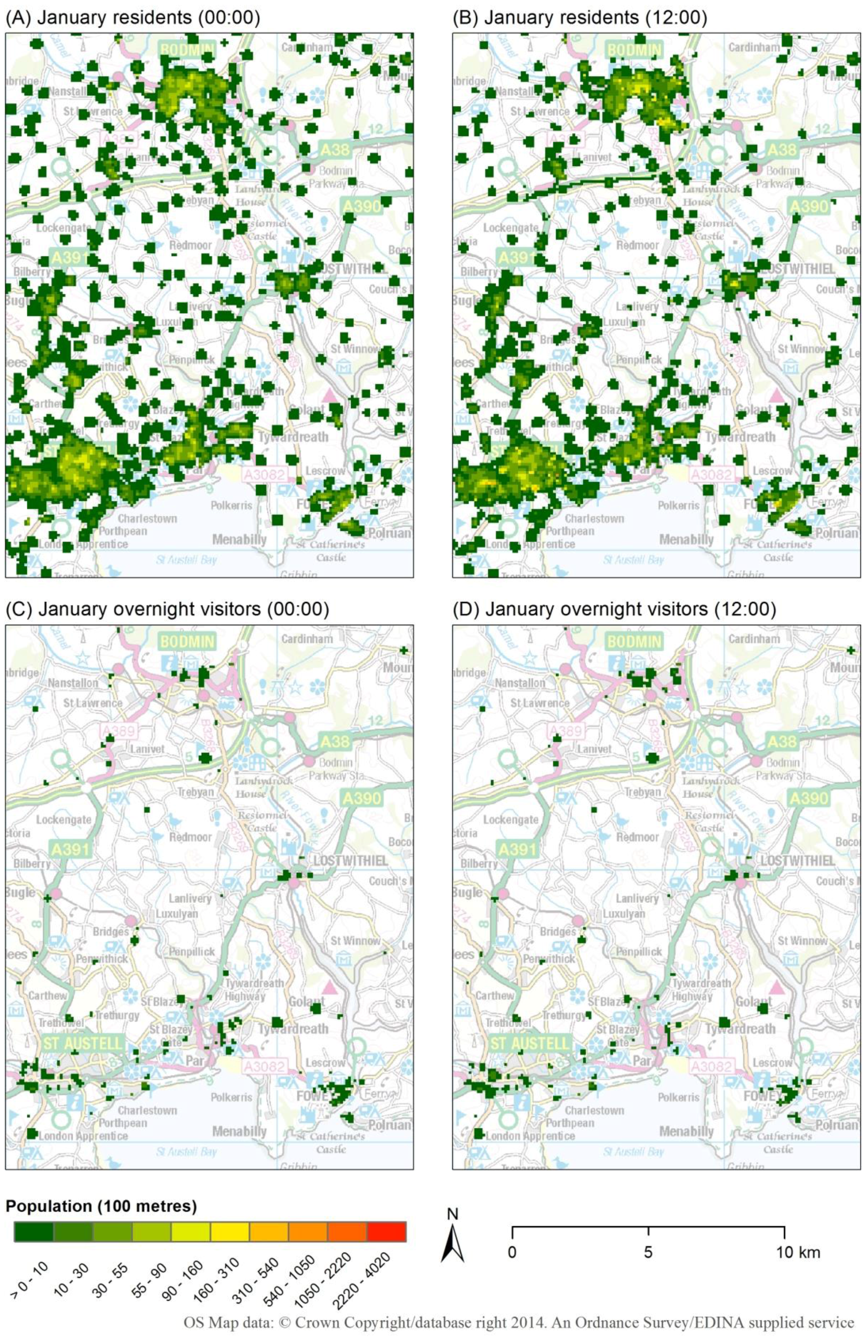
Seasonal spatiotemporal population variation has been illustrated for a weekday day-time (12:00) and night-time population (00:00) estimate for the January (low season) and August (peak season) scenarios modelled. The usually resident and overnight visitors have been displayed separately (
Figure 7 and
Figure 8). In both examples a general concentration in the usually resident day-time (12:00) population occurs from the night-time (00:00) locations. Increased clustering at the main population centres can be observed in the day-time examples (St Austell to the south and Bodmin in the north) and a greater population in travel on the road network. The concentration is observed in the main population centres, analogous with the workplace locations showing rural-urban commuter flow from the surrounding areas by the usually resident population. For example, for the August usually resident population there is a peak in concentration in the St Austell town centre at 12:00 (
Figure 8B) of 2200 people/100 m
2, compared to just 55 people/100 m
2 at 00:00. This is represented at the group of red coloured cells in the south-western corner of the study area in
Figure 8B. It also highlights the known phenomenon that town centres are predominantly only populated during the daytime as they host a range of retail, leisure and workplace locations but at night have a minimal usually resident population.
Figure 7.
Modelled seasonal population distribution (100 m) for the St Austell study area for a January weekday. (A) usually resident night-time (00:00) population, (B) usually resident daytime (12:00) population, (C) overnight visitor night-time (00:00) population and (D) overnight visitor daytime (12:00) population.
Figure 8.
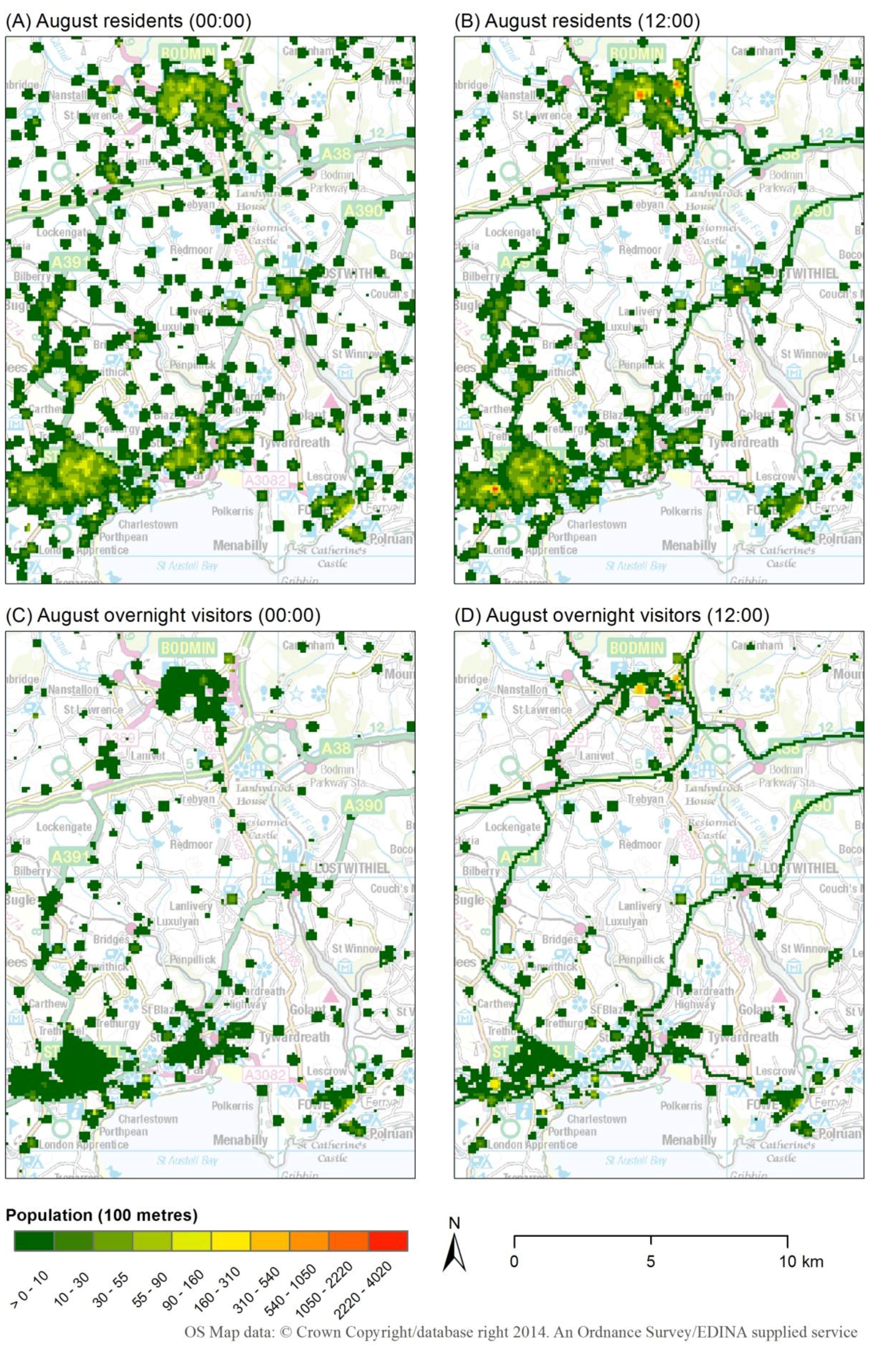
Modelled seasonal population distribution (100 m) for the St Austell study area for a August weekday. (A) usually resident night-time (00:00) population, (B) usually resident daytime (12:00) population, (C) overnight visitor night-time (00:00) population and (D) overnight visitor daytime (12:00) population.
Figure 8.
Modelled seasonal population distribution (100 m) for the St Austell study area for a August weekday. (A) usually resident night-time (00:00) population, (B) usually resident daytime (12:00) population, (C) overnight visitor night-time (00:00) population and (D) overnight visitor daytime (12:00) population.
Figure 9.
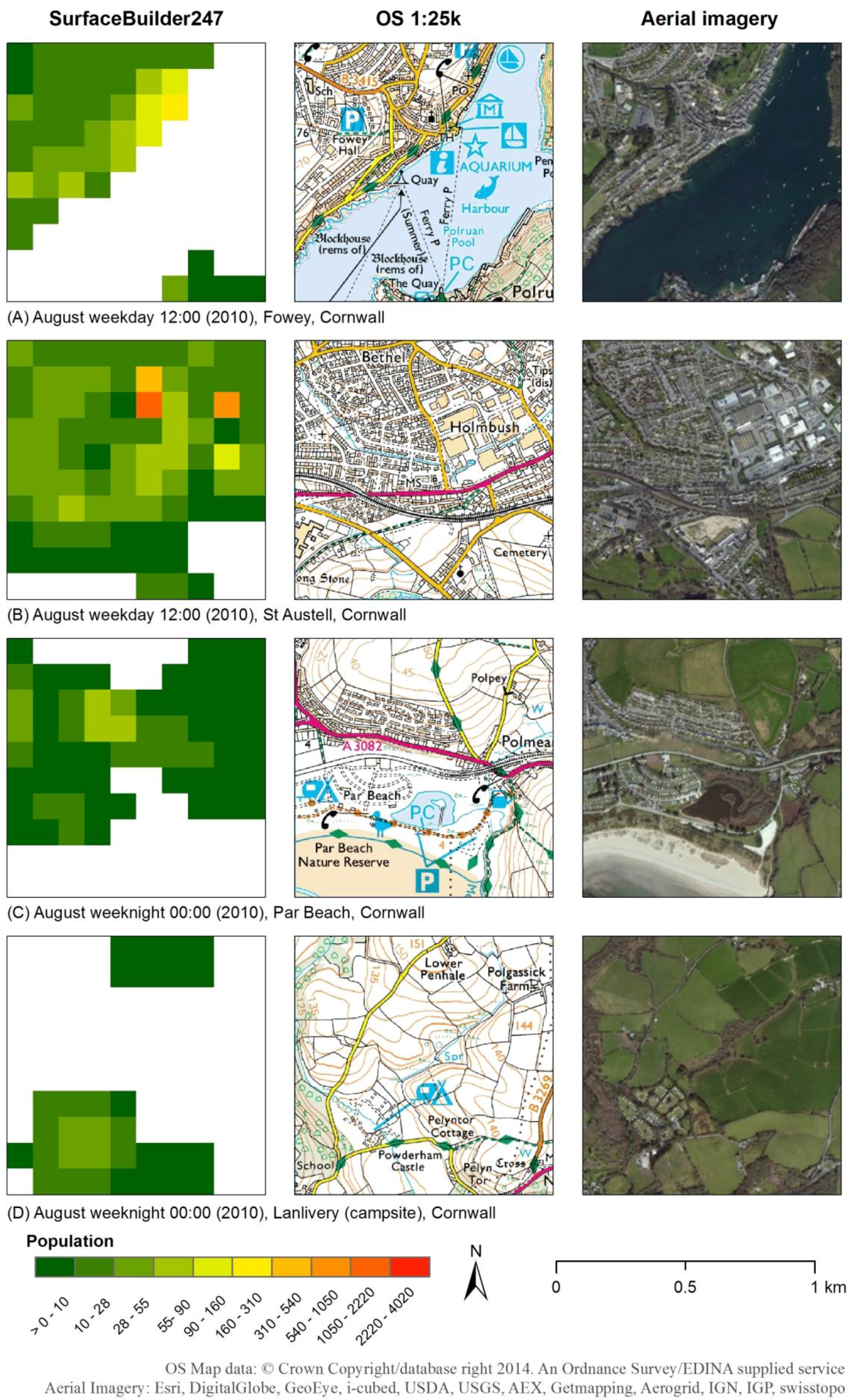
A detailed comparison of SurfaceBuilder247 (100 metre resolution) results within the St Austell study area with 1:25,000 scale OS background mapping and aerial imagery for selected 1 km national grid squares. (A,B) August weekday “daytime” population. (C,D) August weekday “night-time” population.
Figure 9.
A detailed comparison of SurfaceBuilder247 (100 metre resolution) results within the St Austell study area with 1:25,000 scale OS background mapping and aerial imagery for selected 1 km national grid squares. (A,B) August weekday “daytime” population. (C,D) August weekday “night-time” population.
Similarly, there is a concentration in the overnight visitor population from the night-time locations they occupy to concentrated locations of daytime activity (
Figure 7 and
Figure 8C,D). These daytime concentrations, most notable in August with the visitor peak, occur in the main town centres (e.g., St Austell, Bodmin and Lostwithiel). Overall, there is a large increase in the overnight visitor population of greater than 11,000 people between January and August (
Table 2). Another clear observation is that the distribution as well as concentration and number of estimated overnight visitors increase between January and August. Most notable is the August night-time concentration of visitors in the coastal areas south of St Austell (
Figure 7C). Secondly, the central area of the study area’s extent receives a greater share of overnight visitors. This is attributed to the location of rural guesthouses, campsites and caravan parks which are not shown as populated within traditional census datasets.
A detailed comparison has been conducted using selected 1 km national grid square extracts from the St Austell study area model results (
Figure 9). Two examples have been selected from the August daytime (
Figure 9A,B) scenario and two for an August night-time (
Figure 9C,D). All represent the total population (usually resident and visitors combined). The distribution of 100 m output cells is visible within the 1 km square extracts. The modelled results have been compared to Ordnance Survey (OS) base mapping and aerial imagery for the same location and scale for contextualisation.
The OS map extract for the first example (
Figure 9A) shows part of Fowey, with a range of tourist attractions (indicated by the blue map symbology). The August daytime model results for the same area show that the population is appropriately constrained to the land mass (due to the background masking layer) and concentrated on the coastal locations of the amenities outlined on the map extract.
The second extract is focused on one of the highest concentrations within the study area (
Figure 9B), showing part of St Austell town centre. The August daytime population concentration exceeds 1000 people. The Holmbush area is a retail district which includes a large shopping complex. St Austell has the greatest floor space in terms of retail within the study area which is informed by the retail destination datasets that have been created for this case study. Comparison with the aerial imagery shows close model alignment with populated areas.
The third (
Figure 9C) shows the location of a large static caravan site immediately behind Par Beach. Population densities within the model cells correspond with the caravan site, summing to approximately 150 people. The aerial imagery provides the detail which is just shown as a series of tracks on the OS background mapping (as caravans are not permanent structures and therefore not mapped). This area also corresponds to high levels of flood risk under all of the inundation scenarios (
Figure 5).
Finally, the fourth extract (
Figure 9D) illustrates the night-time population estimate for what appears to be an uninhabited area, but which is clearly designated as a campsite in the OS mapping and discernible within aerial imagery. The population density corresponding to the campsite area shows moderate population densities of up to 50 people per 100 m
2 during peak season. The small settlement of Lower Penhale is represented by an area of low non-zero population densities. This appears to be a slight overspread, but still demonstrates a refinement based on the census zonal data alone. Furthermore it would not be possible to resolve the August peak in population at this campsite (which is simply an unoccupied field at other times of the year) relying on census data alone. This example tests the limits of the current spatial resolution of the model using available population data for this case study; however they are still significant improvements. Reasons for this overspread are likely to be caused by the underlying population origin centroid density. As residential postcodes were used the rural locations identified on the map, Lower Penhale and Polgassick Farm (
Figure 9D) are likely to share a postcode which may not be georeferenced directly on one particular site. The dispersed nature of rural properties sharing a postcode is greater than in concentrated streets in urban areas. This is another important factor to consider in the application of models using only postcode centroids where spatial accuracy and density can vary.
Daytime seasonal population flood exposure estimates corresponding to the inundation extents illustrated in
Figure 5 are provided in
Table 3. These relate to the EA’s flood map zone three (FMZ3) and 100, 250 and 500 year LISFLOOD-FP (L-FP) scenarios. There is a general trend in population exposure as anticipated with increasing geographic inundation extent and concentrated seasonal visitor population estimates. An interesting phenomenon observed in this seasonal flood map analysis (
Table 3) is the decrease in the August 12:00 exposure to the LISFLOOD-FP R100 flood scenario, compared to the May 12:00 exposure total to the same LISFLOOD-FP R100 flood extent. Total (visitor and usually resident) population exposure for a “typical” weekday at 12:00 under the LISFLOOD-FP R100 scenario decreases from 580 to 563 from May to August. This is driven by the usually resident population. It is the reverse of the cycle observed in all of the other scenarios modelled where the August 12:00 residential population exposure increases relative to the respective January and May levels. The midday January and May exposure of the usual residents for the LISFLOOD-FP R100 scenario remain similar. This is expected as they are derived from the same term time census population base. The August usually resident population base accounts for non-term time population but nonetheless this is still an increase in population so not a cause for the decrease in exposure..
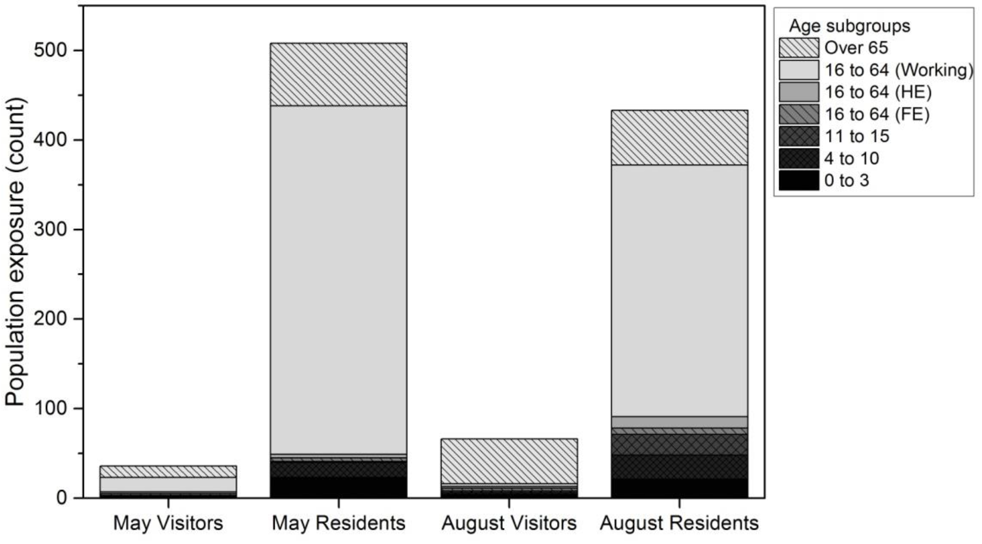
To examine the unexpected decline in flood risk exposure for the August and May LISFLOOD-FP R100 scenario (
Table 3) the population has been further analysed at the population subgroup level for seven age subgroups for both usual residents and visitors (
Figure 10). It can be observed that the largest contribution in the decline in exposure to flood risk between May and August (at 12:00 for LISFLOOD-FP R100) is the 16–64 working aged population. Exposure in this group decreases from 389 to 281 between May and August. This may be unexpected as it could be anticipated that total exposure increases by season in line with population. However, this phenomenon highlights the effect of the chosen time (weekday midday population estimate) and flood polygon areal extent.
Table 3.
Daytime usually resident and visitor population exposure to three LISFLOOD-FP inundation scenarios (R = return period) and EA flood map zone three for January, May and August (increasing levels of inundation left to right).
Table 3.
Daytime usually resident and visitor population exposure to three LISFLOOD-FP inundation scenarios (R = return period) and EA flood map zone three for January, May and August (increasing levels of inundation left to right).
| Population | L-FP R100 | L-FP R250 | L-FP R500 | FMZ3 |
|---|
| Residents 12:00 Jan | 542 | 939 | 1069 | 1725 |
| Visitors 12:00 Jan | 2 | 5 | 7 | 15 |
| Total | 544 | 944 | 1076 | 1740 |
| Residents 12:00 May | 546 | 994 | 1139 | 1729 |
| Visitors 12:00 May | 34 | 108 | 131 | 114 |
| Total | 580 | 1102 | 1270 | 1843 |
| Residents 12:00 Aug | 498 | 1019 | 1178 | 1741 |
| Visitors 12:00 Aug | 65 | 206 | 249 | 212 |
| Total | 563 | 1225 | 1427 | 1953 |
Figure 10.
Comparison of daytime (12:00) population LISFLOOD-FP R100 exposure estimates broken down into age subgroups for visitors and residents in May and August.
Figure 10.
Comparison of daytime (12:00) population LISFLOOD-FP R100 exposure estimates broken down into age subgroups for visitors and residents in May and August.
Although the total population exposure to flood risk in August for LISFLOOD-FP R100 decreases compared to May, the number of the elderly (>65 years) potentially exposed increases (
Figure 10). This increase of 385% (May to August) is derived from the influx of overnight visitors. While overall it would appear that flood risk is lower, there is actually a large increase in the elderly population exposed to flooding in the R100 August weekday 12:00 scenario. This does not mean that overall elderly visitors dominate the whole study area’s August tourist population (also dominated by family holidays) but just the flood polygon analysed. This insight could not be achieved looking at the total population alone or without modelling exposure at population subgroup level. While overall flood exposure did not increase in this example, this approach identified a significant increase within the proportion of an elderly vulnerable subgroup.
The SurfaceBuilder247 approach facilitates detailed evaluations for population exposure to flood risk while considering changes in season and time of day. In any final assessment there is the potential for large variations in the outcome depending on the combination of events chosen, as exemplified in this St Austell application.
It is not yet possible to fully and independently validate the population analyses undertaken. However, a high confidence should be placed on the models construction from known population counts at specific locations. These are based on rigorous administrative datasets and associated with quantifiable population flows. Censuses are typically utilised for validation opportunities, but the approach presented here significantly moves beyond static census estimates. Some national censuses are published at high spatial resolution (100 m) grid format (e.g., Austria [
50]), but still remain static, primarily residential, counts. Increasing prevalence of social media and mobile telephony data analysis may provide future opportunities to advance the work presented here further or point towards a potential validation mechanism [
51,
52].


 ,
, 


