Article

The Spatiotemporal Dynamics of Forest–Heathland Communities over 60 Years in Fontainebleau, France

1
Centre d'Ecologie et des Sciences de la Conservation (CESCO, UMR7204), Sorbonne University, MNHN, CNRS, UPMC, CP51, 55 rue Buffon, Paris 75005, France
2
EA 2219, UFR Sciences et Techniques, University of Western Brittany, 6, Avenue Victor Le Gorgeu, CS93 837, Brest 29238, France
3
Museum National d'Histoire Naturelle, CNRS UMR MNHN 7179, Mécanismes Adaptatifs: des Organismes aux Communautés, 1 Avenue du Petit Château, Brunoy 91800, France
*
Author to whom correspondence should be addressed.
ISPRS Int. J. Geo-Inf. 2015, 4(2), 957-973; https://doi.org/10.3390/ijgi4020957
Submission received: 14 November 2014 / Accepted: 12 May 2015 / Published: 3 June 2015
(This article belongs to the Special Issue Spatial Analysis for Environmental Applications)

Abstract

:
According to the EU Habitats Directive, heathlands are “natural habitats of community interest”. Heathland management aims at conserving these habitats threatened by various changes, including successional processes leading to forest vegetation. We investigate the dynamics of woody species to the detriment of heathland over a period of 60 years in the Fontainebleau forest and we examine the effects of soil types, soil depth and topography parameters on heathland stability. We assess changes in forest cover between 1946 and 2003 by comparing vegetation maps derived from aerial photographs coupled to GIS analyses. The results show the loss of more than 75% of heathland during 1946–2003 due to tree colonisation of abandoned heathland. We detected differences in the dynamics of colonisation between coniferous and deciduous trees. The colonisation of heathland by coniferous species was faster over the last 20 years of our study period. Tree encroachment was faster in north-facing areas and in areas of acidic luvisols. While this dynamic was very slow in acid sandstone soils, heathland stability was more important in shallow soils on flat and south facing areas. Our study has the potential to assist land managers in selecting those heathland areas that will be easier to conserve and/or to restore by focusing on areas and spatial conditions that prevent forest colonisation and hence favour the long-term stability of heathland.

1. Introduction

Global changes threaten natural ecosystems that are collapsing and even completely disappearing [1]. Their conservation is a priority in order to halt biodiversity loss [2] and is currently assured by conventions and programs that aim at maintaining and restoring natural habitats. Different management methods must be used to keep threatened habitats in a favourable state of conservation [3], such as controlling natural succession and the physical structure of the vegetation, to preserve species or species assemblages of conservation concern [4]. European heathland habitat is a typical example of a habitat where such active management is required. European heathlands are dominated by a characteristic plant species, Calluna vulgaris (L.) Hull, [5], which is a main resource for specialist species of birds and invertebrates [6,7]. This habitat is restricted to nutrient-poor, acidic soils [8], and is a pioneer stage in natural succession [9] except when heathlands occur naturally in some coastal areas. The large areas of European heathlands all over North-Western Europe were maintained by traditional agro-pastoral practises over the last 3000 years. Since agricultural intensification occurred in the 1950s, these traditional land uses have almost completely disappeared. As a result, heathland areas have been drastically reduced because vegetation on nutrient-poor, acidic soils has been overrun by woody species. Since the designation of ericaceous heathland in Annex I of the E.C. Habitats Directive 1992 as a type of natural habitat of community interest, habitat management plans are increasingly aimed at preserving heathland species and habitats [10] and keeping them in a favourable state of conservation. Nevertheless, many studies show woodland expansion in the heathland despite the application of different measures to maintain this habitat, such as prescribed burning and mechanical cuttings [11]. Under the prevailing circumstances of climate change and nitrogen deposition, the conservation of heathland becomes more difficult and requires more intensive management practices [12] at increased cost [13], because drought and the seasonal precipitation changes influence the competitive balance between species. On the other hand, the increase of nitrogen deposition rates in terrestrial ecosystems improves soil fertility and the competitive ability of grasses, but to the detriment of heathland [14,15].
In this context, identifying the influence of spatial variability in soil and topography on forest heathland mosaic dynamics becomes a real necessity in order to determine the most appropriate management methods for the long-term conservation of this mosaic. The dynamics of plant communities are directly associated with soil type variability, as soil mineral resources are a structuring factor for the organisation of vegetation [16]. Indeed, spatial variation in physiographic factors can also control vegetation [17,18,19] and plant populations [20], which could influence the dynamics of the forest to the detriment of the heathland.
In the Fontainebleau forest 50 km south from Paris, France, heathland is still present as small patches embedded in more woody areas, forming a very complex mosaic-landscape hosting particular species. In this forest, the presence of acid sandy soils and the traditional agro-pastoralism had favoured the establishment and maintenance of the heathland over thousands of years. The abandonment of ancestral land uses since the second half of the 20th century has caused a decline of heathland. At present, 1400 ha of heathland remain, in fragmented patches embedded in an oak-pine forest integrated within a Managed Biological Reserve. Since the early nineties, the National Forest Office (ONF), following French obligations in relation to EU Directives, has attempted to preserve many patches of heathland by regularly cutting new plantlets of woody species. This maintenance is becoming more and more difficult due to the spatial configuration of the many heathland fragments, which are interspersed within a large matrix of conifer and deciduous forests. The most economical management methods, such as regular mechanical cuttings and woody species removal, are inadequate to maintain specific species in a heathland fragment in the middle of a forest matrix as we showed in previous studies [11,21]. These conditions require additional methods to better preserve this habitat.
In the present study, we use spatio-temporal analysis based on aerial photographs to describe changes in the forest heathland mosaic over a period of 60 years in order to understand the recolonisation processes of forest trees on abandoned heathland. In this study we also sought to assess the influence of soil properties (soil type and depth) and physiographic factors (slope and aspect) on driving land cover changes in this area.

2. Materials and Methods
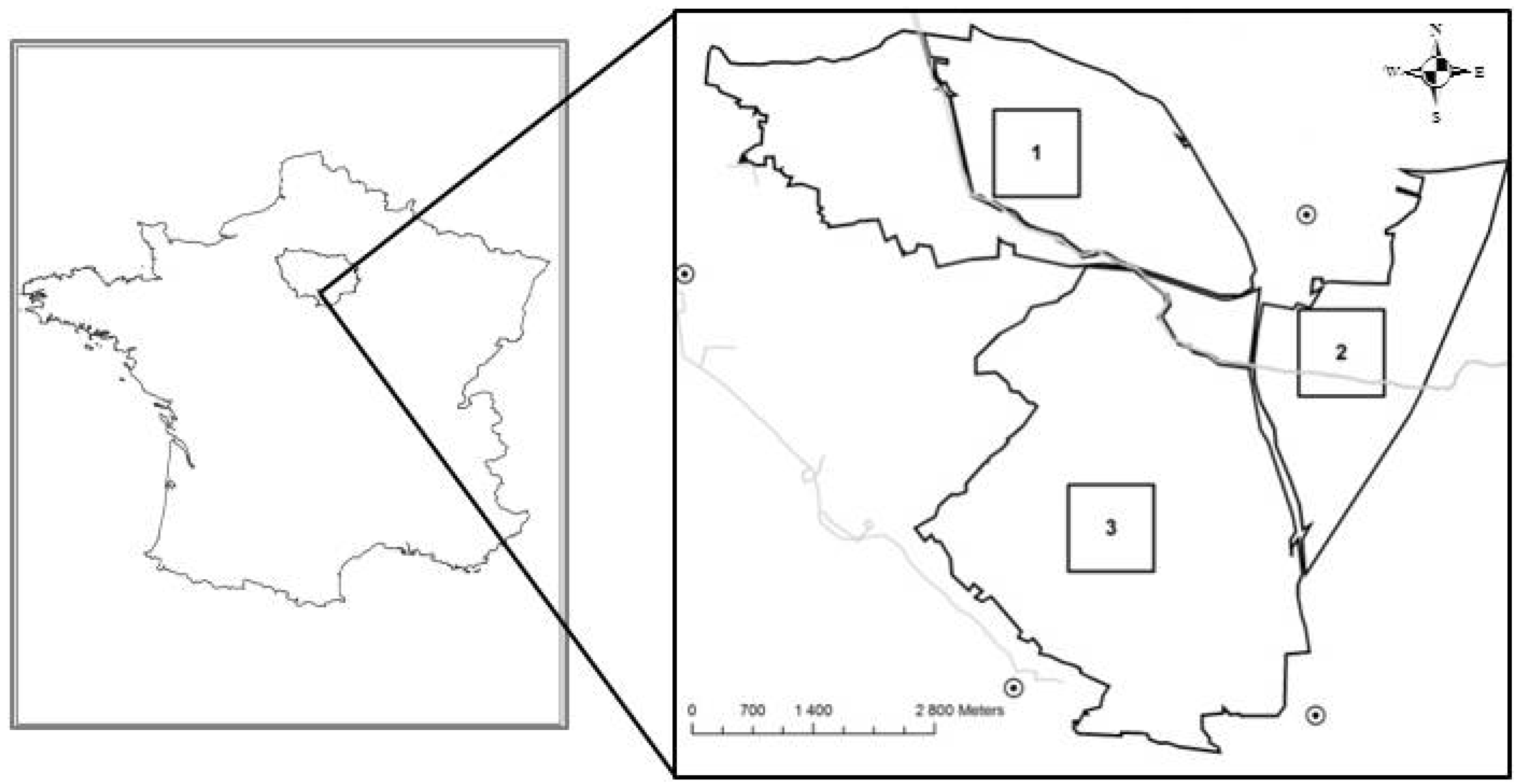
2.1. Study Site

The state-owned forest called the “Trois Pignons”, with 3307 ha, is part of the Fontainebleau Forest (Figure 1), and consists of a mosaic of heathland and forest: 83 ha of managed heathland and approximately 540 ha of heathland with less than 10% woody cover are embedded in a matrix of conifer and deciduous forest. We selected three field sites of 1 km2 each, characterised by recolonisation of the heathland by the forest. Each site is at a different stage in the heathland-forest dynamics, knowing that the heathland was present at the three sites in 1946; the sites also vary in terms of the ecological conditions. The first site is the Mares aux Joncs (“Ma”), which is a Stampian landscape with sandstone outcrops that create hyper-acidic hydromorphic environments. The second site, Chanfroy (“Ch”), is a low plain with a mixture of silica sands and limestone gravels, while site 3 is Cul du Chien (“Cl”), another Stampian landscape comprised by pure silica sands and hyper-acidic.
Figure 1. Location of the three study sites in the (Trois Pignons) forest: 1. Mares aux Joncs (Ma), 2. Chanfroy (Ch), and 3. Cul du Chien (Cl). The grey lines represent rivers and dark dots represent cities.
Ijgi 04 00957 g001

2.2. Image Processing

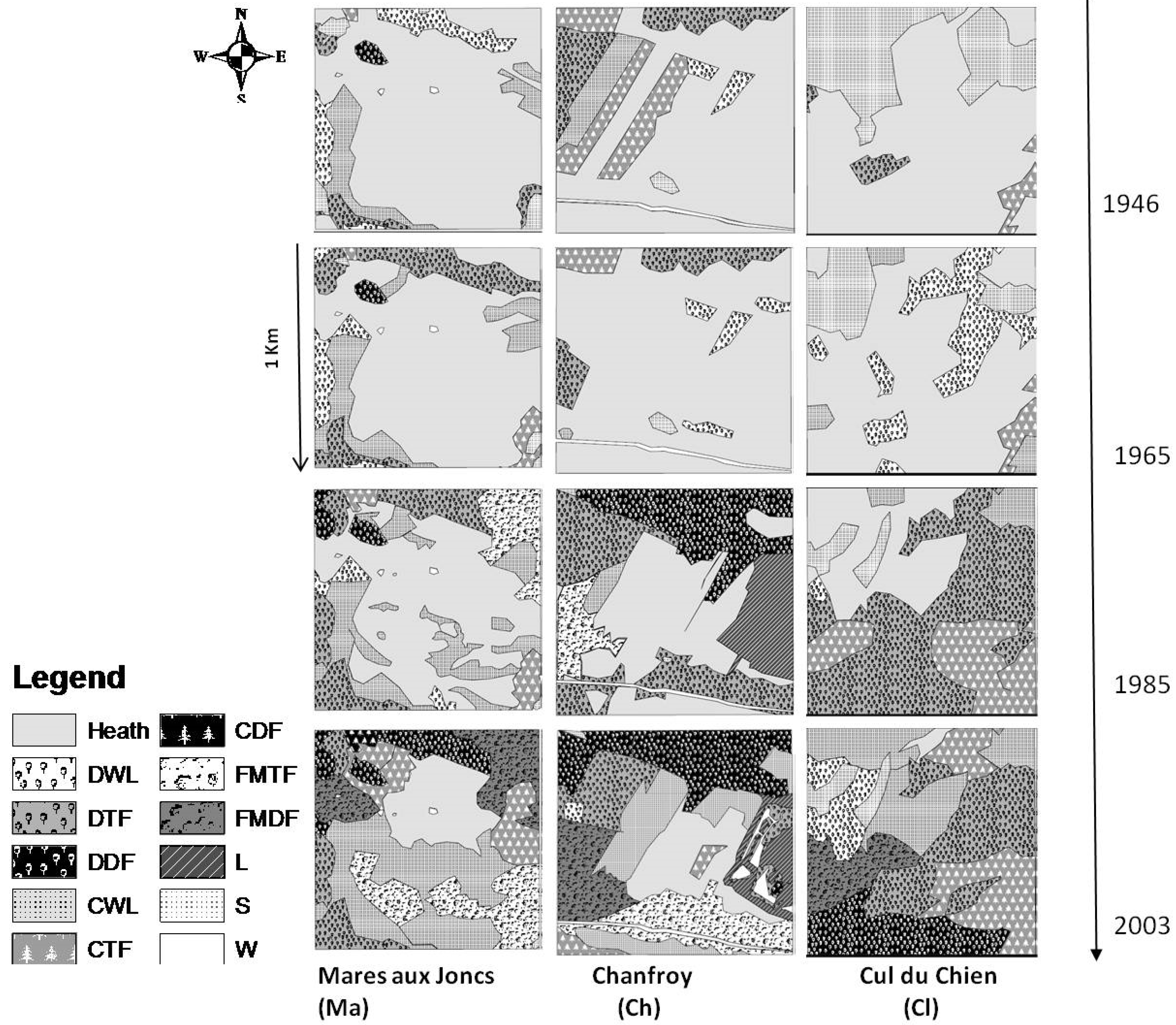
2.2.1. Classification of Changes in Vegetation Cover

The natural colonisation of the open areas was studied by photo interpretation of aerial photographs that were recorded during four aerial photographic surveys by the Institut Géographique National in the years 1946, 1965, 1985 (black and white orthorectified photos), and a 2003 digital colour picture with a spatial resolution 50 cm. The classification of vegetation cover was based on a visual interpretation method. Each image was overlain with a 50 m × 50 m grid and each cell was then classified into one of six classes of vegetation: Bare soil, Heathland, Grasslands, Conifer forests, Deciduous forests, and Mixed forest. The “interpretational keys” employed here were: 1. Visible colour, 2. Height, 3. Texture, and 4. Shape of objects [22]. Aerial photographic surveys in 2003 from BD ORTHO® IGN 2003 consist of real colour pictures closely resembling what would be observed by human eyes, used here to distinguish between different vegetation types: the conifers are dark green to blue-green in colour, deciduous trees are light green to yellow-green in colour, patches of grasses are yellow-green, heathlands are greenish grey, and bare soil is almost white sand. Old aerial photographs from 1946–1985 are black-and-white pictures; their tone is based on shades of grey. We were still able to distinguish between bright objects such as deciduous trees and grasses and dark objects such as conifer trees and dwarf shrub heath. Areas of homogeneous colour in the image corresponding to different land cover types were discriminated due to the presence of shadows, which were indicative of forest-type elements (e.g., large individual trees, forest stands). Texture is an important factor in the visual interpretation process, used here in particular to distinguish between the smooth texture of homogeneous grassland and the coarse texture of heathland. The shape of the tree crowns was used as an indicator to distinguish the type of tree, i.e., deciduous or conifer. Conifers are conical in shape while deciduous trees have billowy or tufted crowns.
The discrimination of forests was dependent on the dominant species in each pixel, with a threshold of 75% of the pixel covered. When conifer or deciduous species were above this threshold, the cell was classified as Coniferous or Deciduous forests, respectively. If neither of these groups reached the threshold, the cell was classified as Mixed forests. This classification was refined using the forest cover classification (IFN IF 2006, Table 1) [23].
Table 1. List of the different vegetation categories used during the photo interpretation process.
ClassesRanking CriteriaLand CoverAbbreviations
Absence of vegetationBare Soil (sand)S
Low stratumAbsence of trees and the presence of low-lying shrubsHeathlandHeath
Low and homogeneous stratumAbsence of treesLawnL
Low and homogeneous stratum, presence of woody plantsCover of forest trees is lower than 10%; Conifers species represent over 75% of the total tree coverConifer WoodlandCWL
Low and homogeneous stratum, presence of woody plantsCover of forest trees is lower than 10%; Deciduous species represent over 75% of the total tree coverDeciduous WoodlandDWL
High stratum is dominant, canopy is openCover of forest trees is greater than or equal to 10% and lower than 40%; Conifers species represent over 75% of the total tree coverThin Conifer Forest CTF
High stratum is dominant, canopy is opencover of forest trees is greater than or equal to 10% and lower than 40%; Deciduous species represent over 75% of the total tree coverThin Deciduous ForestDTF
High stratum is dominant, canopy is openCover of forest trees is greater than or equal to 10% and lower than 40%; any group of trees reaches 75% of the total rate of canopy coverThin Mixed Forest (Conifer and Deciduous)FMTF
High stratum is dominant, canopy is closed and homogeneousCover of forest trees is greater than or equal to 40%; Conifers species represent over 75% of the total tree coverDense Conifer ForestCFD
High stratum is dominant, canopy is closed and homogeneousCover of forest trees is greater than or equal to 40%; Deciduous species represent over 75% of the total tree coverDense Deciduous ForestDFD
High stratum is dominant, canopy is closed and homogeneousCover of forest trees is greater than or equal to 40%; any group of trees reaches 75% of the total rate of canopy coverDense Mixed Forest (Conifer and Deciduous)FMDF
WaterWater bodiesW
To assess the accuracy of the classified maps, the classification results must be compared with reference data collected on the ground [24]. In our study area, “ground data” for old historical photographs are not available. Thus, we assess the accuracy of the classification maps only for the vegetation cover in 2003 by comparing the classification maps with data collected on the ground at 75 points where we surveyed the vegetation in 2008 (see Section 2.5 for more details).We consider here that changes between these five years are negligible for forest species that have a slow growth and a long lifetime. Changes for heathland fragmented patches in this period are negligible. Moreover the ONF has attempted to preserve them since the early nineties.
By grouping together all forest categories, we obtained the spatial patterns of secondary succession in three time frames: 1946–1965, 1965–1985, and 1985–2003. The non-forested zones, which were maintained in the majority of cases by the actions of the conservation managers, were considered as stable zones in terms of their vegetation dynamics.

2.2.2. Transition Matrices

Transition matrices were obtained by cross-tabulating the consecutive maps, providing transition matrices for the comparable temporal periods, respectively 19, 20, and 18 years. These matrices show the dynamic between different vegetation types during the study period. This takes temporal changes into account as well as spatial dimensions. The cross-tabulations were done using IDRISI [25].

2.3. Spatial Environmental Variables

2.3.1. Physiographic Variables

We computed secondary physiographic attributes-slope and aspect—using ArcGIS [26] with a digital elevation model at a spatial resolution of 2.5 m, developed in the context of this study as the input layer.

2.3.2. Soil Survey

Two approaches were applied to study soil properties:
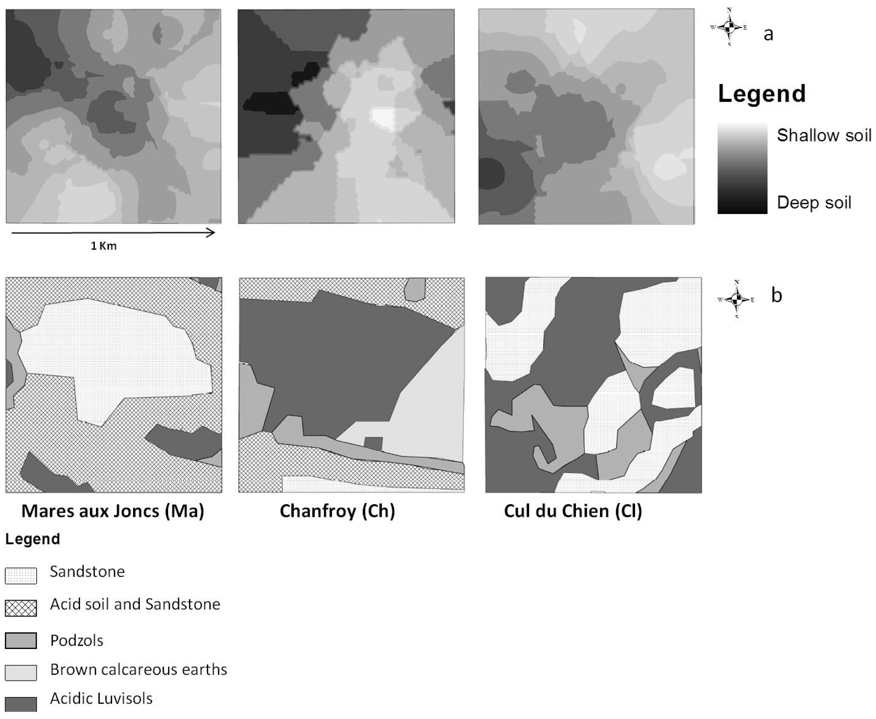
  • Soil depth data, acquired by field sampling. Measurements of soil depth were undertaken at 75 points, 25 points per site. A geostatistical study was conducted in order to obtain a raster map of soil depth based on the observation points [21]. To do this, we interpolated values at unobserved points using a kriging procedure. This method allows for the prediction of unknown values from data observed at known locations. Kriging uses variograms to express spatial variation and minimizes prediction errors by estimating the spatial distribution of predicted values [27,28]. Due to edge effects, the estimated values of soil depth at the plot edges might be subject to higher levels of uncertainty than other points within the plot boundaries. Three classes of soil depth were distinguished, in approximated accordance with observed soil horizons in this region [21]: shallow soils (0–20 cm), medium-depth soils (21–40 cm), and deep soils (greater than 40 cm). We used this interpolated map as a soil depth map as shown in Figure 2a.
  • Soil type data. To identify the distribution of soil types, we used a soil map of the region [29] at a spatial resolution of 2.5 m. Five soil types are found in the study area: brown calcareous earths, sandstone, acid soil and sandstone, podzols, and acidic luvisols, as shown in (Figure 2b).
Figure 2. Soil map: (a) soil depth, (b) soil type.
Ijgi 04 00957 g002

2.4. Spatial Data Analysis

To detect the influence of spatial environmental variables on the spatial expansion of secondary succession, two statistical approaches were used. First, a cross tabulation matrix indicating the number of pixels that coincide by category between combinations of two categorical raster maps was constructed. The Chi-square test was then applied to assess the significance of association between maps of secondary succession and the four spatial environmental variables, i.e., soil depth, soil type, slope, and aspect.
Subsequently, with the aim of identifying the similarities in location between the spatial patterns of secondary succession and each of the spatial environmental variables, we calculated the Kappa Location index (Kloc), which is an index that captures the spatial distribution of categories on a map, proposed by Pontius [30]. For the Kappa statistic (k), [31] provide guidelines for interpreting k values as follows: poor (k < 0), slight (0 < k < 0.20), fair (0.21 < k < 0.40), moderate (0.41 < k < 0.60), substantial (0.61< k< 0.80), and almost perfect (0.81 < k < 1.00). Kloc was calculated here using the Map Comparison Kit (MCK) software from the Research Institute for Knowledge Systems [32,33].
The categorical maps of the three time steps of forest expansion were compared on a pixel-by-pixel basis with soil and topography parameters, Kloc was calculated for each case.

2.5. Description of Current Forest Structure

In addition to spatiotemporal changes based on the transition matrices, we identified tree species composition and forest structure in different stands according to the forest’s age for the year 2008. In each of our study sites, a grid of 25 regularly spaced points every 200 m was randomly superimposed on the map. At each point we surveyed the vegetation according to the methodology developed by Braun-Blanquet [34] and measured the height of woody individuals on a surface which varied according to the tree density, i.e., 64 m2 for woodlands, where the cover of forest trees is less than 10%, and 200 m2 for forested areas, where the cover of forest trees is greater than 10% [35].

3. Results

3.1. Classification Accuracy Assessment

The overall accuracy of the vegetation map in 2003 is 0.84, with 63 pixels classified in the same way by photo interpretation and ground survey. The errors include principally mixed forest, which were overestimated here. These can be explained by the difference in the analysed surface between field and aerial photographs.

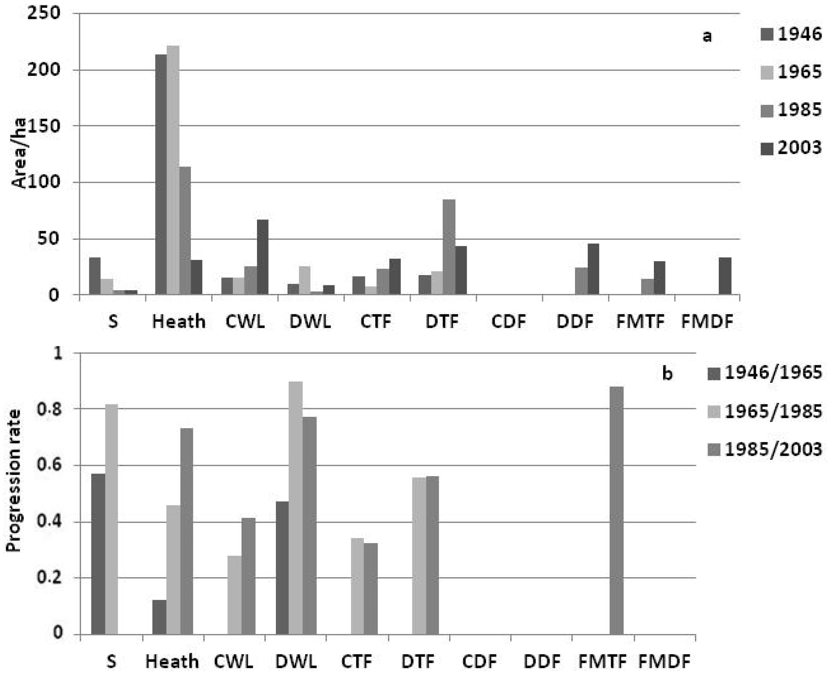
3.2. Landscape Dynamics

A comparison of surfaces with various vegetation categories over the years since 1946 showed a reduction in heathland areas over time with an increase in the progression rate over these periods (see Figure 3a,b). Over 60 years, more than 75% of the heathland has been progressively colonised by woody species (see Table 2). This change has generated a marked spatio-temporal heterogeneity in each of our three field sites as illustrated in Figure 4.
Figure 3. (a) Changes in area (ha) of the different dynamic stages between 1946 and 2003. (b) Changes in change rate for each vegetation category calculated from the transition matrices of 1946–1965, 1965–1985, and 1985–2003 (e.g., the Heathland change rate is 0.13 between 1946 and 1965 and 0.73 between 1985 and 2003). Bare soil (S), Heathland (Heath), Conifer woodland (CWL), Deciduous woodland (DWL), Conifer thin forest (CTF), Deciduous thin forest (DTF), Conifer dense forest (CDF), Deciduous dense forest (DDF), Mixed forest thin forest (FMTF), Mixed forest dense forest (FMDF).
Ijgi 04 00957 g003
Table 2. Transition matrices with the percentage of change from one stage to the other between the two dates: (a) 1946–1965, (b) 1965–1985, and (c) 1985–2003. The dark grey background represents the progressive transition of heathland to forest, a light grey background represents a regressive transition from forest to heathland related to anthropogenic activities, and underlined values indicate the no-change diagonal line of various physiognomic vegetation. The vegetation categories are explained in Table 1.
1965(a)1946
HeathCWLDWLCTFDTFCDFDDFFMTFFMDFSL
Heath0.880.370.610.450.32
CWL0.030.630.06
DWL0.070.530.16
CTF0.010.390.01
DTF0.020.470.540.03
CDF0.00
DDF1.00
FMTF0.00
FMDF0.00
S0.43
L0.00
1985(b)1965
HeathCWLDWLCTFDTFCDFDDFFMTFFMDFSL
Heath0.500.040.020.010.52
CWL0.070.68
DWL0.09
CTF0.080.180.640.03
DTF0.230.760.110.430.26
CDF0.00
DDF0.060.140.240.291.00
FMTF0.020.100.270.00
FMDF0.00
S0.18
L0.040.00
2003(c)1985
HeathCWLDWLCTFDTFCDFDDFFMTFFMDFSL
Heath0.27
CWL0.430.590.25
DWL0.070.23
CTF0.100.190.60
DTF0.070.44
CDF0.03
DDF0.150.060.271.00
FMTF0.130.230.080.120.12
FMDF0.370.150.070.88
S1.00
L1.00
Bare soil was mainly colonized by heathland species, i.e., 32% in the first time interval and 52% in the second, whereas colonisation of bare soil by woody species was less frequent, i.e., 16% and 26% in the first and second time intervals, respectively; this was principally due to colonization by deciduous forest communities (see Table 2a,b). During the two first periods studied, 1946–1965 and 1965–1985, heathland was colonised by deciduous communities DWL, DTF and DDF over 9% and 29% of the surface, respectively, while colonisation of heathland by conifers CWL, CTF was slower, accounting for 4% and 15%, respectively (see Table 2a,b). However, during the final period, 1985–2003, forest colonisation was faster and essentially due to conifers CWL, CTF, i.e., 53% as opposed to deciduous communities DWL at 7% and mixed forest species at 13% (Table 2c). Heathland colonised by deciduous communities (DWF) showed a fast phase of evolution between 1965 and 1985. Those heathlands tended to be colonised by thin deciduous species, which was different to other time-step comparisons; 76% of the area changed from DWF to DTF (Table 2b).
Figure 4. Habitat maps for 1946, 1965, 1985, and 2003. The grey scale palette used for presenting the maps aims at reflecting the secondary succession progression between open areas (clear colours) and woodlands (darker colours). Bare soil (S), Heathland (Heath), Conifer woodland (CWL), Deciduous woodland (DWL), Conifer thin forest (CTF), Deciduous thin forest (DTF), Conifer dense forest (CDF), Deciduous dense forest (DDF), Mixed forest thin forest (FMTF), Mixed forest dense forest (FMDF), Lawn (L), Water (W).
Ijgi 04 00957 g004
Woodlands reforested by conifers remained stable during the period 1946–1965. Twenty-eight percent of the surface area changed towards thin conifer forest and thin mixed forest during the period 1965–1985. This ratio increased to 42% over the period 1985–2003 (Figure 3b and Table 2). Thin conifer forests mainly changed to mixed or deciduous forests, most notably in the zones directly adjacent to deciduous forest areas (Figure 4). An important change in the forest cover over this period was also noted (Figure 5d). We observed an increase in dense deciduous forests and dense mixed forests at the expense of thin forest as illustrated in Figure 5b,c. However, the area of thin conifer forests increased, while the change in dense conifer forest was almost nil (see Figure 5a). Accordingly, we can clearly observe closure of open spaces, with an acceleration of this dynamic over time.
Figure 5. (a) Changes in area (ha) of conifers between 1946 and 2003: Conifer woodland (CWL), Conifer thin forest (CTF), Conifer dense forest (CDF). (b) Changes in area (ha) of deciduous between 1946 and 2003: Deciduous woodland (DWL), Deciduous thin forest (DTF), Deciduous dense forest (DDF). (c) Changes in area (ha) of mixed forest between 1946 and 2003: Mixed forest thin forest (FMTF), Mixed forest dense forest (FMDF). (d) Changes in area (ha) of different forest types: Deciduous (D), Conifer (C), Mixed forest (FM) between 1946 and 2003.
Ijgi 04 00957 g005

3.3. Influence of Spatial Environmental Variables on Forest Dynamics

The results showed that the dynamics of the forest were not independent of soil type (P < 0.0001), soil depth (P < 0.05), or the direction they faced (P < 0.05). However, there was no effect of slope on forest dynamics. Heathland without tree colonisation stands was spatially related to shallow soil (Kloc = 0.56), acid soil and sandstone (Kloc = 0.5), and flat topography (Kloc = 0.6). Recently colonised heathland stands, i.e., 1985–2003, were also related to acid soil and sandstone (Kloc = 0.4), medium-depth soils (Kloc = 0.4), and a south-facing aspect (Kloc = 0.39). Early recolonisations stands (1965–1985) showed a substantial degree of agreement with deep soil (Kloc = 0.52), acidic luvisols (Kloc = 0.43), and a north-facing aspect (Kloc = 0.6). The colonisation of tree species between 1946 and 1965 occurred preferentially on medium-depth and acidic luvisols (Kloc = 0.42). No other spatial preference was detected for this stand.

3.4. Forest Structure and Species Composition

Occupation by pine (Pinus sylvestris L.) in pure stands is higher in recently reforested zones, i.e., in the most recent 20 year period, while mixed stands of Pinus sylvestris and of Betula pendula Roth. are dominant in zones reforested between 20 and 40 years ago. Oak-pine stands composed of Pinus sylvestris and Quercus robur L. dominate in zones that were reforested during the previous 40 years, while those zones which contain older forests are principally occupied by two communities: Q. robur, Castanea sativa Mill., P. sylvestris, Pinus pinaster Aiton., and Q. robur, B. pendula, and P. sylvestris. The height measurements of individual trees varied from 11 m–20 m for zones afforested from 1946–1965 (60 years ago), 9 m–17 m in zones afforested from 1965–1985 (40 years ago), and 7 m–14 m in zones afforested from 1985–2003 (up to 20 years ago).

4. Discussion

The landscape changes observed during this period correspond to a drastic change in the use of the land by humans. Until the beginning of the 1960s this area of forest was privately owned, which explains the disappearance of the woody forest between 1946 and 1965 due to anthropogenic activities. Among historical activities in this region there are also the old quarries in Chanfroy, which explains the appearance of grasslands in this site during the period 1965–1985, which results from the rehabilitation of quarries.
Natural vegetation succession restarted after the cessation of traditional agro-pastoral activities and woodland exploitation. In the two first periods we studied, i.e., between 1946 and 1985, we detected the expansion of heathland to the detriment of bare soil (Table 2a,b), while the colonisation of bare soils by woody species was lower over this period. Colonisation by Calluna vulgaris [36], a primary succession species [34], was favoured by local edaphic conditions: sandy, acidic soils making colonisation by other woody species difficult.
We observed an acceleration in colonisation by woody species over time. Heathland that had been removed from human influence for the longest period had the greatest probability of being colonised by woody species. Two explanations can be proposed for this increase over time. First, the ageing of the heathland corresponding to the end of the life cycle of C. vulgaris, which is estimated to be about 35 years [37]. At this time the heathland entered into a phase of degeneration, corresponding to invasion by woody species on a more hospitable soil. Competition with woody species prevented the start of the Calluna life cycle [38] and therefore favoured colonisation by woody species in the available free space. Secondly, at the beginning of forest expansion, a front of colonisation started around the existing forest zone (Figure 5) and this was associated with the closure of the existing woodland zones (Table 2). However, direct colonisation by woody species in the open zones was more frequent during the most recent period in the dynamic (see Figure 4), and this increased the speed of heathland afforestation. Such spatial dynamics correspond to the classical conception of recolonisation by woody species [39,40], suggesting that anemochorous and heliophilous woody pioneer species have two colonisation strategies: either by dispersal with direct colonisation into open environments, or by expansion in proximity to an established forest. In our study sites, P. sylvestris was one of the two main pioneer woody species. Debussche & Lepart [41] and Debain [42], working on this species, showed that its principal front of colonisation was situated a few tens of meters around old pine stands, and individuals that have become established ahead of the colonisation front of old pine stands colonise the space around them. Here, the maturity of the woody populations that were present prior to 1946 permitted the colonisation of heathland relatively quickly. The colonisation that spreads from ahead of the front by the dispersed individuals or isolated individuals is slowed by the time necessary for the individuals to reach reproductive age. That means it is 15 years or more for P. sylvestris [43] and 20 years for B. pendula [44] before these dispersed individuals can begin colonising their surroundings, leading to the progressive closure of vegetation cover.
Understanding the differential colonisations of abandoned heathland by deciduous and conifer species allows the complex process of natural succession and its dynamics to be analysed. The dynamics of deciduous species during the period 1965–1985 come partly from closure of open woodland zones by deciduous pioneer species, and partly from the colonisation of open spaces (see Figure 4b and Table 2b). For the period 1985–2003, the dynamics of deciduous species were essentially limited to the closure of existing woody zones. We noticed that colonisation of woody species during this period is essentially by conifer species, with a significant increase in the surface occupied by pines. This conifer expansion has also been observed in another site in this region [11].
Several explanations can be proposed to explain the colonisation by conifers over the period 1985–2003. First, the spatial continuity of this colonisation can be explained by the capacity of the conifer to colonise and grow on shallow and poor soils where deciduous pioneer species are unable to establish a foothold (Figure 5a). P. sylvestris is able to colonise poor, dry soils [43,45]. The afforestation over this period could therefore be linked to the colonisation of conifer species in zones unfavourable to deciduous species, the most favourable areas being already colonized by deciduous species. This hypothesis has been confirmed through the results of the soil survey. We noticed two phases of woody species colonisation during this period according to the suitability of the soil conditions: fertile luvisols and deep soil. The first phase is marked by the colonisation of favourable zones by deciduous species and the closure of forest vegetation cover, progressively forming a mature forest. During the second phase, conifer species colonise those zones where soil conditions are unsuited to the installation of deciduous species, i.e., poor and shallow soils such as acid soil and sandstone.
Secondly, the rapid climate warming recorded in the French metropolitan area from the 1980s onwards [46,47], and the seasonal precipitation changes, especially a lowering of summer rainfall [47,48], has resulted in a period of drought that may have constituted a selective advantage for P. sylvestris due to its low water requirements and optimal stomatal regulation [49]. Thirdly, these climatic variations may have had consequences for the phenology and duration of the season of vegetation. Menzel and Fabian [50] have shown a lengthening of the active growth season since the 1960s. This phenomenon could be favourable to conifers by increasing their annual photosynthetic production due to their being able to use the solar radiation available in winter and early spring.
Among the factors studied here, soil types and soil depth greatly determine the direction of the dynamics of the forest. Concerning the influence of physiographic variables on the dynamics of the forest, the orientation of the slopes has an effect on the dynamics of vegetation such that we observed the persistence of heathland on warmer south-facing slopes that are more suitable for dry heathland vegetation. Northern slopes are moister, and colonisation by trees and other shrubs is more obvious there. No effect of the steepness of the terrain (slope gradient) was detected, which can be explained by the fact that steep slopes are a marginal land for agriculture and had been abandoned before 1946, the year in which dynamic monitoring in our study began.
Using aerial photographs to create ecosystems maps is not an error free process; quantitative and/or qualitative errors are possible, caused by digitization, georeferencing, measurement, classification, and interpolation errors [51]. For this reason spatial uncertainties in our input historical data could not be estimated due to the absence of ground data, and error propagation related to input uncertainty has not been assessed.

5. Conclusion and Implications for Land Management

Our study documents the recolonisation of heathland by forests, with a loss of more than 75% of heathland areas during the last 60 years. Nevertheless, this colonisation varies temporally and spatially, as the process of forest recolonisation depends on several factors: the mechanisms underlying woody species dynamics, the ecological niches of the different species, and the spatial variability in soil and climatic conditions within the site.
The relevance of this study is to highlight the importance of taking the spatial and temporal factors into account for the conservation management of heathland; this concept has not been applied or proposed in any previous study of heathland management.
Our results show that the temporal factor is very important because heathland is not colonised at the same speed over time. Taking into account this information, coupled with preferable spatial factors for heathland persistence, could be a great benefit for heathland management. It also has the potential to assist land managers in selecting those heathland areas that will be easier to conserve and/or to restore, by focusing on areas and spatial conditions that prevent reforestation and hence favour long-term stability of the heathland. According to our results, management priority should be given to those heathlands that are located on shallow soils, on level planes, or south-facing sites, and far from the borders of mature forests.

Acknowledgments

We thank the ONF, in particular the Unit of Ecological Support, for providing the necessary data for this study.

Author Contributions

Samira Mobaied designed and coordinated the study, performed the field work, processed spatial data analyses and prepared and drafted the manuscript; the article was improved by the substantial contributions of Nathalie Machon at various stages of the analysis and writing process. Arnauld Lalanne contributed substantially to data acquisition and interpretation of results. Bernard Riera made substantial contributions to conception and design of the study, fieldwork, methods and data acquisition. All authors read and approved the final manuscript.

Conflicts of Interest

The authors declare no conflict of interest.

References

  1. Foley, J.A.; Defries, R.; Asner, G.P.; Barford, C.; Bonan, G.; Carpenter, S.R.; Chapin, F.S.; Coe, M.T.; Daily, G.C.; Gibbs, H.K.; et al. Global consequences of land use. Science 2005, 309, 570–574. [Google Scholar] [CrossRef] [PubMed]
  2. Rockstrom, J.; Steffen, W.; Noone, K.; Persson, Å.; Chapin, F.S., III; Lambin, E.F.; Lenton, T.M.; Scheffer, M.; Folke, C.; Schellnhuber, H.J.; et al. A safe operating space for humanity. Nature 2009, 24, 472–475. [Google Scholar]
  3. EC Habitats Directive. Council Directive 92/43/EEC of 21 May 1992 on the Conservation of Natural Habitats and of Wild Fauna and Flora; European Commission: Brussels, Belgium, 1992. [Google Scholar]
  4. Ausden, M. Habitat Management for Conservation; A Handbook of Techniques; Oxford University Press: Oxford, UK, 2007; p. 384. [Google Scholar]
  5. Thompson, D.B.A.; MacDonald, A.J.; Marsden, J.H.; Galbraith, C.A. Upland heather moorland in Great Britain: A review of international importance, vegetation change and some objectives for nature conservation. Biol. Conserv. 1995, 71, 163–178. [Google Scholar] [CrossRef]
  6. Usher, M.B. Management and diversity of arthropods in Calluna heathland. Biodivers. Conserv. 1992, 1, 63–79. [Google Scholar] [CrossRef]
  7. Usher, M.B.; Thompson, D.B.A. Variation in the upland heathland of Great Britain: Conservation importance. Biol. Conserv. 1993, 66, 69–81. [Google Scholar] [CrossRef]
  8. Webb, N.R. The traditional management of European heathlands. J. Appl. Ecol. 1998, 35, 987–990. [Google Scholar] [CrossRef]
  9. Webb, N.R. Atlantic heathland. In Davy Handbook of Ecological Restoration; Martin, R.P., Anthony, J., Eds.; Cambridge University Press: Cambridge, UK, 2008; Volumes 1 and 2, pp. 401–418. [Google Scholar]
  10. Price, E.A.C. Lowland Grassland and Heathland Habitats; Routledge: London, UK, 2003. [Google Scholar]
  11. Mobaied, S.; Riera, B.; Lalanne, A.; Baguette, M.; Machon, N. The use of diachronic spatial approaches and predictive modelling to study the vegetation dynamics of a managed heathland. Biodivers. Conserv. 2011, 20, 73–88. [Google Scholar] [CrossRef]
  12. Barker, C.G.; Power, S.A.; Bell, J.N.B.; Orme, C.D.L. Effects of habitat management on heathland response to atmospheric nitrogen deposition. Biol. Conserv. 2004, 120, 41–52. [Google Scholar] [CrossRef]
  13. Wamelink, G.W.W.; de Jong, J.J.; van Dobben, H.F.; van Wijk, M.N. Additional costs of nature management caused by deposition. Ecol. Econ. 2005, 52, 437–451. [Google Scholar] [CrossRef]
  14. Calvo, L.; Alonso, I.; Marcos, E.; de Luis, E. Effects of cutting and nitrogen deposition on biodiversity in Cantabrian heathlands. Appl. Veg. Sci. 2007, 10, 43–52. [Google Scholar] [CrossRef]
  15. Fagundez, J. Heathlands confronting global change: Drivers of biodiversity loss from past to future scenarios. Ann. Bot. 2013, 111, 151–172. [Google Scholar] [CrossRef] [PubMed]
  16. Miles, J. Vegetation Dynamics; Chapman and Hall: London, UK, 1979. [Google Scholar]
  17. Evans, F.C.; Dhal, E. The vegetational structure of an abandoned field in southeastern Michigan and its relations to environmental factors. Ecology 1955, 36, 685–706. [Google Scholar] [CrossRef]
  18. Dargie, T.C.D. An ordination analysis of vegetation patterns on topoclimate gradients in South-East Spain. J. Biogeogr. 1987, 14, 197–211. [Google Scholar] [CrossRef]
  19. Badano, E.I.; Cavieres, L.A.; Molina-Montenegro, M.A.; Quiroz, C.L. Slope aspect influences plant association patterns in the Mediterranean matorral of central Chile. J. Arid Environ. 2005, 62, 93–108. [Google Scholar] [CrossRef]
  20. Tilman, D.; Kareiva, P. Spatial Ecology: The Role of Space in Population Dynamics and Interspecific Interactions; Princeton University: Princeton, NJ, USA, 1997; p. 368. [Google Scholar]
  21. Mobaied, S.; Ponge, J.F.; Salmon, S.; Lalanne, A.; Riera, B. Influence of the spatial variability of soil type and tree colonization on the dynamics of Molinia caerulea (L.) Moench in managed heathland. Ecol. Complex. 2012, 11, 118–125. [Google Scholar] [CrossRef]
  22. James, S.A.; Irene, M.; Johannes, R. Small-Format Aerial Photography: Principles, Techniques and Geoscience Applications; Elsevier Science: Trier, Germany, 2010; p. 268. [Google Scholar]
  23. Derrière, N.; Lucas, S. La Forêt Française en 2005 Résultats de la Première Campagne Nationale Annuelle; IFN: Saint-Mandé, France, 2006; p. 8. [Google Scholar]
  24. Ross, S.L.; John, G.L. Remote Sensing and GIS Accuracy Assessment; U.S. Environmental Protection Agency (EPA): Washington, DC, USA, 2011; p. 320.
  25. IDRISI, version Andes 32; Clark University: Worcester, OH, USA, 1987–2006.
  26. ESRI ArcGIS, version 9.2; Environmental Systems Research Institute Inc.: Redlands, CA, USA, 2006.
  27. Isaaks, E.H.; Srivastava, R.M. An Introduction to Applied Geostatistics; Oxford University Press: New York, NY, USA, 1989; p. 561. [Google Scholar]
  28. Krige, D. A statical problem to some basic minim valuation problems on the Witwatersrand. J. Chem. Metall. Min. Soc. S. Afr. 1951, 52, 119–139. [Google Scholar]
  29. Institut Géographique National (France). Soil Map of Forêt de Trois Pignons ONF/ED EDR25©IGN2006 [map]; Technical report for Forêt Domaniale des Trois Pignons; Office National des Forêts: Paris, France, 2006.
  30. Pontius, R.G. Quantification error versus location error in comparison of categorical maps. Photogramm. Eng. Remote Sens. 2000, 66, 1011–1016. [Google Scholar]
  31. Landis, J.R.; Koch, G.G. The measurement of observer agreement for categorical data. Biometrics 1977, 33, 159–174. [Google Scholar] [CrossRef] [PubMed]
  32. Visser, H.; de Nijs, T. The map comparison kit MCK software. Environ. Modell. Softw. 2006, 21, 346–358. [Google Scholar] [CrossRef]
  33. Map Comparison Kit 3. Available online: www.riks.nl (accessed on 21 February 2014).
  34. Braun-Blanquet, J. Plant Sociology; McGraw-Hill Book Company: New York, NY, USA, 1932; p. 438. [Google Scholar]
  35. Milan, C.; Zdenka, O. Plot sizes used for phytosociological sampling of European vegetation. J. Veg. Sci. 2003, 14, 563–570. [Google Scholar]
  36. Gimingham, C.H. Ecology of Heathland; Chapman and Hall: London, UK, 1972; p. 266. [Google Scholar]
  37. Walker, L.R.; Walker, J.; Hobbs, R.J. Linking Restoration and Ecological Succession; Springer: New York, NY, USA, 2007. [Google Scholar]
  38. Gimingham, C.H. A reappraisal of the cyclical processes in Calluna heathland. Vegetation 1988, 77, 61–64. [Google Scholar] [CrossRef]
  39. Grime, J.P.; Hodgson, J.G.; Hunt, R. Comparative Plant Ecology: A Functional Approach to Common British Species; Unwin Hyman: London, UK, 1988; p. 742. [Google Scholar]
  40. Rameau, J.C.; Mansion, D.; Dumé, G. Flore Forestière Française; Institut pour le Développement Forestier: Dijon, France, 1993; p. 2421. [Google Scholar]
  41. Debussche, M.; Lepart, J. Establishment of woody plants in Mediterranean old fields: Opportunity in space and time. Landsc. Ecol. 1992, 6, 133–145. [Google Scholar] [CrossRef]
  42. Debain, S.; Curt, T.; Lepart, J.; Prevosto, B. Reproductive variability in Pinus sylvestris in southern France: Implications for invasion. J. Veg. Sci. 2003, 4, 509–516. [Google Scholar] [CrossRef]
  43. Richardson, D.M. Ecology and Biogeography of Pinus; Cambridge University Press: Cambridge, UK, 1988; p. 546. [Google Scholar]
  44. Scherer-Lorenzen, M.; Körner, C.; Schulze, E.D. Temperate and boreal systems. In Forest Diversity and Function; Springer: Berlin, Germany, 2005; pp. 377–390. [Google Scholar]
  45. Cañellas, I.; Martínez García, F.; Montero, G. Silviculture and dynamics of Pinus sylvestris L. stands in Spain. Investig. Agrar. Sist. Recur. For. 2000, 1, 233–253. [Google Scholar]
  46. Bessemoulin, P.; Mestre, O. Le réchauffement climatique sur le siècle en France. Fr. Chang. Glob. 2001, 12, 32–34. [Google Scholar]
  47. Canellas, C.; Gibelin, A.L.; Lassègues, P.; Kerdoncuff, M.; Dandin, P.; Simon, P. Les normales climatiques spatialisées Aurelhy 1981–2010: Températures et précipitations. La Météorol. 2014, 85. [Google Scholar] [CrossRef]
  48. Moisselin, J.M. Les précipitations en France au XXème siècle. Fr. Chang. Glob. 2002, 13, 57–62. [Google Scholar]
  49. Dulamsuren, C.; Hauck, M.; Bader, M.; Oyungerel, S.; Osokhjargal, D.; Nyambayar, S.; Leuschner, C. The different strategies of Pinus sylvestris and Larix sibirica to deal with summer drought in a northern Mongolian forest-steppe ecotone suggest a future superiority of pine in a warming climate. Can. J. For. Res. 2009, 39, 2520–2528. [Google Scholar] [CrossRef]
  50. Menzel, A.; Fabian, P. Growing season extended in Europe. Nature 1999, 397, 659–661. [Google Scholar] [CrossRef]
  51. Rocchini, D.; Foody, D.G.; Nagendra, H.; Ricotta, C.; Anand, M.; He, K.S.; Amici, V.; Kleinschmit, B.; Forster, M.; Schmidtlein, S.; et al. Uncertainty in ecosystem mapping by remote sensing. Comput. Geosci. 2013, 50, 128–135. [Google Scholar] [CrossRef]

