
Mapping the Socio-Economic and Ecological Resilience of Japanese Coral Reefscapes across a Decade

Abstract
:
1. Introduction
2. Methods
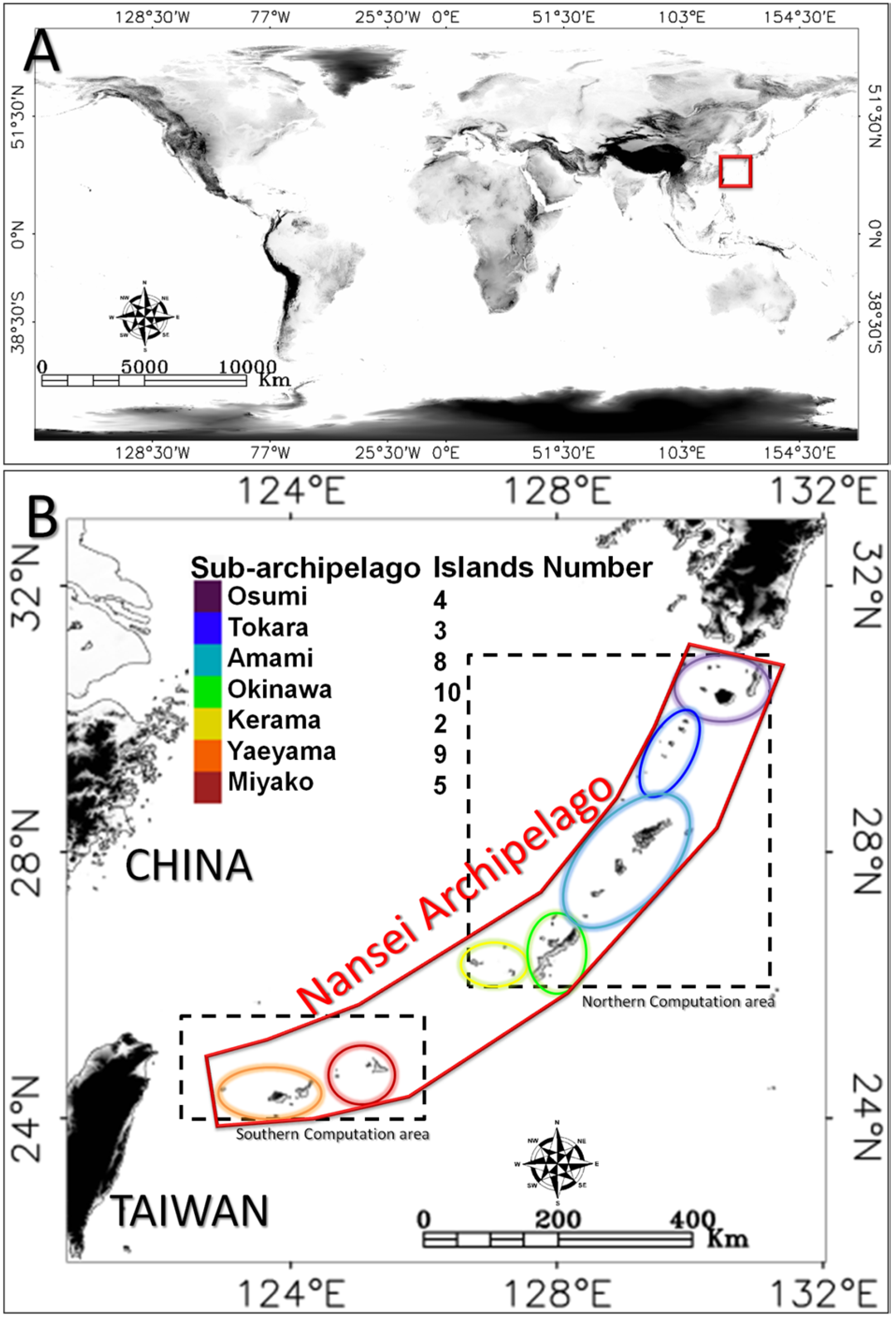
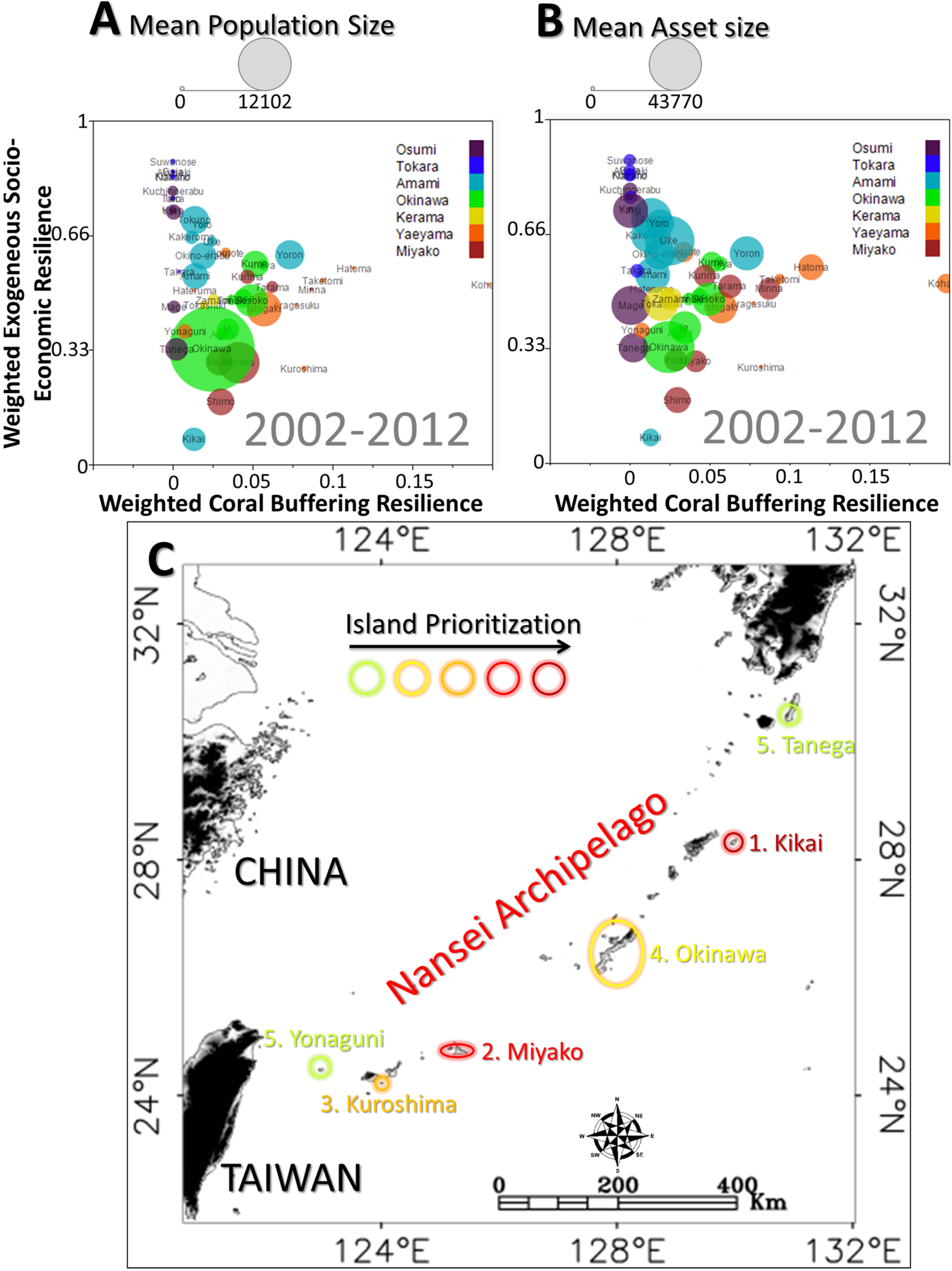
2.1. Study Region
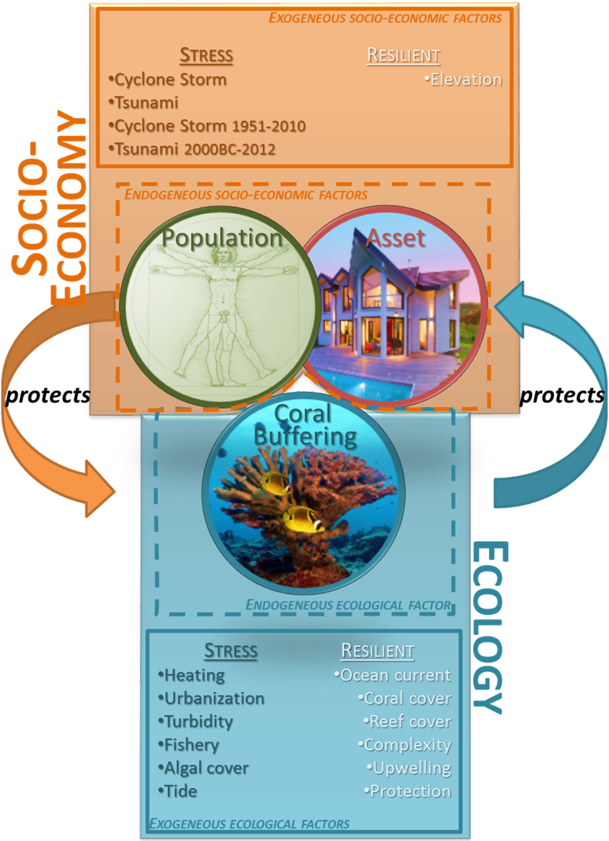
2.2. Linking the Socio-Economy and the Ecology

2.3. Socio-Economic Factors

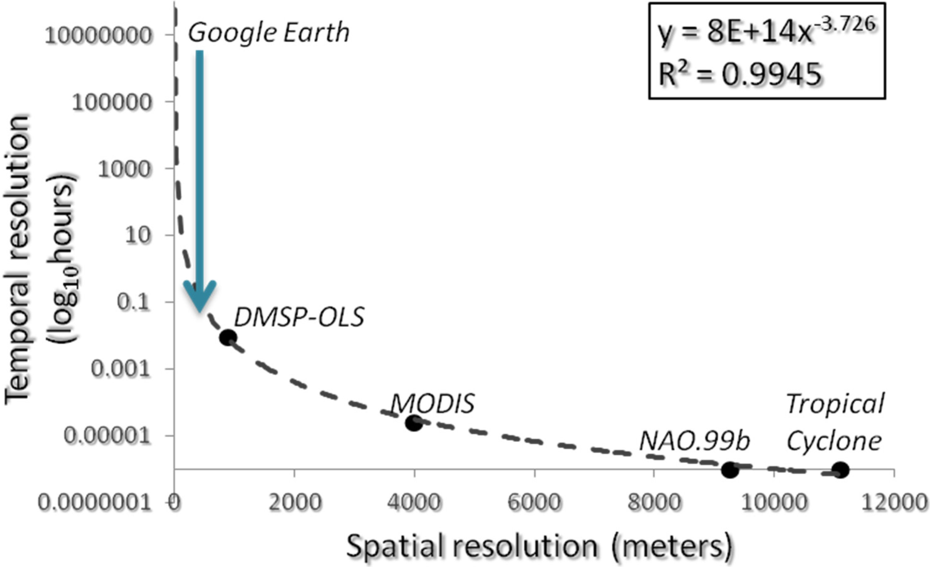
| Factor | Proxy | Source | Space Resolution | Time Resolution | Weight | Reference | |
|---|---|---|---|---|---|---|---|
| Stressor | Acute climatic hazards | Cyclone Storm | Tropical Cyclone Best-Track data | 1 arcsec | 2002–2012, 1 year | 2 | [33] |
| Acute oceanic hazards | Tsunami | Global Historical Tsunami Database | 1 arcsec | 2002–2012, 1 year | 2 | [34] | |
| Chronic climatic hazards | Cyclone storm (1951-2010) | Tropical Cyclone Best-Track data | 1 arcsec | 1951–2010 | 1 | [33] | |
| Chronic oceanic hazards | Tsunami (2000BC–2012AD) | Global Historical Tsunami Database | 1 arcsec | 2000BC–2012AD | 1 | [34] | |
| Resilient | Resistance to oceano-climatic hazards | Elevation | Global Digital Elevation Model (v.2) | 1 arcsec | 2011 | 3 | [24] |
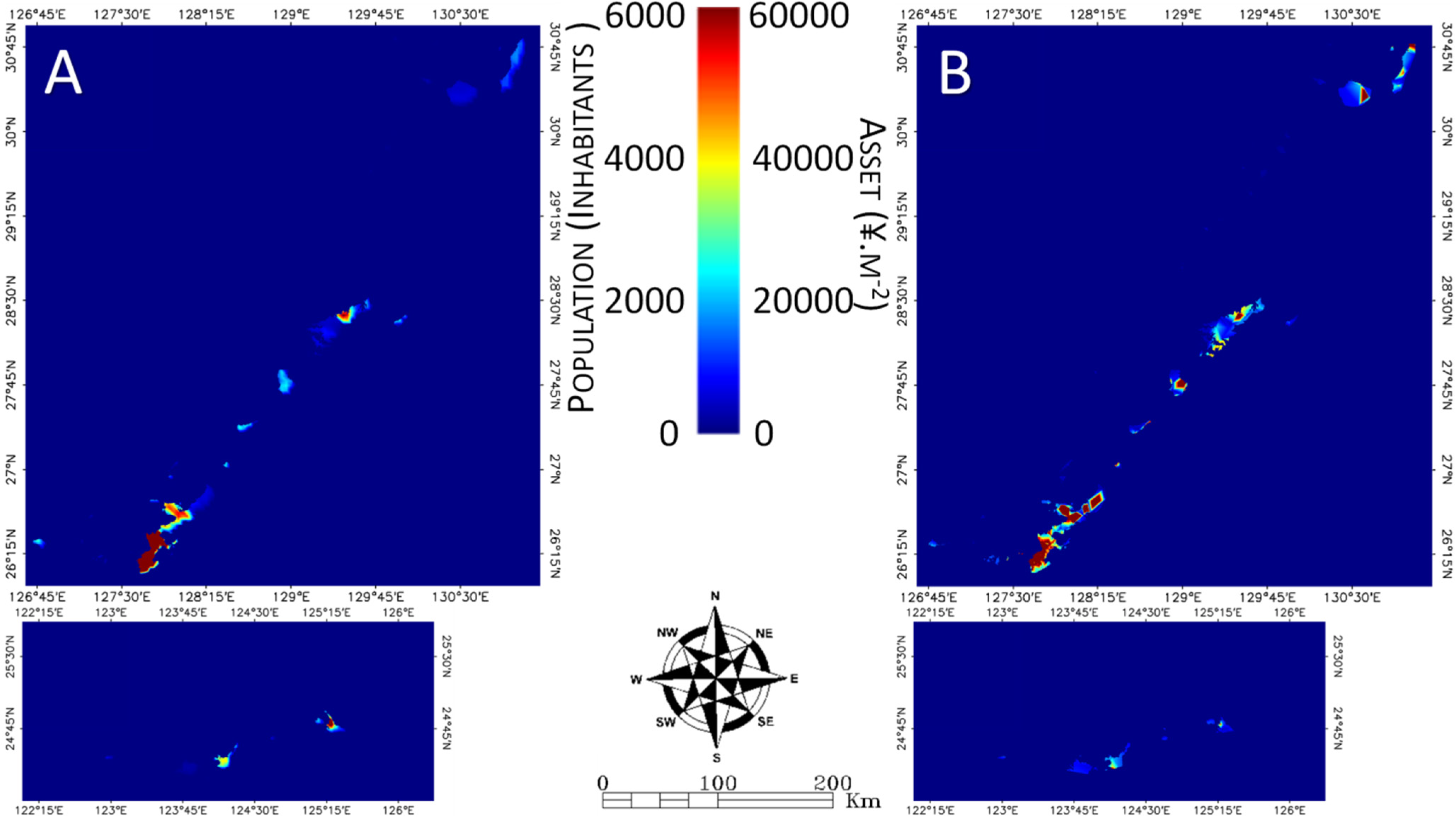
2.3.1. Population and Asset Endogenous Factors
2.3.2. Oceano-Climatic Stress Exogenous Factors
2.3.3. Elevation Resilient Exogeneous Factor
2.4. Ecological Factors
| Factor | Source | Space Resolution | Time Resolution | Weight | Reference | ||
|---|---|---|---|---|---|---|---|
| Stressor | Thermal stress | Heating rate | MODIS SST (11 μm) | 4 km | Summer 2002–2012, 1 week | 2 | [36,37,38] |
| Habitat-removal toxicity Algal competition | Urbanization | DMSP-OLS | 30 arcsec | 2002–2012, 1 year | 2 | [39,40] | |
| Sediment stress | Turbidity | MODIS Kd (490 nm) | 4 km | 2002–2012, 1 year | 1 | [41,42] | |
| Algal competition Anchor damage | Fishery | VHR Google Earth Professional | 2 m | 2013 | 1 | [3,43,44] | |
| Algal competition | Algal cover | ALOS/AVNIR-2- | 10 m | 2009–2010 | 1 | [45,46] | |
| Emersion adjustment | Tide exposure | NAO.99b tidal prediction system/Delft3D | 5 arcmin | Spring 2002–2012, 1 day | 1 | [47,48] | |
| Resilient | Connectivity | Ocean current | MODIS SST (11 μm) | 4 km | Winter 2002–2012, 1 week | 3 | [49,50] |
| Coral source | Coral cover | ALOS/AVNIR-2- | 10 m | 2009–2010 | 3 | [51] | |
| Habitat sink | Reef cover | ALOS/AVNIR-2- | 10 m | 2009–2010 | 2 | [52,53] | |
| Ecological niche | Bathymetric complexity | VHR Google Earth Professional | 2 m | 2013 | 2 | [54,55] | |
| Thermal cooling | Upwelling | GEBCO 08-grid | 30 arcsec | 2008 | 1 | [56] | |
| Removal of anthropogenic impacts | Protected Area | Protected Planet | 1 arcmin | 2013 | 1 | [57] |
2.4.1. Coral Buffering Endogenous Factor
| Habitat Class | Drag Coefficient (Cd) |
|---|---|
| Coral cover 50%–100% | 0.06 |
| Coral cover 5%–50% | 0.045 |
| Rock | 0.03 |
| Seaweed | 0.02 |
| Sand | 0.01 |
| Mud | 0.01 |
2.4.2. Stress Exogenous Factors
Thermal and Sediment Stress
Urbanization Stress
Fishery Stress
Algal Competitor Stress
Emersion Adjustment
2.4.3. Resilient Exogenous Factors
Connectivity
Coral Source and Habitat Sink
Ecological Niche
Thermal Cooling
Coral Protected Area
- 2002–2004, including 19 protected areas
- 2005–2006, including 20 protected areas (Kerama Shoto Coral Reef implementation)
- 2007–2011, including 21 protected areas (Ishigaki implementation)
- 2012, including 23 protected areas (Hateruma and Hatoma implementation)
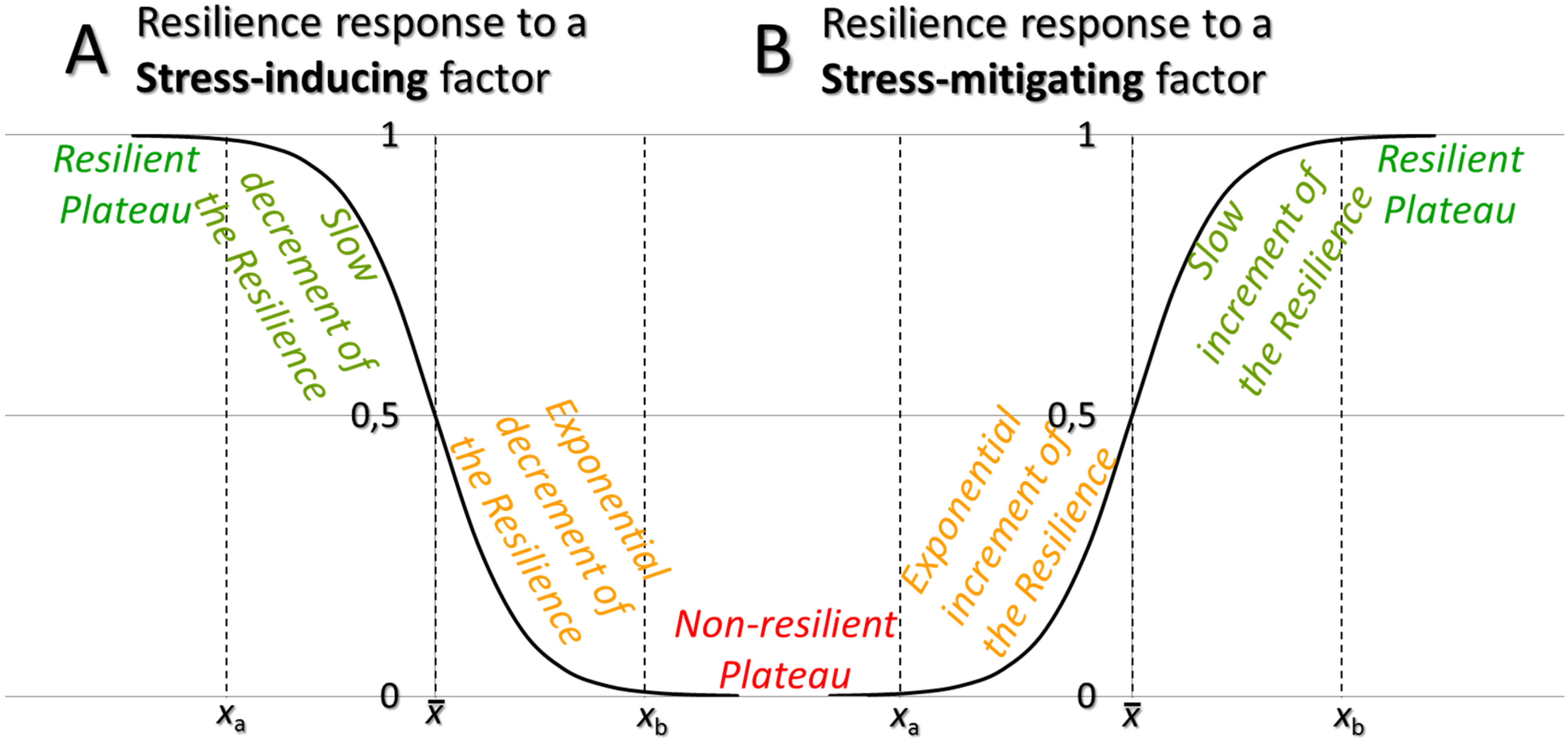
2.5. The Fuzzy Logic for the Socio-Economic and Ecological Resilience

3. Results
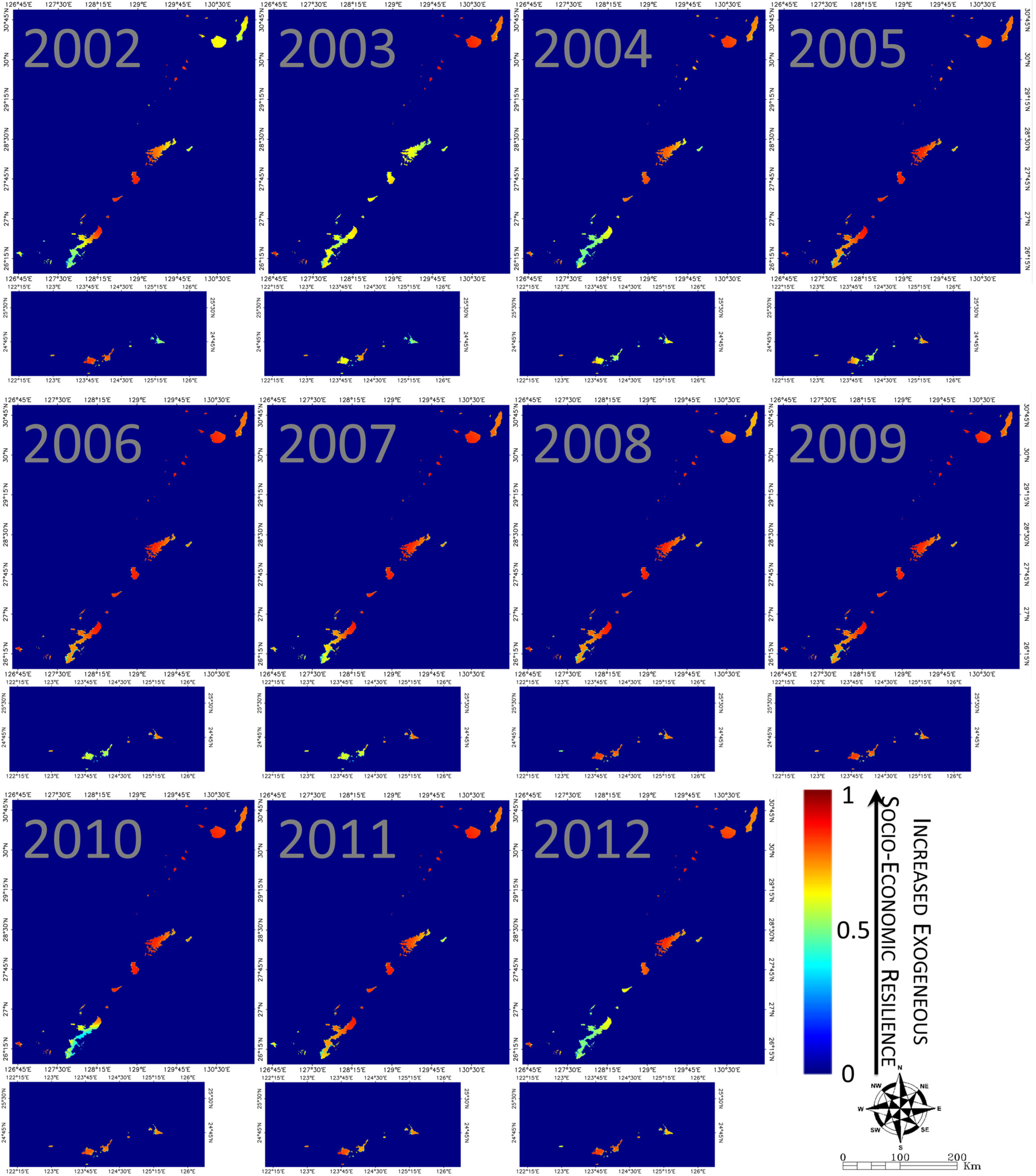
3.1. Socio-Economic and Ecological Regional Mapping


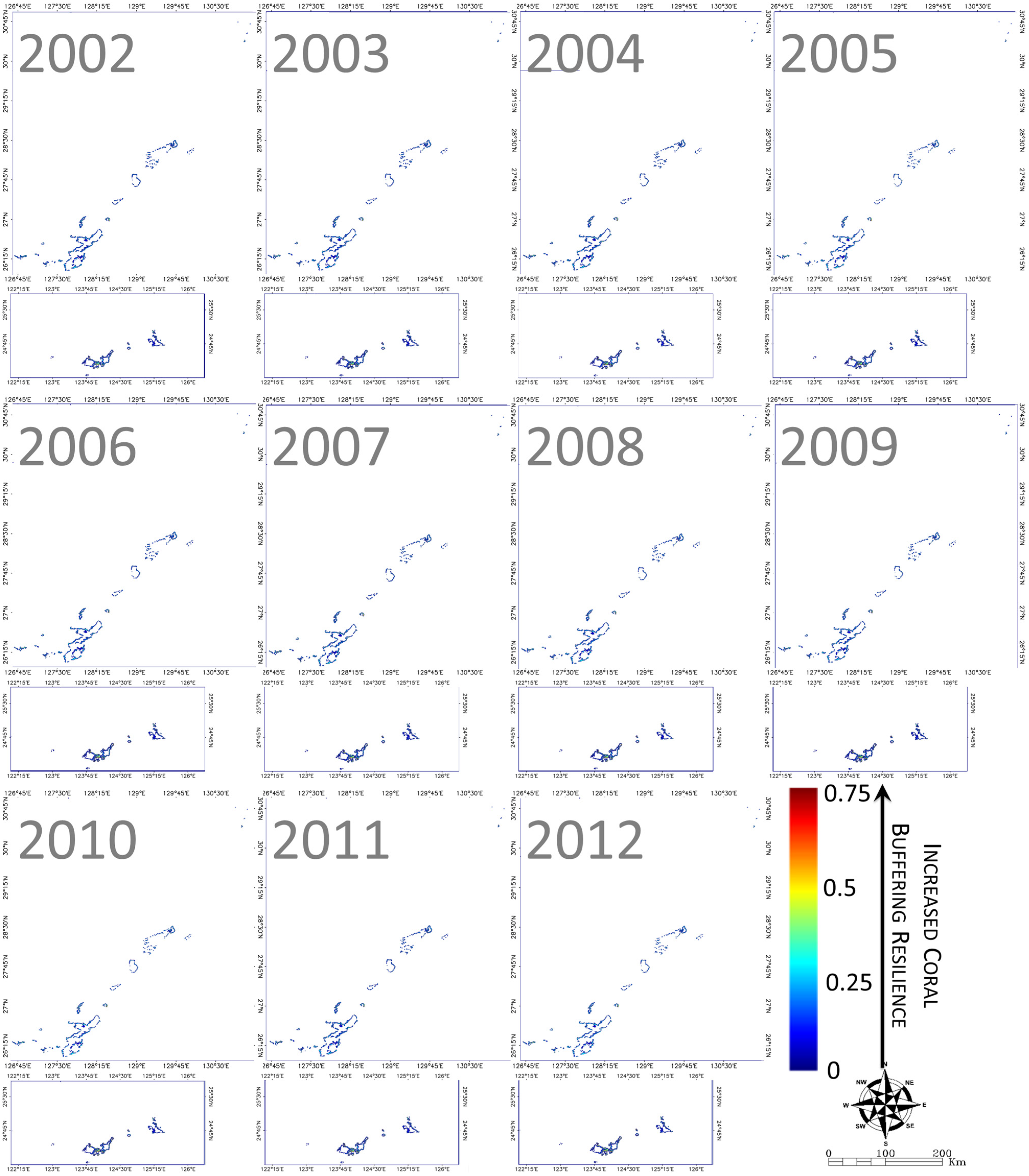
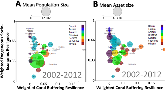
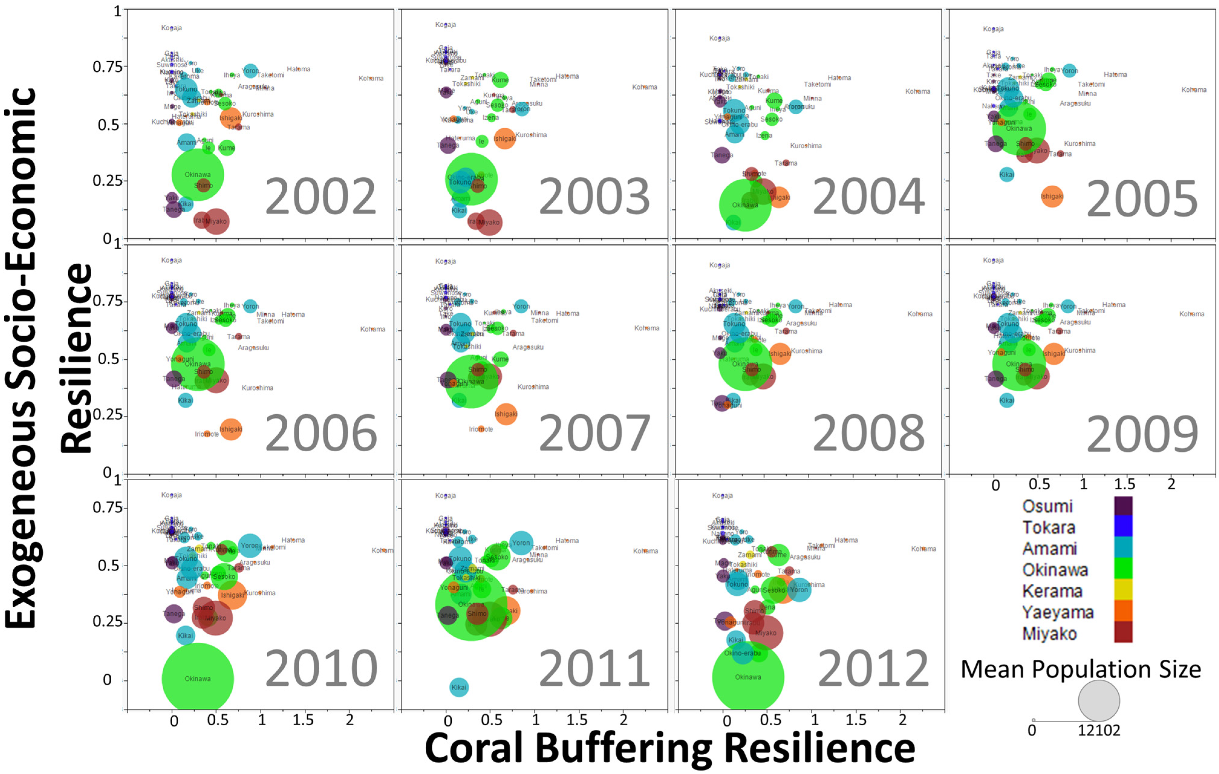
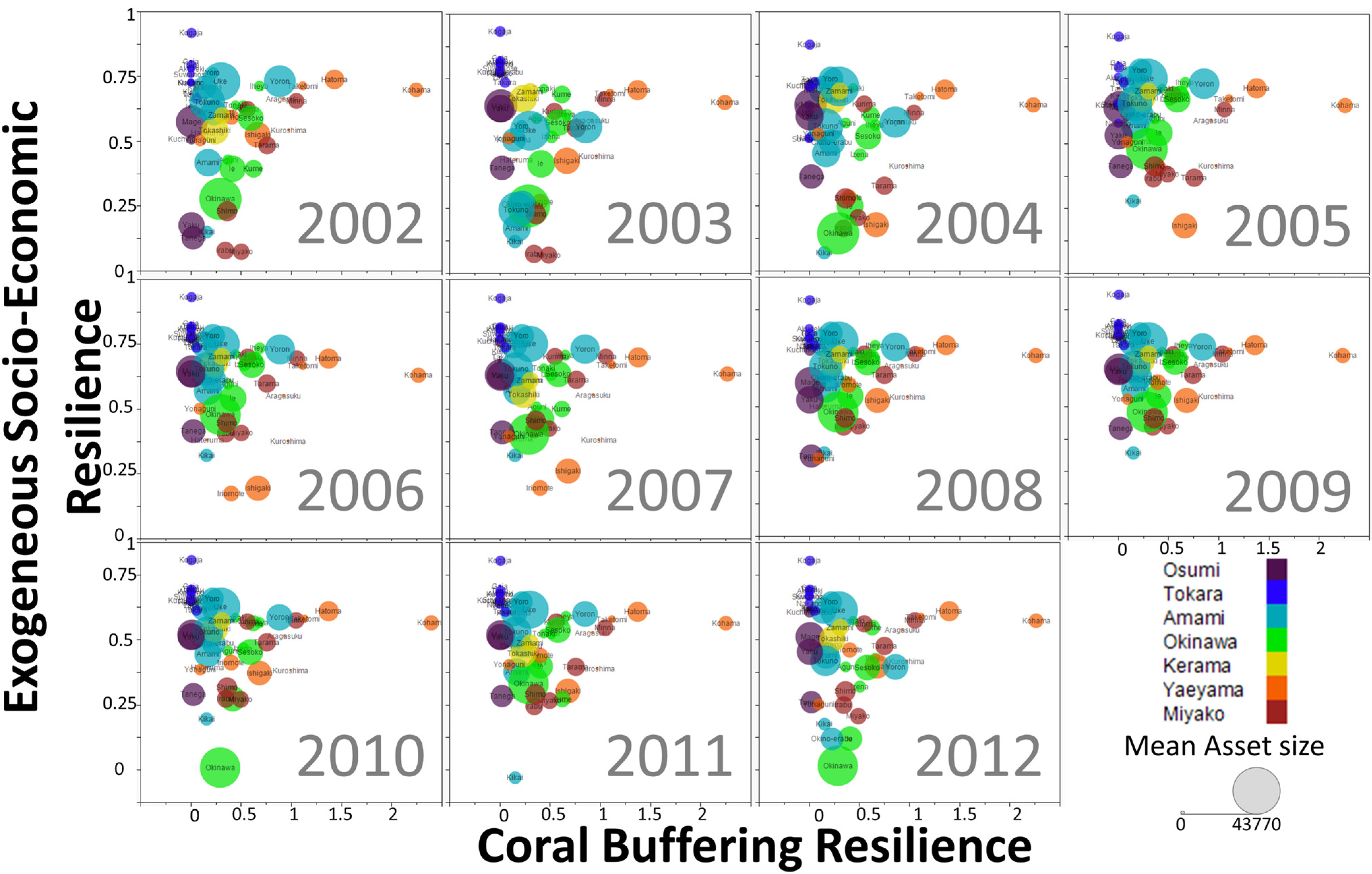
3.2. Local Socio-Economic and Ecological Patterns


4. Discussion
4.1. Factor Selection and Recommendations

4.2. Representing the Socio-Economic and Ecological Resilience

4.3. Guidance Implications

4.4. Limitations
5. Conclusions
Acknowledgments
Author Contributions
Conflicts of Interest
References
- Barbier, E.B.; Hacker, S.D.; Kennedy, C.; Koch, E.W.; Stier, A.C.; Silliman, B.R. The value of estuarine and coastal ecosystem services. Ecol. Monogr. 2011, 81, 169–193. [Google Scholar] [CrossRef]
- Costanza, R.; de Groot, R.; Sutton, P.; van der Ploeg, S.; Anderson, S.J.; Kubisszewski, I.; Farber, S.; Turner, R.K. Changes in the global value of ecosystem services. Global Environ. Chang. 2014, 26, 152–158. [Google Scholar] [CrossRef]
- Wilkinson, C. Status of Coral Reefs of the World: 2008; Global Coral Reef Monitoring Network and Reef and Rainforest Research Center: Townsville, QLD, Australia, 2008; p. 298. [Google Scholar]
- Bellwood, D.R.; Hughes, T.P.; Folke, C.; Nystrom, M. Confronting the coral reef crisis. Nature 2004, 429, 827–833. [Google Scholar] [CrossRef] [PubMed]
- Hoegh-Guldberg, O.; Mumby, P.J.; Hooten, A.J.; Steneck, R.S.; Greenfield, P.; Gomez, E.; Harvell, C.D.; Sale, P.F.; Edwards, A.J.; Caldeira, K.; et al. Coral reefs under rapid climate change and ocean acidification. Science 2007, 318, 1737–1742. [Google Scholar] [CrossRef] [PubMed]
- Nyström, M.; Folke, C. Spatial resilience of coral reefs. Ecosystems 2011, 4, 406–417. [Google Scholar]
- McClanahan, T.; Polunin, N.; Done, T. Ecological states and the resilience of coral reefs. Conserv. Ecol. 2002, 6, 18. [Google Scholar]
- Mumby, P.J.; Hastings, A.; Edwards, H.J. Thresholds and the resilience of Caribbean coral reefs. Nature 2007, 450, 98–101. [Google Scholar] [CrossRef] [PubMed]
- Roff, G.; Mumby, P.J. Global disparity in the resilience of coral reefs. Trends Ecol. Evol. 2012, 27, 404–413. [Google Scholar] [CrossRef] [PubMed]
- Nyström, M.; Graham, N.A.J.; Lokrantz, J.; Norström, A.V. Capturing the cornerstones of coral reef resilience: Linking theory to practice. Coral Reefs 2008, 27, 795–809. [Google Scholar] [CrossRef]
- Hughes, T.P.; Graham, N.A.; Jackson, J.B.; Mumby, P.J.; Steneck, R.S. Rising to the challenge of sustaining coral reef resilience. Trends Ecol. Evol. 2010, 25, 633–642. [Google Scholar] [CrossRef] [PubMed]
- Maynard, J.A.; Marshall, P.A.; Johnson, J.E.; Harman, S. Building resilience into practical conservation: Identifying local management responses to global climate change in the southern Great Barrier Reef. Coral Reefs 2010, 29, 381–391. [Google Scholar] [CrossRef]
- McClanahan, T.R.; Donner, S.D.; Maynard, J.A.; MacNeil, M.A.; Graham, N.A.J.; Maina, J.; Baker, A.C.; Alemu I., J.B.; Beger, M.; Campbell, S.J.; et al. Prioritizing key resilience indicators to support coral reef management in a changing climate. PLoS ONE. 2012, 7, e42884. [Google Scholar] [CrossRef] [PubMed]
- Mumby, P.J.; Wolff, N.H.; Bozec, Y.-M.; Chollett, I.; Halloran, P. Operationalizing the resilience of coral reefs in an era of climate change. Conserv. Lett. 2014, 7, 176–187. [Google Scholar] [CrossRef]
- Obura, D.; Grimsditch, G. Resilience Assessment Of Coral Reefs—Assessment Protocol For Coral Reefs, Focusing On Coral Bleaching And Thermal Stress; IUCN: Gland, Switzerland, 2009. [Google Scholar]
- Maina, J.; McClanahan, T.R.; Venus, V.; Ateweberhan, M.; Madin, J. Global gradients of coral exposure to environmental stresses and implications for local management. PLoS ONE. 2011. [Google Scholar] [CrossRef]
- Knudby, A.; Jupiter, S.; Roelfsema, C.; Lyons, M.; Phinn, S. Mapping coral reef resilience indicators using field and remotely sensed data. Remote Sens. 2013, 5, 1311–1334. [Google Scholar] [CrossRef]
- Rowlands, G.; Purkis, S.; Riegl, B.; Metsamaa, L.; Bruckner, A.; Renaud, P. Satellite imaging coral reef resilience at regional scale. A case-study from Saudi Arabia. Mar. Pollut. Bull. 2012, 64, 1222–1237. [Google Scholar] [CrossRef] [PubMed]
- Folke, C. Resilience: The emergence of a perspective for social-ecological systems analyses. Glob. Environ. Chang. 2006, 16, 253–267. [Google Scholar] [CrossRef]
- Folke, C.; Jansson, Å.; Rockström, J.; Olsson, P.; Carpenter, S.R.; Chapin, F.S., III; Crépin, A.-S.; Daily, G.; Danell, K.; Ebbesson, J.; et al. Reconnecting to the biosphere. Ambio 2011, 40, 719–738. [Google Scholar] [CrossRef] [PubMed]
- Gao, L.; Hailu, A. Evaluating the effects of area closure for recreational fishing in a coral reef ecosystem: The benefits of an integrated economic and biophysical modelling. Ecol. Econ. 2011, 70, 1735–1745. [Google Scholar] [CrossRef]
- Melbourne-Thomas, J.; Johnson, C.R.; Aliño, P.M.; Geronimo, R.C.; Villanoy, C.L.; Gurney, G.G. A multi-scale biophysical model to inform regional management of coral reefs in the western Philippines and South China Sea. Environ. Model. Softw. 2011, 26, 66–82. [Google Scholar] [CrossRef]
- Gao, L.; Hailu, A. Ranking management strategies with complex outcomes: An AHP-fuzzy evaluation of recreational fishing using an integrated agent-based model of a coral reef ecosystem. Environ. Model. Softw. 2012, 31, 3–18. [Google Scholar] [CrossRef]
- Adger, W.N.; Hughes, T.P.; Folke, C.; Carpenter, S.R.; Rockström, J. Social-ecological resilience to coastal disasters. Science 2005, 309, 1036–1039. [Google Scholar] [CrossRef] [PubMed]
- Levin, S.A.; Lubchenco, J. Resilience, robustness, and marine ecosystem-based management. Bioscience 2008, 58, 27–32. [Google Scholar] [CrossRef]
- Cumming, G.S. Spatial resilience: Integrating landscape ecology, resilience, and sustainability. Landsc. Ecol. 2011, 26, 899–909. [Google Scholar] [CrossRef]
- Cumming, G.S.; Bodin, O.; Ernstson, H.; Elmqvist, T. Network analysis in conservation biogeography: Challenges and opportunities. Divers Distrib. 2010, 16, 414–425. [Google Scholar] [CrossRef]
- Zadeh, L.A. The concept of a linguistic variable and its application to approximate reasoning. Inf. Sci. 1965, 8, 199–249. [Google Scholar] [CrossRef]
- Mann, K.H.; Lazier, J.R.N. Dynamics of Marine Ecosystems, 2nd ed.; Blackwell Publishers: Oxford, UK, 2006. [Google Scholar]
- Area of Japanese Prefectures as of October 1, 2011; Statistics Bureau of Japan: Tokyo, Japan, 2011.
- Annual Report of the Regional Specialized Meteorological Center Tokyo—Typhoon Center. Available online: http://www.jma.go.jp/jma/jma-eng/jma-center/rsmc-hp-pub-eg/RSMC_HP.htm (accessed on 10 June 2014).
- Cover, Introduction, Earthquakes around the World, Earthquakes in and around Japan. Available online: http://www.jma.go.jp/jma/en/Activities/jishintsunami/jishintsunami_low1.pdf (accessed on 10 June 2014).
- Smith, K. Environmental Hazards: Assessing Risk and Reducing Disaster, 6th ed.; Routledge: London, UK, 2013. [Google Scholar]
- Geist, E.L.; Parsons, T. Probabilistic analysis of tsunami hazards. Nat. Hazards 2006, 37, 277–314. [Google Scholar] [CrossRef]
- Balica, S.F.; Wright, N.G.; van der Meulen, F. A flood vulnerability index for coastal cities and its use in assessing climate change impacts. Nat. Hazards 2012, 1–33. [Google Scholar]
- Hughes, T.P.; Baird, A.H.; Bellwood, D.R.; Card, M.; Connolly, S.R.; Folke, C.; Roughgarden, J. Climate change, human impacts, and the resilience of coral reefs. Science 2003, 301, 929–933. [Google Scholar] [CrossRef] [PubMed]
- Baker, A.C.; Starger, C.J.; McClanahan, T.R.; Glynn, P.W. Coral reefs: Corals’ adaptive response to climate change. Nature 2004, 430, 741–741. [Google Scholar] [CrossRef] [PubMed]
- Berkelmans, R.; van Oppen, M.J. The role of zooxanthellae in the thermal tolerance of corals: A “nugget of hope” for coral reefs in an era of climate change. Proc. R. Soc. B: Biol. Sci. 2006, 273, 2305–2312. [Google Scholar] [CrossRef]
- Brown, B.E.; Dunne, R.P. The environmental impact of coral mining on coral reefs in the Maldives. Environ. Conserv. 1988, 15, 159–165. [Google Scholar] [CrossRef]
- Shepherd, A.R.D.; Warwick, R.M.; Clarke, K.R.; Brown, B.E. An analysis of fish community responses to coral mining in the Maldives. Environ. Biol. Fishes. 1992, 33, 367–380. [Google Scholar] [CrossRef]
- Rogers, C.S. Responses of coral reefs and reef organisms to sedimentation. Mar. Ecol. Prog. Ser. 1990, 62, 185–202. [Google Scholar] [CrossRef]
- Fabricius, K.E. Effects of terrestrial runoff on the ecology of corals and coral reefs: Review and synthesis. Mar. Pollut. Bull. 2005, 50, 125–146. [Google Scholar] [CrossRef] [PubMed]
- Lirman, D. Competition between macroalgae and corals: Effects of herbivore exclusion and increased algal biomass on coral survivorship and growth. Coral Reefs 2001, 19, 392–399. [Google Scholar] [CrossRef]
- Mumby, P.J.; Dahlgren, C.P.; Harborne, A.R.; Kappel, C.V.; Micheli, F.; Brumbaugh, D.R.; Gill, A.B. Fishing, trophic cascades, and the process of grazing on coral reefs. Science 2006, 311, 98–101. [Google Scholar] [CrossRef] [PubMed]
- McCook, L.J. Macroalgae, nutrients and phase shifts on coral reefs: Scientific issues and management consequences for the Great Barrier Reef. Coral Reefs 1999, 18, 357–367. [Google Scholar] [CrossRef]
- McCook, L.; Jompa, J.; Diaz-Pulido, G. Competition between corals and algae on coral reefs: A review of evidence and mechanisms. Coral Reefs 2011, 19, 400–417. [Google Scholar] [CrossRef]
- Brown, B.E. Adaptations of reef corals to physical environmental stress. Adv. Mar. Biol. 1997, 31, 222–301. [Google Scholar]
- Anthony, K.R.N.; Kerswell, A.P. Coral mortality following extreme low tides and high solar radiation. Mar. Biol. 2007, 151, 1623–1631. [Google Scholar] [CrossRef]
- Roberts, C.M. Connectivity and management of Caribbean coral reefs. Science 1997, 278, 1454–1457. [Google Scholar] [CrossRef] [PubMed]
- Jones, G.P.; Almany, G.R.; Russ, G.R.; Sale, P.F.; Steneck, R.S.; van Oppen, M.J.H.; Willis, B.L. Larval retention and connectivity among populations of corals and reef fishes: History, advances and challenges. Coral Reefs 2009, 28, 307–325. [Google Scholar] [CrossRef]
- Berkelmans, R.; De’ath, G.; Kininmonth, S.; Skirving, W.J. A comparison of the 1998 and 2002 coral bleaching events on the Great Barrier Reef: Spatial correlation, patterns, and predictions. Coral Reefs 2004, 23, 74–83. [Google Scholar] [CrossRef]
- Mumby, P.J.; Dytham, C. Metapopulation dynamics of hard corals. In Marine Metapopulations; Kritzer, J.P., Sale, P.F., Eds.; Academic Press: Manhattan, NY, USA, 2006; pp. 157–203. [Google Scholar]
- Pinsky, M.L.; Palumbi, S.R.; Andréfouët, S.; Purkis, S.J. Open and closed seascapes: Where does habitat patchiness create populations with high fractions of self-recruitment? Ecol. Appl. 2012, 22, 1257–1267. [Google Scholar] [CrossRef] [PubMed]
- Fabricius, K.E.; Mieog, J.C.; Colin, P.L.; Idip, D.; van Oppen, M.J.H. Identity and diversity of coral endosymbionts (zooxanthellae) from three Palauan reefs with contrasting bleaching, temperature and shading histories. Mol. Ecol. 2004, 13, 2445–2458. [Google Scholar] [CrossRef] [PubMed]
- McClanahan, T.R.; Maina, J.; Moothien-Pillay, R.; Baker, A.C. Effects of geography, taxa, water flow, and temperature variation on coral bleaching intensity in Mauritius. Mar. Ecol. Prog. Ser. 2005, 298, 131–142. [Google Scholar] [CrossRef]
- Manzello, D.P.; Brandt, M.; Smith, T.B.; Lirman, D.; Hendee, J.C.; Nemeth, R.S. Hurricanes benefit bleached corals. Proc. Natl. Acad. Sci. USA 2007, 104, 12035–12039. [Google Scholar] [CrossRef] [PubMed]
- McClanahan, T.R.; Marnane, M.J.; Cinner, J.E.; Kiene, W.E. A comparison of marine protected areas and alternative approaches to coral-reef management. Curr. Biol. 2006, 16, 1408–1413. [Google Scholar] [CrossRef] [PubMed]
- Ferrario, F.; Beck, M.W.; Storlazzi, C.D.; Micheli, F.; Shepard, C.C.; Airoldi, L. The effectiveness of coral reefs for coastal hazard risk reduction and adaptation. Nat. Commun. 2014. [Google Scholar] [CrossRef]
- Rogers, J.S.; Monismith, S.G.; Feddersen, F.; Storlazzi, C.D. Hydrodynamics of spur and groove formations on a coral reef. J. Geophys. Res.: Ocean. 2013, 118, 3059–3073. [Google Scholar] [CrossRef]
- Aubrecht, C.; Elvidge, C.D.; Longcore, T.; Rich, C.; Safran, J.; Strong, A.; Eakin, M.; Baugh, M.E.; Tuttle, B.T.; Howard, A.T.; et al. A global inventory of coral reef stressors based on satellite observed nighttime lights. Geocarto Int. 2008, 23, 467–479. [Google Scholar] [CrossRef]
- Matsumoto, K.; Takanezawa, T.; Ooe, M. Ocean tide models developed by assimilating TOPEX/POSEIDON altimeter data into hydrodynamical model: A global model and a regional model around Japan. J. Oceanogr. 2000, 56, 567–581. [Google Scholar] [CrossRef]
- Collin, A.; Nadaoka, K.; Nakamura, T. Mapping VHR water depth, seabed and land cover using Google Earth data. ISPRS Int. J. Geo-Inf. 2014, 3, 1157–1179. [Google Scholar] [CrossRef]
- Hallegatte, S.; Ranger, N.; Mestre, O.; Dumas, P.; Corfee-Morlot, J.; Herweijer, C.; Wood, R.M. Assessing climate change impacts, sea level rise and storm surge risk in port cities: A case study on Copenhagen. Clim. Chang. 2011, 104, 113–137. [Google Scholar] [CrossRef] [Green Version]
- Hallegatte, S. An adaptive regional input-output model and its application to the assessment of the economic cost of Katrina. Risk Anal. 2008, 28, 779–799. [Google Scholar] [CrossRef] [PubMed]
- Potere, D. Horizontal positional accuracy of Google Earth’s high-resolution imagery archive. Sensors 2008, 8, 7973–7981. [Google Scholar] [CrossRef]
- Keim, M.E. Building human resilience: The role of public health preparedness and response as an adaptation to climate change. Am. J. Prev. Med. 2008, 35, 508–516. [Google Scholar] [CrossRef] [PubMed]
- Maynard, J.A.; Anthony, K.R.N.; Marshall, P.A.; Masiri, I. Major bleaching events can lead to increased thermal tolerance in corals. Mar. Biol. 2008, 155, 173–182. [Google Scholar] [CrossRef]
- Granek, E.F.; Polasky, S.; Kappel, C.V.; Reed, D.J.; Stoms, D.M.; Koch, E.W.; Wolanski, E. Ecosystem services as a common language for coastal ecosystem-based management. Conserv. Biol. 2010, 24, 207–216. [Google Scholar] [CrossRef] [PubMed]
- Burrough, P.; McDonnell, R. Principles of Geographical Information Systems; Oxford University Press: New York, NY, USA, 2005. [Google Scholar]
© 2015 by the authors; licensee MDPI, Basel, Switzerland. This article is an open access article distributed under the terms and conditions of the Creative Commons Attribution license (http://creativecommons.org/licenses/by/4.0/).
Share and Cite
Collin, A.; Nadaoka, K.; Bernardo, L. Mapping the Socio-Economic and Ecological Resilience of Japanese Coral Reefscapes across a Decade. ISPRS Int. J. Geo-Inf. 2015, 4, 900-927. https://doi.org/10.3390/ijgi4020900
Collin A, Nadaoka K, Bernardo L. Mapping the Socio-Economic and Ecological Resilience of Japanese Coral Reefscapes across a Decade. ISPRS International Journal of Geo-Information. 2015; 4(2):900-927. https://doi.org/10.3390/ijgi4020900
Chicago/Turabian StyleCollin, Antoine, Kazuo Nadaoka, and Lawrence Bernardo. 2015. "Mapping the Socio-Economic and Ecological Resilience of Japanese Coral Reefscapes across a Decade" ISPRS International Journal of Geo-Information 4, no. 2: 900-927. https://doi.org/10.3390/ijgi4020900