CALPUFF and CAFOs: Air Pollution Modeling and Environmental Justice Analysis in the North Carolina Hog Industry

Abstract

Concentrated animal feeding operations (CAFOs) produce large amounts of animal waste, which potentially pollutes air, soil and water and affects human health if not appropriately managed. This study uses meteorological and CAFO data and applies an air pollution dispersion model (CALPUFF) to estimate ammonia concentrations at locations downwind of hog CAFOs and to evaluate the disproportionate exposure of children, elderly, whites and minorities to the pollutant. Ammonia is one of the gases emitted by swine CAFOs and could affect human health. Local indicator of spatial autocorrelation (LISA) analysis uses census block demographic data to identify hot spots where both ammonia concentrations and the number of exposed vulnerable population are high. We limit our analysis to one watershed in North Carolina and compare environmental justice issues between 2000 and 2010. Our results show that the average ammonia concentrations in hot spots for 2000 and 2010 were 2.5–3-times higher than the average concentration in the entire watershed. The number of people living in the areas where ammonia concentrations exceeded the minimal risk level was 3647 people in 2000 and 3360 people in 2010. We recommend using air pollution dispersion models in future environmental justice studies to assess the impacts of the CAFOs and to address concerns regarding the health and quality of life of vulnerable populations.

1. Introduction

Livestock farming has experienced significant changes in the last few decades: while the number of small, family-owned animal farms has been decreasing, the number of large, industrial animal farms has been increasing, similar to consolidation in other commercial operations, such as grocery and clothing stores. According to the National Agricultural Statistics Service, 86% of all hogs raised in the U.S. in 2010 were concentrated in just 12% of hog operations [1]. Proponents of industrial agriculture argue that concentrated animal feeding operations (CAFOs) provide a “low-cost source of meat, milk, and eggs, due to efficient feeding and housing of animals, increased facility size, and animal specialization” and “enhance the local economy and increase employment” [2]. However, numerous studies conducted in the last 15 years have shown that the rapid growth of CAFOs brought about a series of negative environmental and human health effects [3,4,5,6]. The main source of air and water pollution is animal manure. Manure contains a variety of nutrients and potential contaminants, such as nitrogen, phosphorous, pathogens (e.g., E. coli), growth hormones, antibiotics, animal blood and chemicals used to clean the equipment [2]. According to some estimates, livestock animals produce three- to 20-times more manure than people in the U.S. [7], and a hog farm with 1,000 animals produces 14,500 tons of manure each year [8]. It is channeled from animal houses into pits or storage lagoons and eventually sprayed untreated onto nearby fields, replacing commercial fertilizers. Regulations require that manure storage units be designed to not leak into the groundwater (using concrete, clay soil lining or a metal structures). In addition, units must not discharge to surface waters and must be inspected by state and, sometimes, federal regulatory agencies.

Manure storage facilities on livestock farms produce gaseous (ammonia, hydrogen sulfide, methane) and particulate substances proportionate to the number or mass of animals housed. Ammonia is formed during microbial decomposition of undigested organic nitrogen compounds in manure; hydrogen sulfide is produced during anaerobic bacterial decomposition of sulfur-containing organic matter; and methane is created during anaerobic microbial degradation of organic matter. Both ammonia and hydrogen sulfide pose serious risks to human health at elevated concentrations, and methane contributes to climate change. Ammonia irritates the respiratory tract and causes severe coughing, chronic lung disease and chemical burns to the respiratory tract, skin and eyes [2]. Hydrogen sulfide causes inflammation of the membranes of the eye and respiratory tract, as well as loss of smell [2].

A recent research found that odors produced by the CAFOs also have adverse effects on health and quality of life [9]. The odors contain a mixture of ammonia, hydrogen sulfide, carbon dioxide and volatile and semi-volatile organic compounds [6] and, according to a report [2], under certain atmospheric conditions (with wind and little or no thermal gradient), can be detected as far as three miles away, sometimes up to six miles away. Several studies have shown that intolerable odors prevent residents from opening windows, spending time outdoors or inviting visitors, causing tension, depression, anger and anxiety about deteriorating quality of life [10,11,12,13]. Other reports note that the growth of CAFOs has forced small family farms out of business and altered local economies and communities [14,15].

North Carolina experienced rapid changes in the livestock industry starting in the 1970s and now is the second largest state (after Iowa) in hog herd size, with 9–10 million animals [9]. Most hog CAFOs are located in the eastern counties of the state. Multiple incidences of swine lagoon overflows and water pollution caused by hurricanes in the 1990s led to public protests, and the state placed a moratorium of new hog farms housing more than 250 hogs. Despite this 10-year moratorium (1997–2007) [16], the number of hogs in the state “quadrupled between 1988 and 2010, while the number of farms fell by more than 80 percent” (http://www.factoryfarmmap.org/).

Several survey-based studies analyzed the health conditions of the residents [5,17,18]; other studies documented disproportional exposure of low-income, minority communities in North Carolina to CAFOs [15,16,19,20,21,22]. Disproportional exposure to environmental pollution is an environmental justice issue. EPA defines environmental justice as “the fair treatment and meaningful involvement of all people regardless of race, color, national origin, or income with respect to the development, implementation, and enforcement of environmental laws, regulations, and policies” (http://www.epa.gov/environmentaljustice/). All environmental justice studies related to CAFOs in North Carolina were conducted for the entire state and used the characteristics of CAFOs to represent potential pollution exposure. These studies used census-based units of analysis (county, census tract or block group) and socio-economic data from the census as analytical variables. Wing et al. (2000) used Poisson regression and the number of swine operations in the census block group as the dependent variable and the socio-economic characteristics of the block group as independent variables. They found that areas with the highest poverty and the highest percentage of minorities have the highest number of hog CAFOs per block group [17]. Wing et al. (2002) calculated ratios of the proportion of blacks to the proportion of whites living in areas with CAFOs that could be potentially flooded vs. areas not likely to be flooded [22]. They found that blacks were more likely than whites to live in areas with CAFOs that could be potentially flooded. Edward and Ladd used hog population per county as the dependent variable and county socio-demographics as independent variables [20] and found that minority communities are disproportionately exposed to high hog populations and that the relationship between income and hog population varies by region. A more recent study in eastern North Carolina [16] compared demographics of census tracts within one and three miles of CAFOs in 1990 and 2000 to random points within the same region. The results of this study showed that areas near CAFOs have higher percentages of minorities, low-income and low education level residents.

One of the limitations of these studies is that CAFO characteristics (the number of facilities or the number of hogs) are used as a surrogate measure of potential pollution produced by CAFOs. Our study tries to address this gap in the literature and uses modeled pollutant concentrations in the air as a measure of population exposure. We also use the smallest census-based unit of analysis, the census block, to analyze environmental justice at a finer spatial scale than previous studies. We limit our analysis to one watershed in eastern North Carolina and use longitudinal analysis to compare environmental justice issues between 2000 and 2010 in the context of ammonia pollution exposure. We chose ammonia because it is one of the most prevalent gases emitted by swine CAFOs.

None of the previous environmental justice studies in this area have analyzed the disproportionate exposure of children and the elderly. Children take in 20%–50% more air than adults and therefore are more susceptible to the health effects of air pollution [23]. Elderly people are more susceptible to air pollution due to ageing [24] and because air pollution can aggravate existing health conditions [25]. We include these populations in our analysis. Specifically, our study tries to answer the following question: Are children, the elderly, white and minority populations disproportionately exposed to ammonia emitted by CAFOs in Contentnea Creek Watershed in North Carolina?

2. Study Area

Stretching across nearly 275 miles, the Neuse River is the longest river entirely contained in North Carolina. In 1995, 1996 and 1997, it was continuously designated as one of North America’s most threatened rivers, and in 2007, it was designated as one of the most endangered rivers in the U.S. [26]. CAFO pollution was named one of the leading causes of the river’s continuing pollution problems [26]. There are approximately 500 CAFO facilities housing about 1.8 million animals in the Neuse River Watershed [27].

Our study is focused on the Contentnea Creek Watershed (4274.85 km²), a sub-basin of the Neuse River. The watershed contains several counties (Figure 1) and has one of the highest concentrations of CAFO facilities in North Carolina.

Figure 1. Study area with swine CAFO operations.

Figure 1. Study area with swine CAFO operations.

Pork production historically has been an important part of agriculture in this part of North Carolina, but it experienced an exponential growth in the 1990s. Population characteristics within this watershed are similar to the population in North Carolina as a whole: both have about a 32% minority population, about 20% of population below 15 years of age and about 13% of population over 65 years of age [28].

3. Data

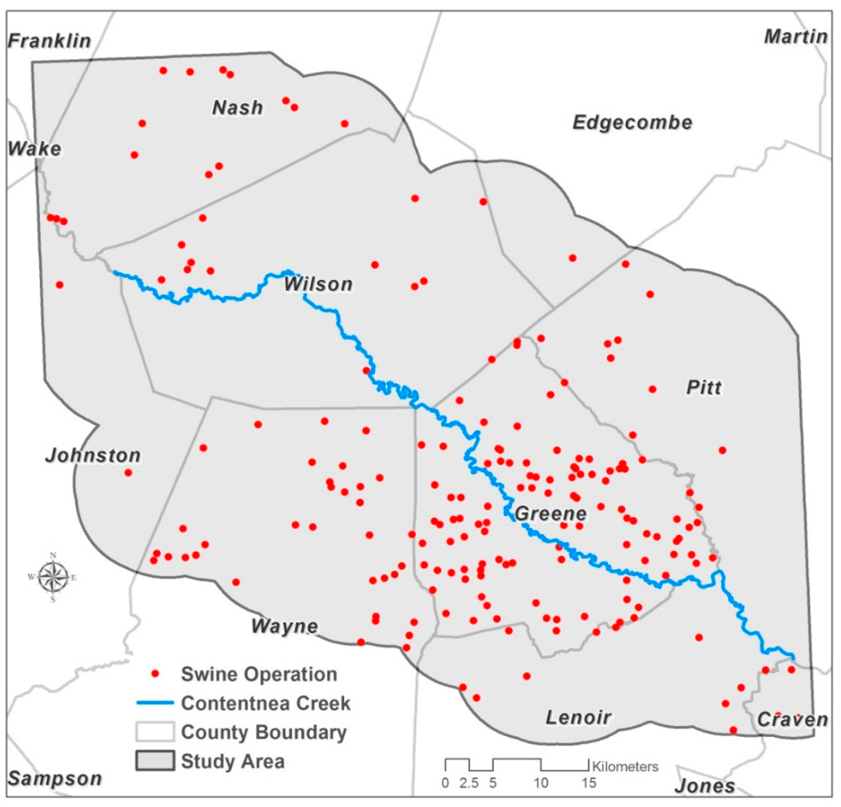
Animal operations data were downloaded online from the NC Department of Environment and Natural Resources (NC DENR) Division of Water Quality website for 2010 (http://portal.ncdenr.org/web/wq/animal-facility-map). The data include the type of animal operation (swine, cattle, poultry and horse), capacity, geographic coordinates, total animal weight in kg and the description of each operation. Latitude/longitude information was used to map 195 swine CAFOs located in our study area (Figure 1).

Our goal was to use a spatial unit of analysis that would allow us to take full advantage of the spatial resolution of the ammonia concentration data (1 km × 1 km pixels) and detailed demographic information; the census block was the best option. We downloaded census block data from the U.S. Census Bureau website for the entire state (census block boundaries, age and racial composition) for 2000 and 2010. Poverty or income data were not included in the analysis, because these data are not publicly available at the census block level.

Both CAFO and census data were projected into the NAD 1983 State Plane North Carolina coordinate system. Census blocks located inside Contentnea Creek Watershed and within five miles outside its boundary were selected for the analysis. Census blocks within urban areas were removed from the analysis because CAFOs are located in rural areas. Boundaries of urban areas were obtained from the Census Bureau (http://www.Census.gov/geo/maps-data/data/cbf/cbf_ua.html). Uninhabited census blocks were excluded, because our focus was on human exposure to air pollution. The final dataset included 3290 census blocks for 2000 and 3685 census blocks for 2010. The number of blocks is different between the two years, because some census boundaries had changed.

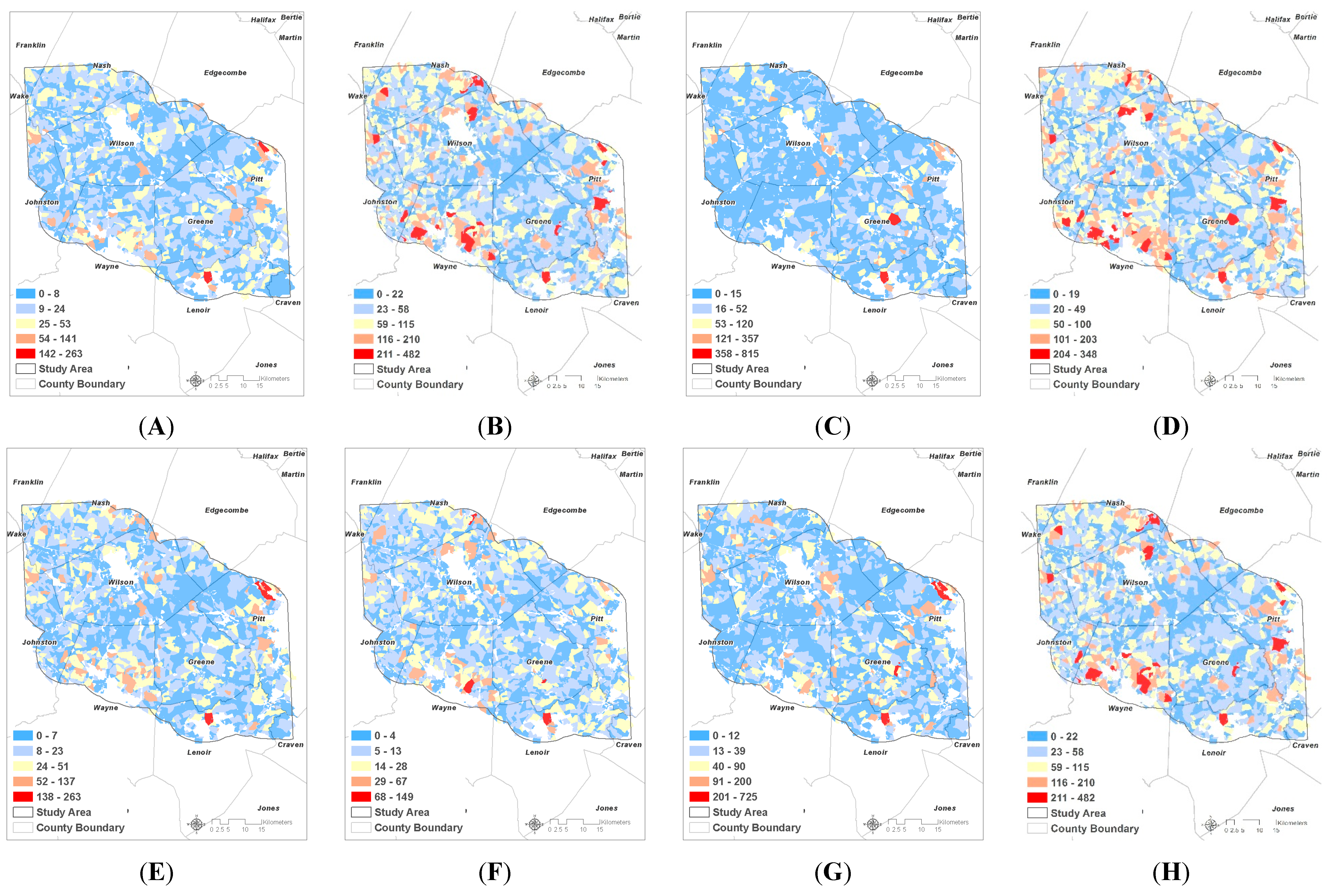
Using 2000 and 2010 U.S. Census data, we calculated the number of people aged 65 and older, the number of people aged 15 and younger and the number of white and minority people. Table 1 shows the demographic data, and Figure 2 shows their spatial distribution. We used the actual number of people within each population group in the environmental justice analysis (instead of percent per census block), because it is a more relevant measure in the context of human exposure to air pollution.

Table 1. Demographic characteristics of census blocks in 2000 and 2010.

Year (# of Census Blocks)	Statistics per Census Block	# of People under 15 Years of Age	# of People over 65 Years of Age	# of Minority Population	# White Population
2000 (3290)	Min	0	0	0	0
	Max	263	93	815	348
	Mean	8	4	12	28
	Median	4	3	3	15
	SD	13	6	29	38
2010 (3685)	Min	0	0	0	0
	Max	263	149	725	482
	Mean	8	5	13	28
	Median	4	3	4	15
	SD	14	7	31	40

Table 1. Demographic characteristics of census blocks in 2000 and 2010.

Year (# of Census Blocks)	Statistics per Census Block	# of People under 15 Years of Age	# of People over 65 Years of Age	# of Minority Population	# White Population
2000 (3290)	Min	0	0	0	0
	Max	263	93	815	348
	Mean	8	4	12	28
	Median	4	3	3	15
	SD	13	6	29	38
2010 (3685)	Min	0	0	0	0
	Max	263	149	725	482
	Mean	8	5	13	28
	Median	4	3	4	15
	SD	14	7	31	40

Figure 2. Demographic variables from 2000 and 2010 Census: (A) population of children under 15 in 2000; (B) population of elderly over 65 in 2000; (C) population of minorities in 2000; (D) population of whites in 2000; (E) population of children under 15 in 2010; (F) population of elderly over 65 in 2010; (G) population of minorities in 2010; (H) population of whites in 2010.

Figure 2. Demographic variables from 2000 and 2010 Census: (A) population of children under 15 in 2000; (B) population of elderly over 65 in 2000; (C) population of minorities in 2000; (D) population of whites in 2000; (E) population of children under 15 in 2010; (F) population of elderly over 65 in 2010; (G) population of minorities in 2010; (H) population of whites in 2010.

4. Methodology

4.1. Modeling Ammonia Concentrations

Air dispersion models have been used to estimate concentrations of pollutants emitted by CAFOs. Some studies modeled the dispersion of odor to define setback distances between CAFOs and residential areas [29]. Other studies attempted to model ammonia and hydrogen sulfide near CAFOs [30,31]. One study used the Industrial Source Complex Short-Term Model, version 3 (ISC-ST3), to model ammonia dispersion and deposition from CAFOs in North Carolina by hydrologic unit and county [30]. This model operates under the assumption that the concentration of the contaminant is defined by a normal, or Gaussian, curve and has some known deficiencies; it does not operate well during stable or near-calm conditions, and it cannot account for the effects of vegetation on concentrations, the effect of elevation nor wind distribution [29].

Another study used the CALPUFF model to model ammonia and hydrogen sulfide emitted by CAFOs in Minnesota [31]. The CALPUFF model accounts for variable wind directions and land cover pattern, includes a calm-wind algorithm and can model dispersion from multiple facilities and over a complex terrain. Due to these advantages, the “U.S. EPA has adopted CALPUFF as the preferred model for assessing long-range transport of pollutants” [29,32].

Following the U.S. EPA’s recommendation [29,32], we selected CALPUFF to model ammonia dispersion in our study. The CALPUFF Modeling System includes three main components: CALMET, CALPUFF and CALPOST. CALMET is a meteorological model that develops wind and temperature models as three-dimensional grids. CALPUFF is a transport and dispersion model that emits “puffs” of material from modeled sources, simulating dispersion and transformation processes along the way. It uses the information generated by CALMET, and temporal and spatial variations in the meteorological grids are explicitly incorporated with the resulting distribution of puffs throughout a simulated period. The output files from CALPUFF contain concentrations evaluated at selected locations, called receptors. CALPOST is used to process these files and produce the summarized results of the simulation [33].

Three main types of data are required to run the model: hourly average meteorological data, facility layout and dimensions and emission data. We purchased meteorological data (MM5 file) from the company that distributes the CALPUFF model (http://www.src.com/calpuff/calpuff1.htm) and used it as input for the CALMET meteorological model. Each MM5 file covers a 120 km × 120 km area and contains a 10 × 10 grid with a spatial resolution of 12 km × 12 km. Our study area (Contentnea Creek Watershed and areas within five miles) is covered by one MM5 file. This grid contains hourly information for an entire year, including wind speed and direction, temperature, relative humidity, pressure, mixing ratios of water vapors, precipitation amount, solar radiation, snow cover, 2-m temperature and specific humidity, 10-m wind speed and direction and sea surface temperature. Only one MM5 file was available for our area of interest and time period, for 2006, so we used it to model ammonia emissions from CAFOs. To check whether 2006 data are representative of weather conditions in the area, we obtained weather observation data for three meteorological stations for 2000–2010: Goldsboro (latitude: 35.37935; longitude: −78.0448), Greenville (latitude: 35.6352389; longitude: −77.3853194) and Rocky Mount (latitude: 35.89295; longitude: −77.67996). Data included monthly average daily temperature, average wind direction, average wind speed and total monthly precipitation. We compared monthly 2006 data with averages for the other 9 years for each station separately (2000–2005; 2006–2010). Our comparisons showed that there was little difference between each month in 2006 and the corresponding values for the other 9 years for this month. For example, wind direction for Greenville was west (265°) in March 2006, and in six out of nine years it had a similar direction (ranging from 219° to 285°). Table 2 shows that there was little difference in wind speed between 2006 and the average for the other 9 years.

Using MM5 data, CALMET calculates 3D wind fields as 1 km × 1 km grids that are used as input for the CALPUFF model.

Table 2. Wind speed (km/hour) averaged for 2000–2005; 2007–2010 and its difference with 2006 wind speed for three meteorological stations in North Carolina [34].

Month	Goldsboro			Greenville			Rocky Mount
	Average	2006	Difference	Average	2006	Difference	Average	2006	Difference
January	5.72	5.31	0.41	3.60	4.35	−0.74	3.92	4.35	−0.42
February	6.37	4.67	1.70	4.20	4.51	−0.30	4.18	4.51	−0.32
March	3.36	4.67	−1.31	2.37	3.54	−1.17	1.97	3.54	−1.57
April	4.05	2.57	1.47	3.38	2.09	1.29	2.96	2.25	0.70
May	3.04	4.02	−0.99	3.02	2.90	0.13	2.92	3.54	−0.62
June	3.04	1.93	1.11	3.54	3.38	0.16	2.72	2.41	0.30
July	3.54	4.02	−0.48	3.38	4.35	−0.97	3.08	3.70	−0.62
August	2.45	1.45	1.01	2.50	1.29	1.22	2.04	1.77	0.27
September	4.87	1.29	3.58	3.38	0.16	3.22	3.50	0.64	2.86
October	3.32	3.22	0.10	1.97	1.77	0.20	1.95	2.09	−0.14
November	3.72	2.90	0.82	2.25	2.09	0.16	2.29	2.09	0.20
December	4.18	1.45	2.74	2.75	1.93	0.82	3.17	1.77	1.39

Table 2. Wind speed (km/hour) averaged for 2000–2005; 2007–2010 and its difference with 2006 wind speed for three meteorological stations in North Carolina [34].

Month	Goldsboro			Greenville			Rocky Mount
	Average	2006	Difference	Average	2006	Difference	Average	2006	Difference
January	5.72	5.31	0.41	3.60	4.35	−0.74	3.92	4.35	−0.42
February	6.37	4.67	1.70	4.20	4.51	−0.30	4.18	4.51	−0.32
March	3.36	4.67	−1.31	2.37	3.54	−1.17	1.97	3.54	−1.57
April	4.05	2.57	1.47	3.38	2.09	1.29	2.96	2.25	0.70
May	3.04	4.02	−0.99	3.02	2.90	0.13	2.92	3.54	−0.62
June	3.04	1.93	1.11	3.54	3.38	0.16	2.72	2.41	0.30
July	3.54	4.02	−0.48	3.38	4.35	−0.97	3.08	3.70	−0.62
August	2.45	1.45	1.01	2.50	1.29	1.22	2.04	1.77	0.27
September	4.87	1.29	3.58	3.38	0.16	3.22	3.50	0.64	2.86
October	3.32	3.22	0.10	1.97	1.77	0.20	1.95	2.09	−0.14
November	3.72	2.90	0.82	2.25	2.09	0.16	2.29	2.09	0.20
December	4.18	1.45	2.74	2.75	1.93	0.82	3.17	1.77	1.39

CAFOs emissions were modeled as area emissions (vs. point or line), because hog houses and lagoons are more accurately represented as areas. We used the following procedure to calculate the dimensions of each operation. First, we randomly selected ten CAFO operations in the area and used Google Earth to draw their boundaries. Then, we calculated the total area of each CAFO (hog houses and lagoons together) and explored the relationship between the total area and the corresponding total weight of animals at each sampled operation. Our calculations showed that, on average, one kg of hog weight takes up about 0.1 m² of CAFO area. Using this conversion factor, we calculated the areal extent of each CAFO operation, representing it as a square of a certain size. Each square was centered on the latitude/longitude coordinates of the corresponding CAFO. Each CAFO’s area size information, along with its elevation above sea level, was put into the CALPUFF model.

Finally, to calculate ammonia emissions from each CAFO, we used ammonia emission rates reported in the literature. A study by Aneja et al. [35] reported that emissions from barns ranged from 0.89 to 1.05 kg-N/week/1000 kg × lm for the cold and warm season, respectively (lm = live animal mass). When recalculated in different units (g/year), these emissions amount to 46.28–54.6 g-N/year/kg live mass. This study also reported ammonia flux rates per minute per square meter of waste lagoon surface. Since we did not have information about the size of each waste lagoon, we could not use the rates reported by this study and instead applied emission rates that were calculated per year per live animal weight or per animal, as reported in a study by Doorn et al. [36]. This study, conducted by the EPA, recommended a general emission factor for hog houses of 59 ± 10 g NH₃/kg live weight/year and for swine lagoons, of 2.4 kg NH₃/year/hog. We multiplied these rates by the corresponding numbers from the CAFOs table (total live weight and the number of hogs at each operation, respectively) and added two emissions together to get the total emissions amount per CAFO per year. We accepted CALPUFF’s default settings and did not model the removal of the ammonia (wet deposition, dry deposition) or its chemical transformation. The output from CALPUFF model was input in CALPOST to produce daily average ammonia concentrations for the entire study area. It was then imported into ArcGIS software as a raster grid with a pixel size of 1 km × 1 km. To calculate the average daily ammonia concentrations per census block, we used the zonal statistics operation in ArcGIS 10.

4.2. Assessing Disproportionate Exposure

To assess disproportionate population exposure to ammonia concentrations, we used techniques of traditional and spatial statistics. First, we calculated the correlation coefficient between ammonia concentrations and each demographic variable for 2000 and 2010. Since North Carolina imposed a CAFO moratorium in 1997–2007, we assumed that the number of CAFOs did not change between 2000 and 2010 and used CALPUFF results for both 2000 and 2010 analyses.

We utilized a Spearman’s correlation coefficient in IBM SPSS Statistics [37] to measure the associations between the average NH₃ concentrations and the specific sociodemographic characteristics of each census block. Spearman’s rank correlation is a nonparametric statistic that first converts the values of the variables to ranks and then calculates the correlations as follows [38]

$$r_s=1-\frac{6{\sum }^{\text{}}{D}^2}{n^3-n}$$

(1)

where:

• r_s = Spearman’s rank correlation coefficient;
• D = the differences between the rank values for each feature on the two variables;
• n = the number of features.

The value of r_s in the result is constrained from 1 (a perfect direct correlation) to −1 (a perfect inverse correlation). The closer r_s is to ±1, the stronger the monotonic relationship, while a r_s near 0 indicates no relationship between the two variables [39].

In order to examine the correlation between ammonia concentrations and sociodemographic variables spatially, a bivariate local indicator of spatial association (LISA) analysis was performed using GeoDa software [40]. Developed by Luc Anselin [41], a local indicator of spatial association, also known as a univariate LISA, tests whether local correlations between values of a feature and values of its neighbors are significantly different from what would be expected from a complete spatial randomization. It identifies significant spatial clusters by involving the cross product between the standardized value of a variable for feature i  and that of the average of the neighboring values:

$$I_i=\frac{x_i-\overline{X}}{S_i^2}{\displaystyle \sum }_{j=1,j\ne i}^n{\omega }_{i,j}\left(x_j-\overline{X}\right)$$

(2)

where:

• x_i = an attribute value for feature i;
• $\overline{X}$ = the mean of the corresponding attribute;
• w_i,j = the spatial weight between features i and j, and:

  $$S_i^2=\frac{{{\displaystyle \sum }}_{j=1,j\ne i}^n{\left(x_j-\overline{X}\right)}^2}{n-1}-{\overline{X}}^2$$

  (3)

  n = the total number of features.

As a simple extension of the univariate LISA, the bivariate LISA identifies the extent of spatial clusters by involving the cross product of the standardized values of one variable at location i with that of the average neighboring values of the other variable. The statistical significance of these spatial clusters is evaluated using Monte-Carlo spatial randomization [41].

Bivariate LISA produces four clusters: high-high, high-low, low-high and low-low. In the context of our study, a high-high cluster indicates areas with a higher than average concentration of ammonia surrounded by neighbors with more than the average number of people from a vulnerable population group (children, the elderly, whites or minorities). A high-low cluster indicates areas with a higher than average concentration of ammonia surrounded by neighbors with less than the average number of people from a vulnerable population group. A low-high cluster indicates areas with a lower than average concentration of ammonia surrounded by neighbors with more than the average number of people from a vulnerable population group, and a low-low cluster indicates areas with a lower than average concentration of ammonia surrounded by neighbors with less than the average number of people from a vulnerable population group.

To conduct the LISA analysis, a weights matrix is created to conceptualize the spatial relationships. Considering that the areal units are irregular, this study used a distance-based spatial weight matrix, selecting polygons located within a particular distance as neighbors of the target polygon. Since this particular distance is an important parameter for modeling spatial relationships, we selected an appropriate distance threshold with the assistance of the Incremental Spatial Autocorrelation tool in ArcGIS. Specifically, this tool examines spatial autocorrelation at various distances and provides the associated z-scores reflecting the intensity of spatial clustering [42]. The distance associated with the highest z-score is chosen as the threshold distance for the weight matrix. Incremental Spatial Autocorrelation identified 4 kilometers as the distance that resulted in the highest z-score, so we used it as the threshold for the calculation of the spatial weights matrices for both 2000 and 2010.

5. Results

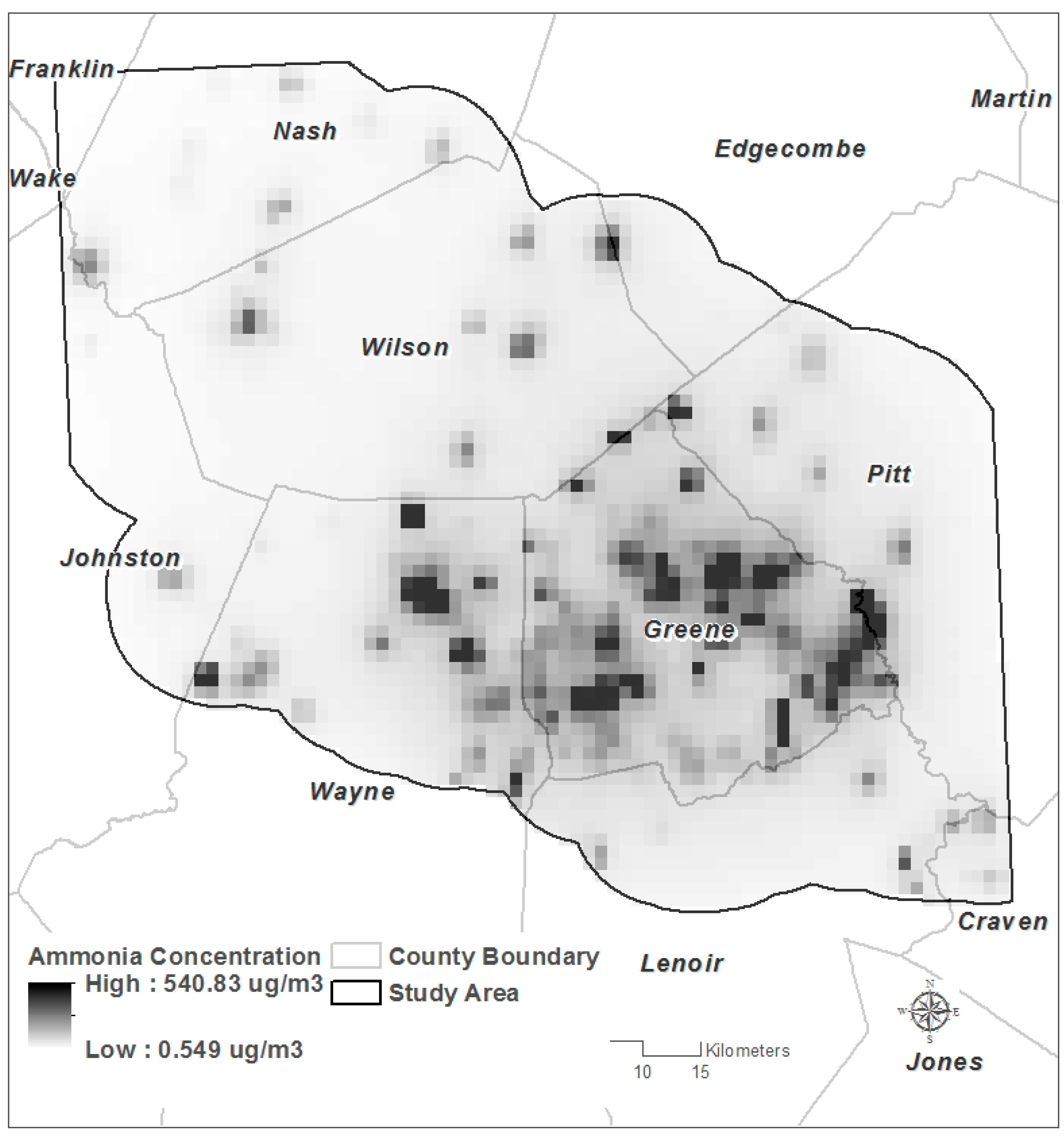
The raster grid of modeled ammonia concentrations is shown in Figure 3. The average modeled concentration is 14.773 µg/m³, (min = 0.549; max = 540.837 µg/m³). The maximum value is observed in areas where multiple CAFOs are located next to each other, mostly in Green County. To validate our model, we compared our results with a study by Wilson and Serre [43], who used passive samplers to measure ammonia in eastern North Carolina. They found that, at sites within 2 km from a hog CAFO, the ammonia concentration averaged 19.872 µg/m³, reaching as high as 115.2 µg/m³. While these measurements are very similar to our modeled concentrations, it is important to note that we only modeled emissions from swine CAFOs and did not account for other sources of ammonia. According to Battye et al. [44], livestock waste accounts for about 80% of ammonia emissions in North Carolina, and other sources include fertilizer application, forests, non-agricultural vegetation and motor vehicles.

Figure 3. CALPUFF output: modeled ammonia concentrations (µg/m³).

Figure 3. CALPUFF output: modeled ammonia concentrations (µg/m³).

We also compared our results with concentrations measured at an Ambient Ammonia Monitoring Network (AMoN; http://nadp.sws.uiuc.edu/amon/) site located about 50 km outside our study area (Clinton Crops Research Station; latitude 35.0258; longitude −78.2783). This AMoN site is the closest to our study area. Based on biweekly samples from February 2009 to February 2010, ammonia concentrations at this site ranged from 1.11 to 8.3 µg/m³, with a mean concentration of 4.191 µg/m³. These measurements are comparable to our modeled concentrations (mean values of 4.191 vs. 14.773 µg/m³, respectively). Lower values at the monitoring station could be explained by the fact that it is located 1.4 km from the nearest CAFO, while our model predicts concentrations for the entire study area, including areas in the immediate vicinity of CAFOs.

The Spearman’s correlation between the average ammonia concentrations and each demographic variable for 2000 and 2010 is shown in Table 3. In 2000, statistically significant, but weak, relationships were identified between the average ammonia concentration and three demographic variables. Specifically, population under 15 years of age and minority population have a significant positive correlation with the ammonia concentration at the 99% confidence level; population over 65 years of age and the ammonia concentration are significantly correlated at the 95% confidence level. However, in 2010 only, minority population had a significant, but weak, positive correlation with the average concentration of ammonia. No significant relationship was found for the other three variables.

Table 3. Spearman’s rank correlation coefficients (* p < 0.05; ** p < 0.01).

Year	Demographic Variable	Ammonia Concentration
2000 Census Data	Under 15 years of age	0.046 **
	Over 65 years of age	0.038 *
	Minority population	0.162 **
	White population	−0.034
2010 Census Data	Under 15 years of age	0.024
	Over 65 years of age	0.008
	Minority population	0.104 **
	White population	−0.031

Table 3. Spearman’s rank correlation coefficients (* p < 0.05; ** p < 0.01).

Year	Demographic Variable	Ammonia Concentration
2000 Census Data	Under 15 years of age	0.046 **
	Over 65 years of age	0.038 *
	Minority population	0.162 **
	White population	−0.034
2010 Census Data	Under 15 years of age	0.024
	Over 65 years of age	0.008
	Minority population	0.104 **
	White population	−0.031

Bivariate LISA examined the correlation between the ammonia exposure and demographics and identified significant spatial clusters (p = 0.05). For the purposes of this study, we focus our attention on high-high clusters, because they represent areas where high numbers of vulnerable people are exposed to higher than the average level of pollutant concentrations. These high-high clusters are also often referred to as “hot spots”. We calculated the average ammonia concentrations in hot spots for 2000 and 2010 and compared them with ammonia concentrations for the whole study area (Table 4). Our calculations show that average ammonia concentrations in hot spots for 2000 and 2010 are 2.5–3-times higher than the average concentration in the entire watershed. Figure 4, Figure 5, Figure 6 and Figure 7 show the locations of high-high clusters for both years for four vulnerable population groups.

Table 4. Statistics for ammonia concentrations (µg/m³) in the entire study area and in the 2000 and 2010 hot spots for minorities, whites, children (under 15 years old) and the elderly (over 65 years old).

Statistics	Entire Study Area	2000 Hot Spots				2010 Hot Spots
		Non-White	White	Under 15	Over 65	Non-White	White	Under 15	Over 65
Min	0	14	4	14	14	14	6	14	0
Max	530	316	530	530	138	87	530	530	530
Mean	12	37	34	33	30	34	32	32	31

Table 4. Statistics for ammonia concentrations (µg/m³) in the entire study area and in the 2000 and 2010 hot spots for minorities, whites, children (under 15 years old) and the elderly (over 65 years old).

Statistics	Entire Study Area	2000 Hot Spots				2010 Hot Spots
		Non-White	White	Under 15	Over 65	Non-White	White	Under 15	Over 65
Min	0	14	4	14	14	14	6	14	0
Max	530	316	530	530	138	87	530	530	530
Mean	12	37	34	33	30	34	32	32	31

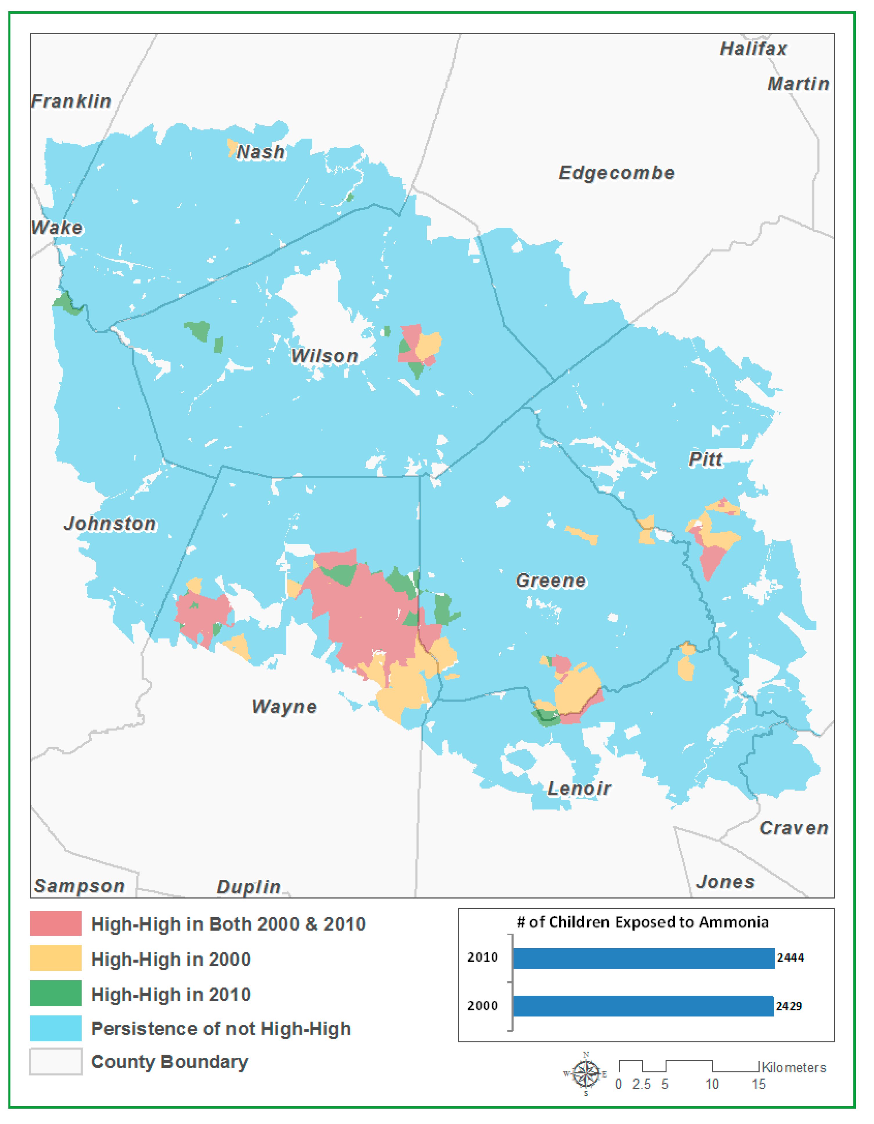
In both years, high-high clusters indicating a high ammonia concentration and a high population under 15 years of age are mainly located in Wayne County, close to the boundary of Greene County. Several small clusters can also be found in Greene, Lenoir and Pitt counties. In 2000, 148 census blocks were included in high-high clusters; in 2010, that number increased to 160. This change is also reflected in the number of children who lived in these hot spots: it increased by 15 children.

Figure 4. Bivariate local indicator of spatial association (LISA) hot spots in 2000 and 2010: average ammonia concentration with population under 15.

Figure 4. Bivariate local indicator of spatial association (LISA) hot spots in 2000 and 2010: average ammonia concentration with population under 15.

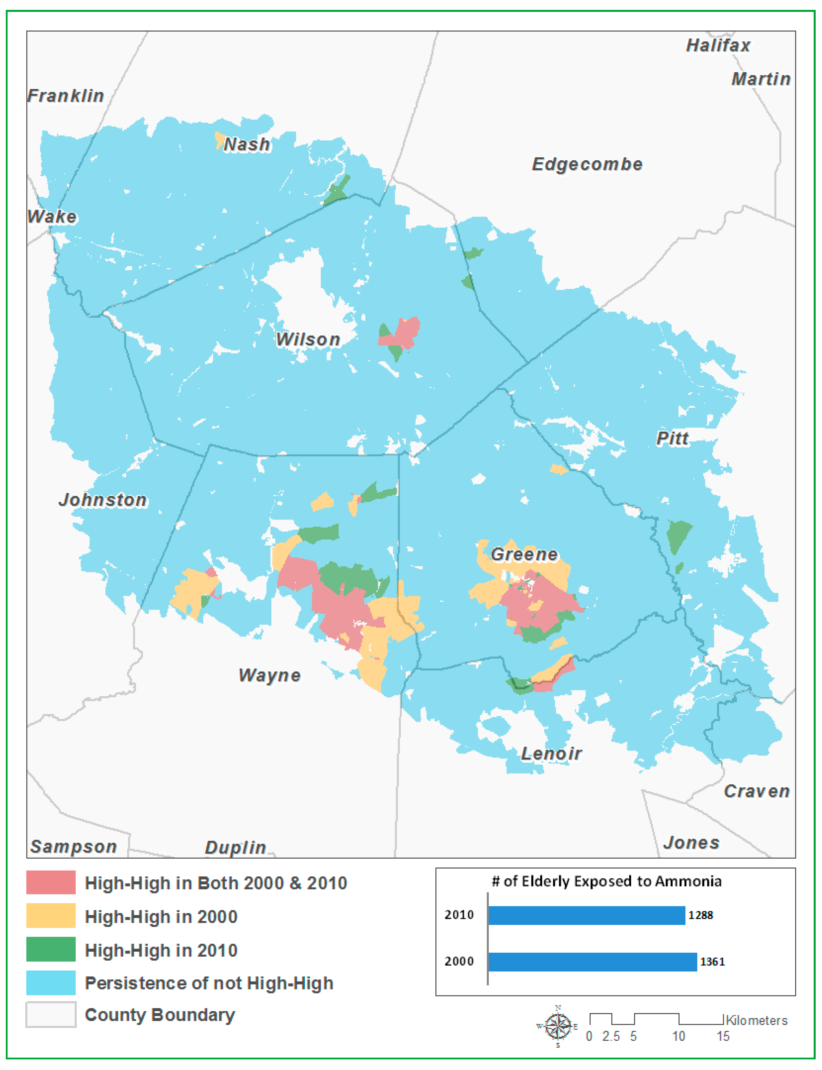
When analyzing the spatial association between ammonia concentration and population over 65 years of age, large high-high clusters for both years can be found in Wayne and Greene counties. In 2000, 190 census blocks were included in high-high clusters; in 2010, that number was 189. The number of elderly living in hot spots decreased by 73 people between 2000 and 2010.

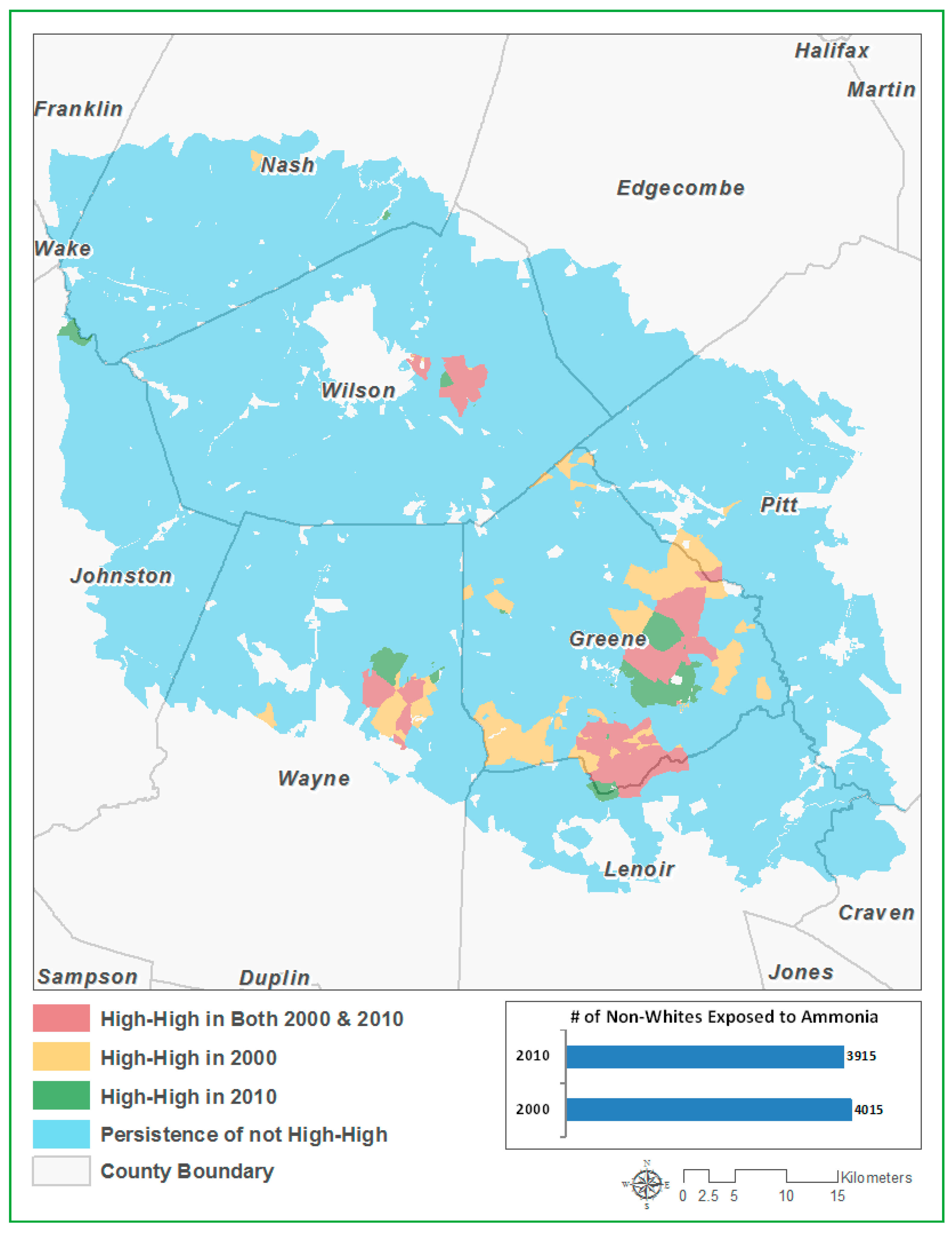
A different pattern is observed for minority population, and most of the high-high areas showing persistence in both years are located in Greene County. Wayne and Wilson Counties also contain a small number of high-high clusters in both years. In 2000, 188 census blocks were included in high-high clusters; in 2010, that number decreased to 124. One hundred fewer minority people were living in these hot spots in 2010 as compared to 2000.

Figure 5. Bivariate LISA hot spots in 2000 and 2010: average ammonia concentration with population over 65.

Figure 5. Bivariate LISA hot spots in 2000 and 2010: average ammonia concentration with population over 65.

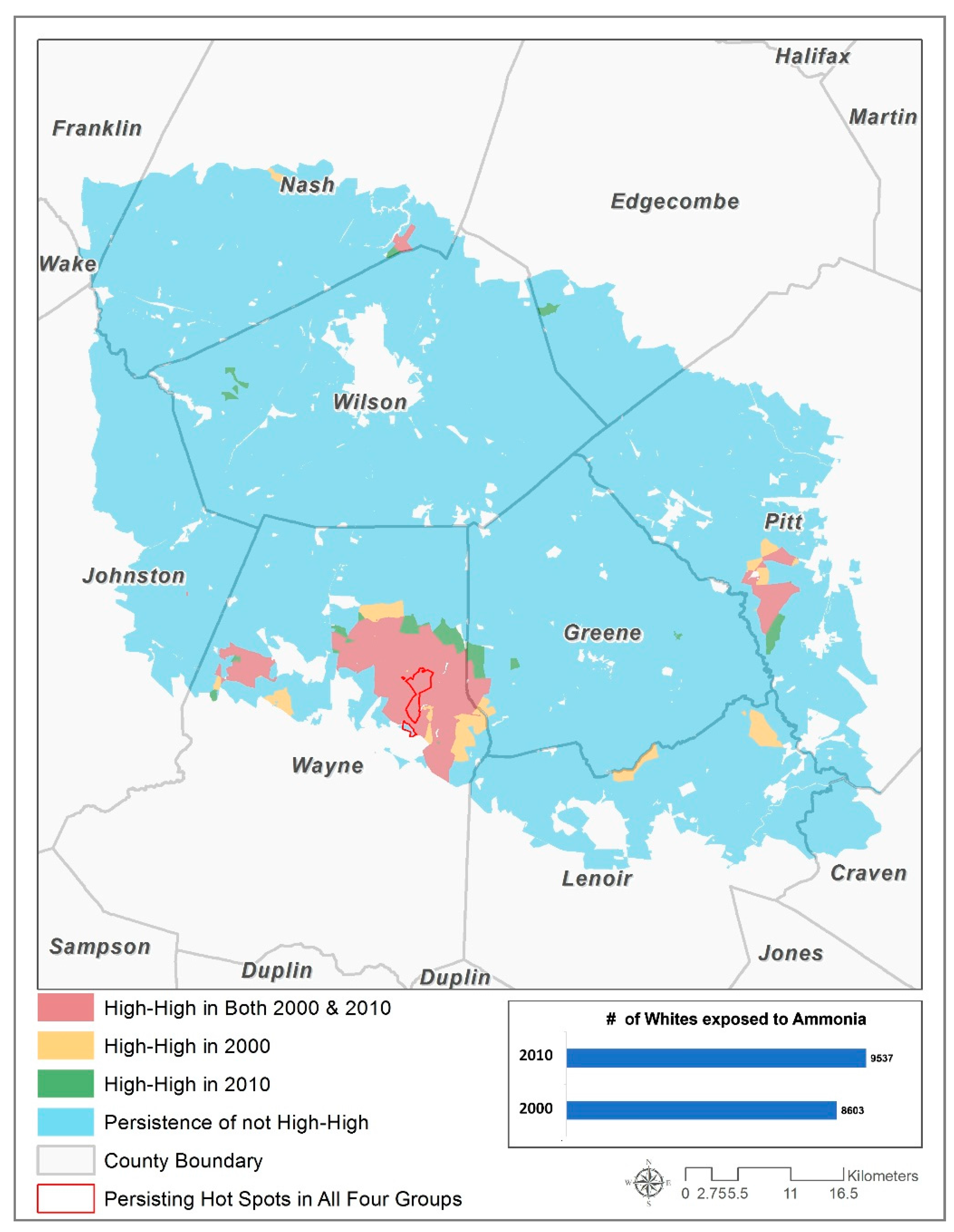
In both years, high-high clusters indicating a high ammonia concentration and high white population are mainly located in Wayne and Pitt Counties. In 2000, 132 census blocks were included in high-high clusters; in 2010, that number increased to 182. The number of white people who lived in these hot spots increased by 934.

Figure 6. Bivariate LISA hot spots in 2000 and 2010: average ammonia concentration vs. population of minorities.

Figure 6. Bivariate LISA hot spots in 2000 and 2010: average ammonia concentration vs. population of minorities.

To compare the spatial locations of persisting hot spots of four vulnerable populations, we overlaid four maps. Spatial coincidence analysis showed 12 census blocks that belonged to a persisting hot spot in all four maps (Figure 7). These areas are located in Wayne County and represent an extreme case of potential environmental injustice, where disproportionately high numbers of children, elderly, whites and minorities could have been exposed to high ammonia concentrations in 2000 and 2010.

Figure 7. Bivariate LISA hot spots in 2000 and 2010: average ammonia concentration vs. population of whites and persisting hot spots of all four population groups.

Figure 7. Bivariate LISA hot spots in 2000 and 2010: average ammonia concentration vs. population of whites and persisting hot spots of all four population groups.

6. Discussion and Conclusions

The main research question of this study asked if children, the elderly, white and minority populations are disproportionately exposed to ammonia emitted by CAFOs in Contentnea Creek Watershed in North Carolina. To answer this question, the study used the CALPUFF software to model ammonia emission and dispersion from CAFOs and applied the Spearman correlation and LISA analysis to examine the relationship between ammonia concentrations and demographic characteristics in 2000 and 2010.

The CALPUFF model used very detailed data about meteorological conditions and the characteristics of CAFO facilities (location, dimensions and ammonia emissions per hog or kg of live weight) to produce ammonia emission estimates as a continuous surface with 1-km² pixels. The fine spatial scale of the modeled ammonia output matched the spatial dimensions of census data very well: the average census block in the study areas is 0.78 km². Areas with the highest concentration of ammonia were found in Greene County and Wayne County, where the concentration of CAFOs is the highest.

The Spearman’s correlation analysis showed that a weak positive relationship existed between average ammonia concentration and some of the demographic variables. Most of the correlation coefficients were statistically significant, probably due to the large sample size (the number of census blocks in each year was over 3000). While these findings indicate that higher numbers of vulnerable people are associated with higher ammonia concentrations in the area, they do not provide any insight into the spatial pattern of these relationships.

Bivariate LISA analysis identified hot spots of environmental injustice: areas with high ammonia concentrations are surrounded by areas with high numbers of vulnerable population. Although the population in three vulnerable groups within hot spots has slightly decreased between the two years, the number of people disproportionately exposed to ammonia concentrations was still large in 2010: 2444 children, 1288 elderly people, 9537 whites and 3915 minorities.

Using spatial overlay in GIS, we identified areas that could have experienced an extreme case of environmental injustice, because they were included in hot spots for all four population groups in both years. A spatial query showed that just within three miles from these areas, there were 12 CAFOs. The results of air pollution modeling suggest that these areas should be prioritized for ambient air quality monitoring.

It is beneficial to discuss these findings in the context of existing air quality regulations. Unfortunately, there is no federal-level standard regarding ammonia, because it is not one of the six criteria air pollutants covered by the Clean Air Act (http://scorecard.goodguide.com/env-releases/def/cap_naaqs.html). EPA requires some CAFOs to report estimated ammonia and hydrogen sulfide emissions based on the number of confined animals. For example, swine CAFOs that have more than 2500 swine, each weighing 55 pounds or more, or 10000 swine, each weighing less than 55 pounds, are required to report their emission estimates (http://www.ecy.wa.gov/epcra/CERCLA_CAFOairexempt.pdf). The Occupational Safety and Health Administration (OSHA) has set an acceptable eight-hour exposure and a short-term (15 min) exposure level for ammonia (http://www.atsdr.cdc.gov/toxfaqs/tf.asp?id=10&tid=2), but these standards mainly concern CAFO workers and are not directly applicable to the general population living in the area. State-level air quality regulations vary, and the majority of states do not have a comprehensive air quality regulatory system. For example, Missouri has an ambient acceptable level of ammonia, and North Carolina and Colorado have regulations concerning odor emissions from CAFOs, but no emission standards for hydrogen sulfide or ammonia [45].

The Agency for Toxic Substances and Disease Registry (ATSDR) includes ammonia in its toxic substances list and provides minimal risk level concentrations for it. According to the ATSDR, the minimal risk level (MRL) “is an estimate of the daily human exposure to a hazardous substance that is likely to be without appreciable risk of adverse, non-cancer health effects over a specified duration of exposure. The information in this MRL serves as a screening tool to help public health professionals decide where to look more closely to evaluate possible risk of adverse health effects from human exposure.” (http://www.atsdr.cdc.gov/mrls/index.asp). Ammonia’s MRL for chronic exposure (meaning exposure for one year or longer) is set at 0.1 ppm, or 75 µg/m³ (http://www.atsdr.cdc.gov/mrls/mrllist.asp#2tag). Applying this threshold to our modeled concentrations, we identified areas where chronic exposure exceeds MRL. Most of these areas overlap with our identified hot spots and correspond to high CAFO density areas in Greene and Wayne Counties. While the spatial extent of these areas is small (2.5% of the watershed), they correspond to densely populated areas with total population ranging from 3647 people in 2000 to 3360 people in 2010. Following ATSDR’s suggestion, these areas deserve further attention of public health professionals to examine possible adverse health effects due to chronic exposure to higher than the minimal risk levels of ammonia.

This study contributes to the body of research on CAFOs and environmental justice, because no other study has yet analyzed environmental justice on the basis of unequal exposure to CAFO-related emissions. Previous environmental justice studies of CAFOs used proximity to CAFOs or their density as the proxy for air pollution exposure. Our study is the first one to directly link modeled pollutant concentrations and demographic characteristics. The proposed methodology is also the first one of its kind to analyze CAFOs-related environmental justice at the finest possible spatial scale, the census block. Previous studies conducted their analysis at the county, census track or census block group levels.

Our study also contributes to a broader literature on environmental justice. Traditionally, environmental justice research has analyzed unequal exposure in the context of race and poverty; including age-based vulnerable population groups in the analysis is an advantage of our study. Both children and elderly are recognized as the most vulnerable age groups, but they are rarely included in environmental justice studies.

There are several limitations to this study, mostly associated with the CALPUFF model and data availability. First, to run the CALPUFF model, we needed very detailed meteorological data, and the only available data compatible with CALPUFF was for 2006. Therefore, we assumed that the 2006 meteorological data represents the average meteorological situation and used CALPUFF output based on 2006 to analyze environmental justice in 2000 and 2010. Since the entire year of data was used to model average daily ammonia concentrations, this assumption seems reasonable. The second limitation relates to CALPUFF model parameters (for example, the user’s choice for background pollution concentrations, the incorporation of wet and dry deposition or the choice of chemical conversion mechanism). We accepted the default settings within the model, and future studies should assess the sensitivity of modeling results to these parameter settings. The third limitation is related to CAFO data availability, including the type and individual size of manure storage facilities. We used 2010 CAFO data to analyze unequal exposure in 2000 and 2010, assuming that the CAFO size did not change during this time to an extent that it would have an effect on the modeled ammonia concentrations. We also did not have data on the type of facility (breeder versus finisher facility) nor the management practices and assumed that the emissions rate is the same for all facilities and remains constant thought the year.

Another limitation of this study is that our findings are only valid at the census block level and cannot be extrapolated to other spatial scales. The reason for that is that the relationships between hazardous facilities and socioeconomic variables may change or become more or less significant when the spatial scale changes [46]. This issue is often referred to as the modifiable area unit problem [47].

Our modeled ammonia concentration was comparable to ammonia concentrations measured in the field by other researchers [43] and by the Ambient Ammonia Monitoring Network. In the future, it would be important to test other atmospheric dispersion models and to compare their results with CALPUFF and field measurement for various pollutants and different geographical regions. These studies should include up-to-date characteristics of polluting facilities, such as individual CAFO operations (e.g., exact size of animal houses and lagoons, number of animals, total animal weight). More studies of this kind (based on pollution dispersion models and using reliable fine-scale demographic data) will allow one to assess the impacts of the CAFOs and to address the concerns regarding the health and quality of life of vulnerable populations.