Habitat Mapping and Change Assessment of Coastal Environments: An Examination of WorldView-2, QuickBird, and IKONOS Satellite Imagery and Airborne LiDAR for Mapping Barrier Island Habitats

Abstract

Habitat mapping can be accomplished using many techniques and types of data. There are pros and cons for each technique and dataset, therefore, the goal of this project was to investigate the capabilities of new satellite sensor technology and to assess map accuracy for a variety of image classification techniques based on hundreds of field-work sites. The study area was Masonboro Island, an undeveloped area in coastal North Carolina, USA. Using the best map results, a habitat change assessment was conducted between 2002 and 2010. WorldView-2, QuickBird, and IKONOS satellite sensors were tested using unsupervised and supervised methods using a variety of spectral band combinations. Light Detection and Ranging (LiDAR) elevation and texture data pan-sharpening, and spatial filtering were also tested. In total, 200 maps were generated and results indicated that WorldView-2 was consistently more accurate than QuickBird and IKONOS. Supervised maps were more accurate than unsupervised in 80% of the maps. Pan-sharpening the images did not consistently improve map accuracy but using a majority filter generally increased map accuracy. During the relatively short eight-year period, 20% of the coastal study area changed with intertidal marsh experiencing the most change. Smaller habitat classes changed substantially as well. For example, 84% of upland scrub-shrub experienced change. These results document the dynamic nature of coastal habitats, validate the use of the relatively new Worldview-2 sensor, and may be used to guide future coastal habitat mapping.

1. Introduction

Barrier islands exist along much of the coastline along the Eastern United States, and are home to many species of flora and fauna. These areas are constantly undergoing geomorphic change due to wind and water stresses that alter their size and orientation [1,2]. This study used remote sensing and GIS technology to assess how Masonboro Island, a National Estuarine Research Reserve System (NERRS) site in North Carolina, USA, has changed, in terms of habitat land cover, over an eight-year period (2002 to 2010). To study habitat change, WorldView-2, QuickBird, and IKONOS satellite imagery and Light Detection and Ranging (LiDAR) elevation and texture data were tested for mapping the study area. The primary objectives of this study were to determine the accuracy of several different satellite sensors and image processing methods for mapping coastal vegetation and to assess how the island has changed over time. The results may help management officials and policy makers enact appropriate preservation measures to mitigate future change and prepare for anticipated habitat loss. The methodologies developed can also be implemented to study other coastal locations.

1.1. Barrier Island Geomorphology

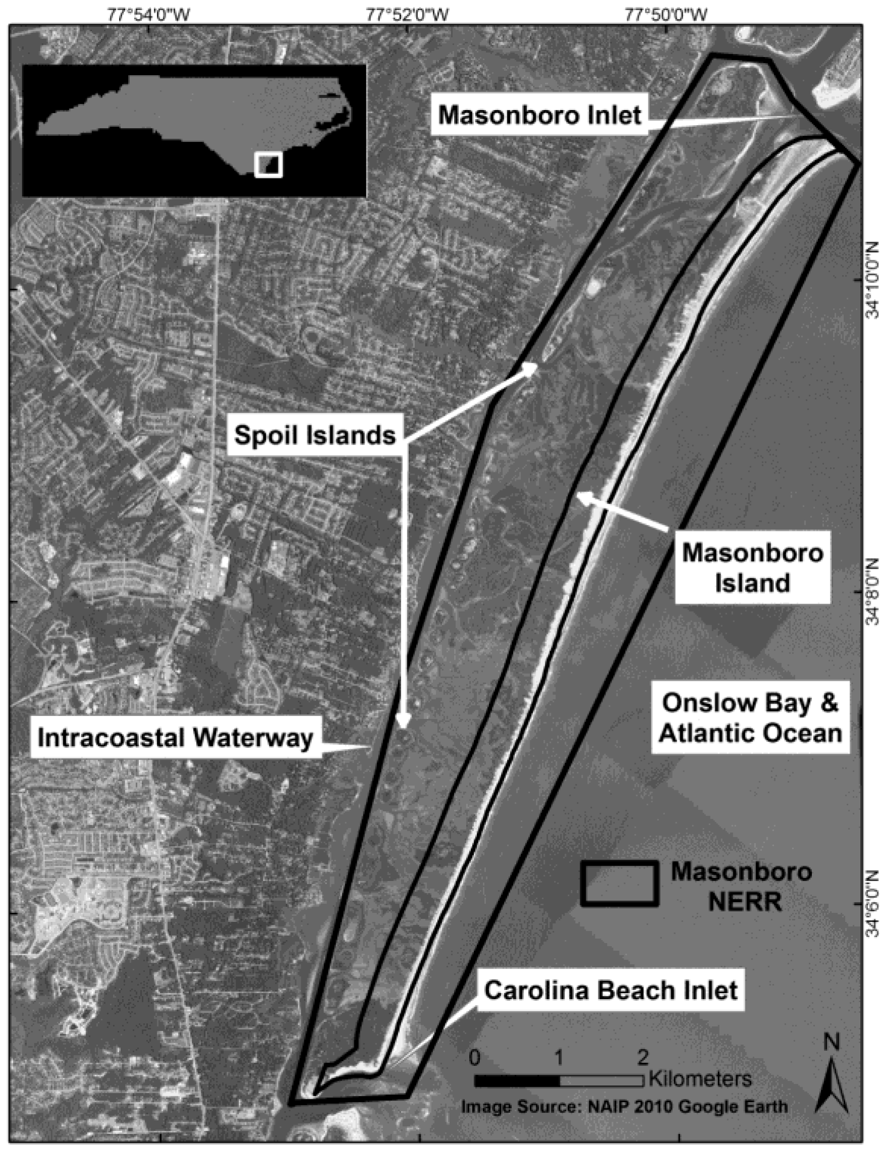
Virtually every area of a barrier island system is continuously vulnerable to geomorphic change, and many of these areas provide, or have the potential to provide, suitable substrate to recruit vegetation. These areas include the supratidal beach, dune ridge systems, saltmarsh, tidal flats, and dredge spoil islands. Barrier islands are very dynamic environments. Erosion, accretion, fragmentation, island migration, storm overwash, and inlet migration are the primary forms of geomorphic change that influence the islands to varying degrees depending on weather conditions, island size and orientation, local sediment budgets, and a number of other factors [1,3]. Loss of stabilizing vegetation may lead to increased erosion [4].

The United States has 405 barrier islands that represent 24% of global barrier islands in terms of total island length, both developed and undeveloped, and many of these could benefit from a standardized, cost- and time-efficient habitat mapping methodology [5]. Changes will occur in coastal locations, which make documenting high-resolution habitat change over time helpful for quantifying the geomorphic evolution and for conservation efforts to be implemented more effectively.

Barrier island geomorphologic evolution is closely tied to its vegetation. Dune plant species promote sediment deposition, which shapes dune systems. Dune systems, in turn, influence sediment mobility, the spatial distribution of topographic differences, and affect the distribution of vegetation cover. Studies of coastal dune vegetation have determined that salt spray exposure, sediment mobility, and soil moisture are the primary factors influencing dune vegetation [6]. The NERRS Habitat and Land Cover Classification Scheme uses these factors, among others, in its hierarchical habitat descriptions [7]. By studying vegetation spatial patterns over time, island morphodynamics may become easier to predict for future conservation efforts.

1.2. Study Area

Masonboro Island NERRS (Figure 1) is an approximately 13 km long, 20.4 square kilometer undeveloped barrier island in southeastern North Carolina. Despite protection from significant anthropogenic degradation, the island is subject to constant change because of the dynamic nature of barrier islands. The island consists of more than 6 km² of salt marsh, and, yet, the majority of research conducted to date has focused on the supratidal beach and upland dune areas as opposed to the entire NERRS as a whole. The North Carolina NERRS site profile [4] contains pertinent information about the study area, but acknowledges a lack of information regarding marsh change through time, such as accretion, erosion, and fragmentation.

Figure 1. Masonboro Island National Estuarine Research Reserve is an undeveloped and protected area off the coast of Wilmington, North Carolina, USA.

Figure 1. Masonboro Island National Estuarine Research Reserve is an undeveloped and protected area off the coast of Wilmington, North Carolina, USA.

Dredge spoil islands are some of the more prominent and stable features of the study area. The US Army Corps of Engineers has been dredging the Intracoastal Waterway and nearby inlets along Southeastern North Carolina since the 1920s and depositing the resulting sediment in discrete areas along the backs of many barrier islands, among other locations [4]. These landmark structures are anthropogenic in origin, but have become incorporated into the back-barrier ecosystem. They can provide substrate for much of the area’s upland vegetation that can be recruited to these islands at different elevations according to individual sunlight, nutrient, and water requirements [8]. The quantity of sediment and length of time that dredging took place has built many of these islands to significant elevations that often exceed natural elevations. Despite the ecological significance, these spoil islands, as well as the adjacent saltwater marshes, have been sparsely studied, but are an important component of the Masonboro Island NERRS study area. These dredge spoil islands dot the landward boundary of Masonboro Island along the Intracoastal Waterway, while Onslow Bay and the Atlantic Ocean lie to the east. The island was separated from Carolina Beach to the south in 1952 with the opening of Carolina Beach Inlet. Masonboro Inlet forms the northern boundary and has been stabilized by a rock jetty since 1981.

One of the more pervasive problems affecting all North Carolina (NC) NERRS sites is invasive species. Masonboro Island is known to have Beach Vitex (Vitex rotundifolia) and Common Reed (Phragmites australis). The former has been found and removed in the past, but is expected to become a more significant problem in the future. The latter species is found on several spoil islands in large monocultures and is known to replace native marsh plants by altering the soil biochemistry and reducing waterfowl usage of the area [9]. Among other plants that need to be monitored, Seabeach Amaranth (Amaranthus pumilus), and Dune Bluecurls (Trichostemasp) are listed as threatened and significantly rare species, respectively [4]. Monitoring these species through island-wide mapping will help management officials assess their abundance and distribution, and help decide if further action needs to be taken to preserve or remove vegetation [10,11].

1.3. Coastal Remote Sensing

Reserve management decision-makers require up-to-date spatial data and quantitative analysis of dynamic barrier island processes in order to implement strategies to maintain and conserve the islands. Monitoring and assessing changing environments can be done using a variety of methods. Many traditional approaches, including field sampling and surveying, require time-consuming and costly efforts with teams of investigators [12]. Use of technological advances in remote sensing data and techniques has revolutionized mapping efficiency, especially in remote locations. In coastal and wetland locations, in particular, remote sensing techniques have been useful for environmental, socio-economic, and anthropogenic land-use assessment [13,14,15,16]. Therefore, the proven potential of this technology dictates the usefulness for continuous improvement in accuracy, precision, and efficient use of time and money.

Although coastal habitat mapping using satellite imagery has been successful, there have been documented issues with reduced map accuracy when mapping Spartina as lower plant density can expose a significant amount of soil and water visible to a remote sensor [17]. The spectral signature of the microphytobenthos contained in the soil may confuse the classification because of the significant quantities of chlorophyll. This can lead to overestimation of Spartina in the lowest areas of the marsh, where Spartina and bare soil areas typically occur.

Zhou et al. [12] emphasized the need for regular monitoring and change detection assessment of wetlands for their protection. They encourage remote sensing of these areas because of the synoptic and repetitive abilities of aerial and orbital sensors, as well as the promising development of new sensors with improved spatial and spectral resolutions. Their classifications of urban wetlands in China were successfully conducted using IKONOS satellite images due to the high spatial resolution afforded by this sensor (4 m unsharpened; 1 m pan-sharpened).

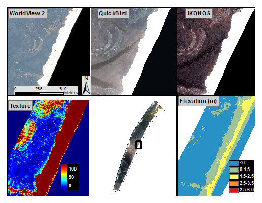
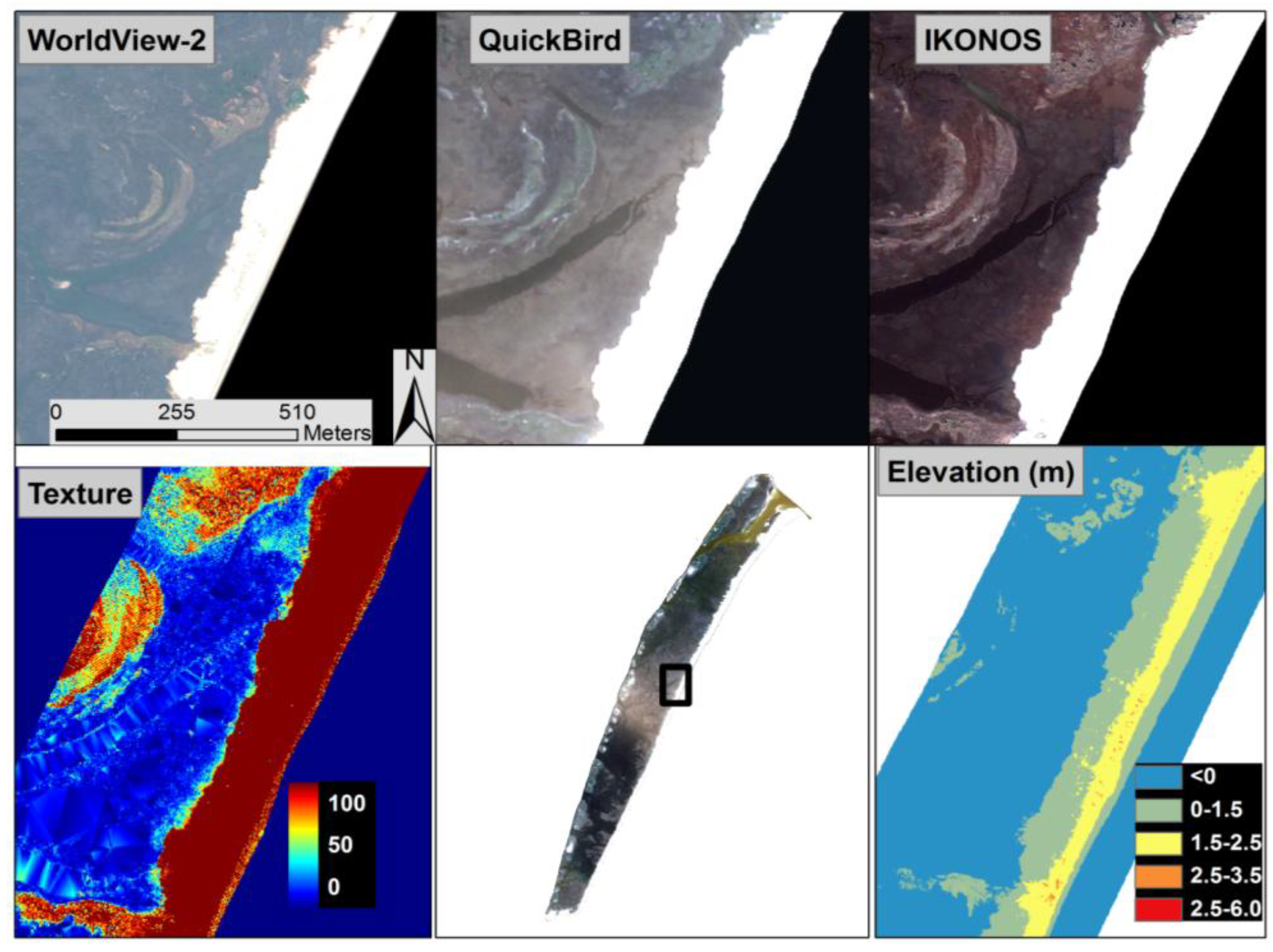
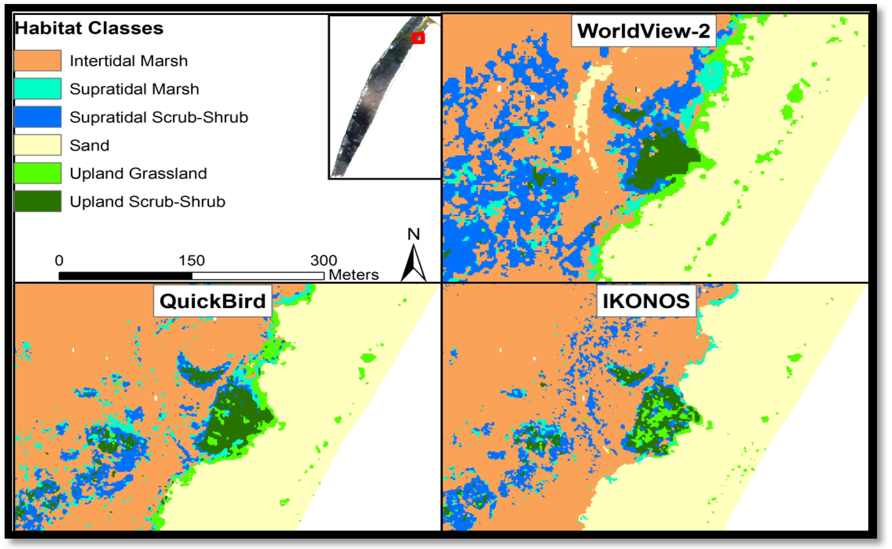
1.4. WorldView-2 Satellite Imagery

DigitalGlobe launched the WorldView-2 (WV-2) satellite in 2010 (Figure 2). WV-2 has a spatial resolution of 1.84 m, eight spectral bands, and the ability to pan-sharpen the imagery to 0.5 m spatial resolution [18]. WV-2 collects images with 11 bits of dynamic range, which are then stored as 16-bit integers. This radiometric resolution enables the sensor to distinguish slight differences in reflected or emitted energy, which may prove valuable for mapping coastal vegetation with similar spectral reflectance patterns. The blue, green, red, and near infrared-1 bands are comparable to those of QuickBird and IKONOS, but the four new bands are unique and potentially useful for mapping coastal habitats (Table 1).

Figure 2. Natural color images and LiDAR texture and elevation for a selected region of Masonboro Island, NC, USA.

Figure 2. Natural color images and LiDAR texture and elevation for a selected region of Masonboro Island, NC, USA.

1.5. QuickBird and IKONOS Satellite Imagery

DigitalGlobe launched the QuickBird (QB) satellite sensor in October 2001, as the first of its high spatial resolution commercial imagery satellites. It has been imaging the Earth for over a decade with four multispectral bands at 2.4 m spatial resolution and a panchromatic band at 0.65 m. QB was selected for this study because of the high spatial resolution and proven usefulness in vegetation mapping, including coastal and wetland classification [10,17,19,20,21,22]. However, QB lacks adequate spectral resolution to map species-specific marsh vegetation but is useful in areas that are unaltered by human activity [17].

Space Imaging (now owned by GeoEye) launched the IKONOS (IK) satellite in September 1999 [23]. IK features the same four multispectral bands as QB over a range, but the individual band ranges differ (see Table 1). IK has a multi-spectral spatial resolution of 4 m, but may be pan-sharpened to 1 m. IK and QB have been used to classify five species of saltmarsh vegetation, as well as soil and water around Venice Lagoon, Italy [14]. Unsupervised and supervised classifications were run on each image, which were then assessed for accuracy using in situ ground-control points. Both IK and QB were highly accurate overall (97.2% and 96.6%, respectively), and the supervised maximum likelihood classification technique performed better than the unsupervised (tested using the K-means accuracy assessment). High spatial resolution is necessary for mapping highly heterogeneous vegetation distributions because it increases the number of reference pixels used in classifier training and reduces the within-pixel heterogeneity, thus, increasing their spectral separability [12,17].

Table 1. Specifications of each satellite sensor used and corresponding tidal conditions.

Satellite Sensor	Bands	Spatial Resolution (m)	Radiometric Resolution	Band Widths (nm)	Time & Date Collected	Tidal Height *
WorldView-2	8 MS + Panchromatic	1.8 MS 0.5 Pan	16 bit	1: 400–450 2: 450–510 3: 510–580 4: 585–625 5: 630–690 6: 705–745 7: 770–895 8: 860–1040 Pan: 450–800	16:11 15 Sept. 2010 16:21 16 Oct. 2010	1.06 m 1.18 m
IKONOS	3 MS (No NIR band)	1.0 Pan	8 bit	1: 450–520 2: 510–600 3: 630–700	16:08 13 Oct. 2002 16:20 23 Dec. 2002	0.91 m 1.22 m
QuickBird	4 MS + Panchromatic	2.4 MS 0.61 Pan	11 bit	1: 420–520 2: 520–600 3: 630–690 4: 760–890 Pan: 450–900	15:51 16 Apr. 2002	1.10 m

* Tidal height is relative to Mean Low Water (MLW).

Table 1. Specifications of each satellite sensor used and corresponding tidal conditions.

Satellite Sensor	Bands	Spatial Resolution (m)	Radiometric Resolution	Band Widths (nm)	Time & Date Collected	Tidal Height *
WorldView-2	8 MS + Panchromatic	1.8 MS 0.5 Pan	16 bit	1: 400–450 2: 450–510 3: 510–580 4: 585–625 5: 630–690 6: 705–745 7: 770–895 8: 860–1040 Pan: 450–800	16:11 15 Sept. 2010 16:21 16 Oct. 2010	1.06 m 1.18 m
IKONOS	3 MS (No NIR band)	1.0 Pan	8 bit	1: 450–520 2: 510–600 3: 630–700	16:08 13 Oct. 2002 16:20 23 Dec. 2002	0.91 m 1.22 m
QuickBird	4 MS + Panchromatic	2.4 MS 0.61 Pan	11 bit	1: 420–520 2: 520–600 3: 630–690 4: 760–890 Pan: 450–900	15:51 16 Apr. 2002	1.10 m

* Tidal height is relative to Mean Low Water (MLW).

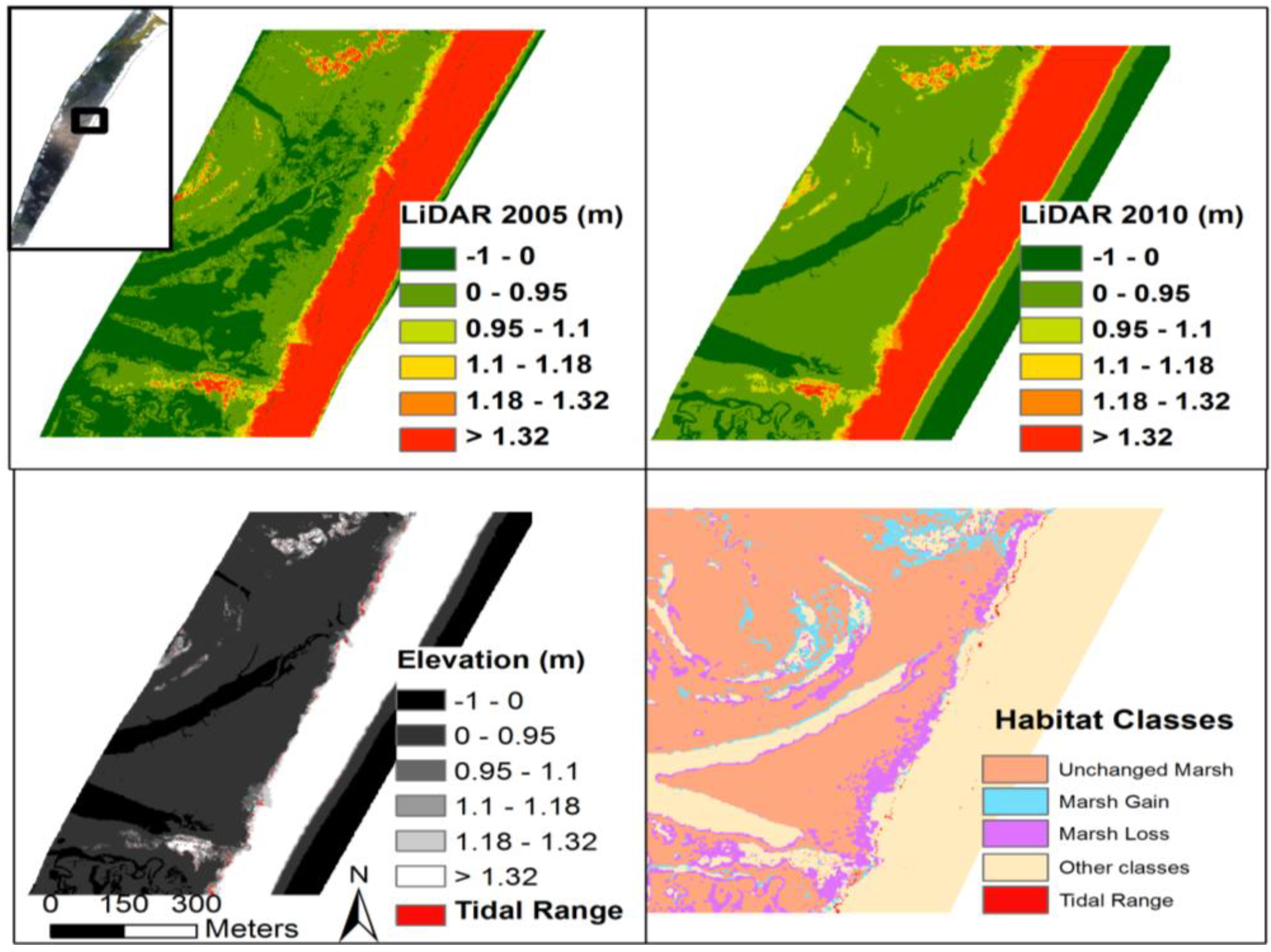
1.6. Light Detection and Ranging (LiDAR) Data

Topography is a key parameter that influences many of the processes involved in coastal change. Therefore, up-to-date high-resolution elevation data are useful for precisely modeling the coastal environment [10]. Airborne laser surveying is a type of remote sensing known as LiDAR, which collects elevation data of land cover surfaces with a high vertical accuracy (i.e., decimeter level). Multiple returns enable the creation of digital elevation models from laser surveys using bare earth elevation and it is possible to reconstruct canopy elevations using first returns. Airborne LiDAR has been useful in mapping coastal terrain because of the ability to rapidly survey long stretches of shorelines [24,25,26]. Brock et al. [16] thoroughly describe the basic principles behind LiDAR coastal topographic surveys conducted by the combined NASA, USGS, and NOAA “lower 48” coastal mapping project.

Using LiDAR data merged with satellite imagery has been shown to increase land cover classification accuracy and reduce errors of omission (percentage of incorrectly classified pixels) [26]. Misclassification is a common problem with multi-spectral satellite imagery, especially between spectrally similar habitats such as water and emergent marsh, so incorporating elevation may be useful for distinguishing between habitats and increasing the classification accuracy. Lee and Shan [25] fused IK multi-spectral with LiDAR elevation data to classify coastal land cover at Camp Lejeune, North Carolina, USA. Supervised and unsupervised classifications were used both on the IK image alone and the LiDAR-fused image. Using typical coastal classes (i.e., marsh, forest, sand), accuracy of the LIDAR-fused imagery was greater than that of the IK image alone. The marsh class omission error decreased by 7% with the LIDAR-fused image, and commission error was 0%, which means that no non-marsh pixels were incorrectly included in the marsh class.

LiDAR can also be used to derive the texture of a ground surface. In remote sensing, texture refers to spatial variation in the brightness of digital images [27]. LiDAR images vary in brightness because smooth surfaces (e.g., sand) tend to reflect more light back to the sensor than rough surfaces (e.g., marsh), which tend to scatter more light. Lu et al.’s [28] study indicated that fusing satellite imagery with texture data can improve classification accuracy.

1.7. Project Significance and Objectives

Remote sensing analysis of barrier island ecosystems using a combination of WV-2, QB, IK, and LiDAR and a variety of classification techniques provides new information that is useful for future coastal habitat mapping. The following hypotheses were tested:

• The new WV-2 sensor will produce more accurate maps in comparison to QB and IK.
• Supervised classification will produce more accurate maps in comparison with unsupervised.
• LiDAR elevation and texture data will increase the map accuracy.

Results from this study will update the NC NERRS Masonboro Island habitat map and provide management officials a plan for future habitat changes by identifying the vulnerable areas of this quickly changing ecosystem [29]. The dominant patterns of habitat change that occur at this coastal area can be applicable and compared to similar barrier islands elsewhere.

Two important components to coastal management today are public outreach and predicting potential impacts due to climate change. While it is certainly important for research results to go directly to policy-makers and management officials, public awareness is necessary for sustaining long-term coastal sustainability and outreach to the public with easily-accessed data and results could be very helpful. Therefore, data and results of this study have been made available via a mapping website (www.uncw.edu\gis) through a map server housed at the University of North Carolina Wilmington.

2. Methodology

The majority of this study involved computing a variety of image classification techniques. Therefore, the methods for this study comprised: (1) gathering satellite imagery and LiDAR data; (2) computing land cover maps; (3) calculating an accuracy assessment; and (4) calculating land cover change.

2.1. Pre-Processing

The three types of imagery, WV-2, QB and IK, had different spatial, spectral, and radiometric characteristics (see Table 1). The IK imagery was ordered as a pan-sharpened, 8-bit image with only visible bands (no near-infrared band). Both WV-2 and QB had multi-spectral bands, as well as a panchromatic band, which enabled these images to be pan-sharpened, and collected reflectance at the higher 11-bit (stored as 16-bit in WV-2) radiometric resolution. The IK image was useful for comparing with the other two higher resolution images. As is the case with many remote sensing projects, a single image rarely covers the entire study area. Therefore, there were two WV-2 images and two IK images to cover the study area. The NERRS Masonboro Island study area was clipped from the imagery.

ENVI offers several methods for pan-sharpening multispectral imagery. The three most popular methods were tested to determine which is the most accurate for this study area: Gram-Schmidt, Color Normalized Spectral Sharpen, and Principal Components. Each pan-sharpened image was then classified and the Principal Components method resulted in the greatest accuracy. For multi-temporal analysis, un-calibrated relative pixel values, or digital numbers, of each spectral band must be corrected for atmospheric effects and converted to spectral reflectance [30]. ENVI’s QUick Atmospheric Correction (QUAC) tool was used to correct all satellite images for atmospheric interference.

The LiDAR data were obtained from the Army Corps of Engineers (ACOE) in LAS format for 2005 (dates collected: 24 and 26 September) and 2010 (date collected: 30 May) at 1 m horizontal spatial resolution and 0.15 m vertical accuracy. Unfortunately, the data did not cover the entire Masonboro NERRS study area; it extended approximately 500 m from the shoreface landward, excluding roughly half of the study area. LiDAR elevation and texture data were fused with the satellite images for subsequent image classification. The output resolution for each layer stack was set to the coarsest spatial resolution of the input data, which means the data were not resampled to a higher spatial resolution than when they were collected.

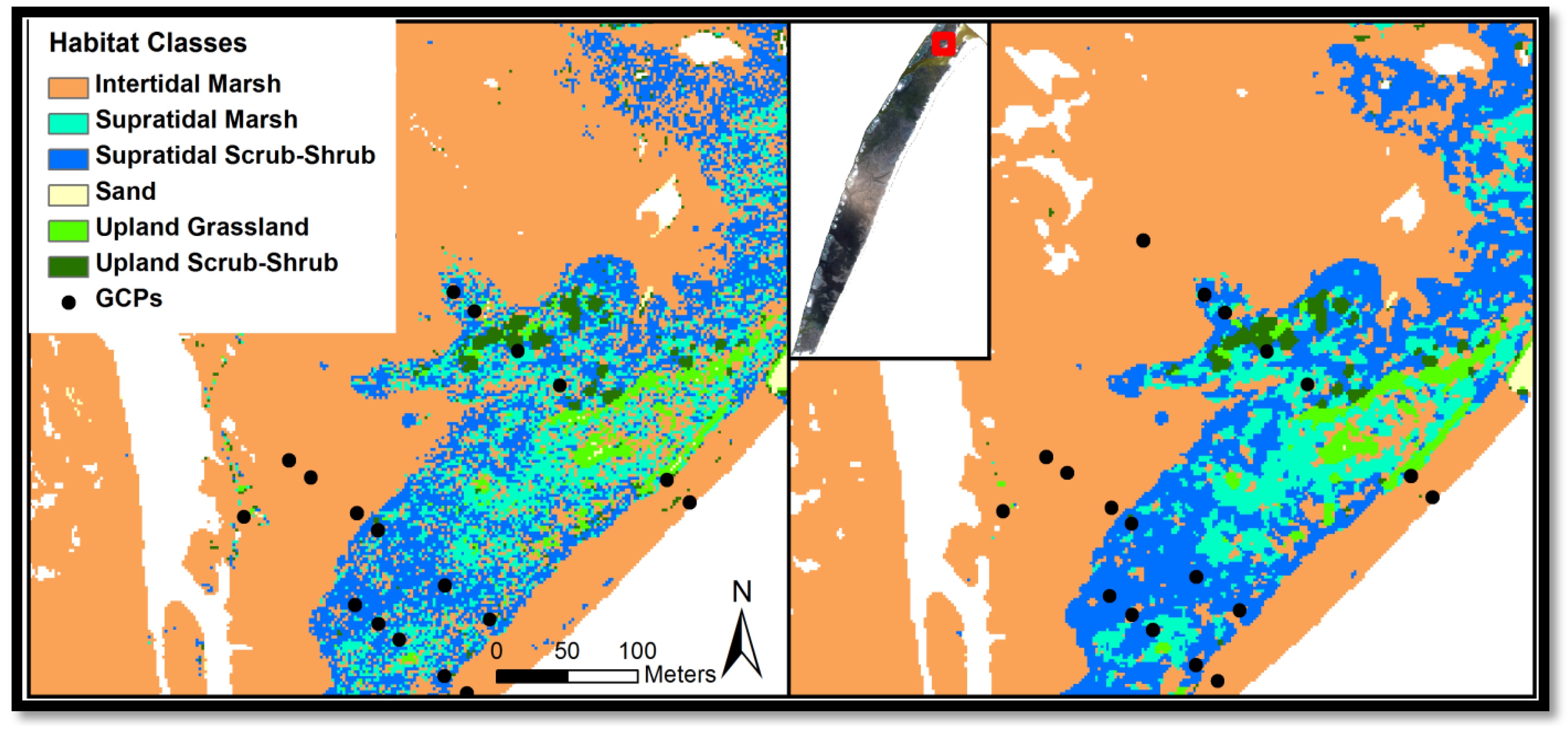
2.2. Habitat Mapping Classification Scheme

The Masonboro NERRS has developed a peer-reviewed habitat classification scheme that has been applied to mapping products, proved useful and effective, and therefore was used for this project [7]. The NERRS recognized, in 2005, the need for a standardized habitat classification scheme, and established a technical workgroup to research, identify, and recommend an existing classification scheme to be used for local, regional, and national site assessment and change analyses. The workgroup found a number of existing methodologies for mapping coastal habitats, but none provided sufficient scope and resolution. Instead of creating a new classification scheme, they decided to build a scheme from the existing U.S. Fish and Wildlife Service’s National Wetland Inventory system [7].

2.3. Satellite Image Classification Techniques

Unsupervised and supervised image classification techniques were performed on the three types of imagery with several combinations of bands, elevation, and texture. Unsupervised classification is a technique that is often used when there is limited or no access to a study area. Therefore, this technique was performed prior to conducting field work in order to minimize any potential bias in the classification results. A mask was first created to exclude open water from each image. Next, ENVI’s ISODATA unsupervised classification tool was performed on each image. The software uses algorithms that group pixels into a specified number of classes based on the natural clusters present in the image and then the image analyst defines the habitat class for each of the spectral classes [31]. For this project, 30 classes were identified during the ISODATA process to account for the 15 classes mapped by NC NERRS in 2004 [4]. Then these images were visually compared with orthophotography from the same year to merge the 30 spectral classes into a final classified image with 8 classes that were identifiable by the analyst based on the NERRS classification scheme. Later these 8 classes were combined into the same 6 classes used in the supervised classification.

Maximum likelihood supervised classifications were performed because this technique has been useful in mapping vegetation [32,33] and is the most widely-used supervised classification method [17]. The technique evaluates the variance and covariance (a measure of the relationship between brightness values in one band versus another band) between training classes and designates a pixel to a class based on the statistical probability of a pixel being a member of a class.

Field work was necessary to collect Ground Reference Points (GRPs) for use in both the supervised image classification and also for conducting the classification accuracy assessment. In order to determine the correct spacing for collecting field sites, a preliminary field-work session was conducted to test locations for spatial autocorrelation. Spatial autocorrelation represents the degree of similarity among observations in a dataset. In land cover studies it is important to account for spatial interactions in GRPs to remove bias in the supervised classifications. In addition, removing spatial autocorrelation means the GRPs used in the accuracy assessment are independent and the assumptions of the classification methods are met. Sampling at distances in which habitats are not autocorrelated removes potential bias in the spatial patterns of similar habitat types.

The field work was conducted using a Real Time Kinematic (RTK) GPS unit (Trimble 5800 receiver with horizontal and vertical accuracies of 10 mm, and 20 mm, respectively) and points were collected along 6 randomly-selected transects spaced 10 m apart and perpendicular from the beach to the back-barrier. Habitat classes were identified at each point for a total of 167 points. These data were tested for spatial autocorrelation using the acf function in R [34] and the results indicated that habitats were not spatially autocorrelated at a sampling distance of 20 m. Therefore, the next stage of field work was designed where each site was at least 20 m away from each other.

Transects were generated perpendicular to the shoreline using the DSAS tool (http://woodshole.er.usgs.gov/project-pages/DSAS/) in ArcMap and each transect was spaced 50 m apart. Thirty-five transects were randomly selected, each transect was divided into line segments with 20 m lengths and these were then converted to points. All points that were located in water, below mean lower low tide, were removed. Field work was conducted from February 2012, through June 2012, where each transect was surveyed, GPS locations were recorded (horizontal and vertical), a photograph was taken, and the habitat class and supplemental notes were recorded (Figure 3). In total, 659 points were collected and 9 of these points were located in water in the 2002 orthophotography so these were removed for the supervised classification analysis (Table 2). The GRPs were randomly divided into two new shapefiles to create a set of training sites and a set of accuracy assessment points. The training site points were then used in ENVI for the supervised maximum likelihood classifications.

Figure 3. Masonboro National Estuarine Research Reserve System study area with ground reference points along 35 randomly selected transects spaced 50 m apart.

Figure 3. Masonboro National Estuarine Research Reserve System study area with ground reference points along 35 randomly selected transects spaced 50 m apart.

Table 2. Habitat Classification Scheme and Number of Ground Reference Points (adapted from [4]).

Name	# Points 2002/2010 (Total: 650/659)	Dominant Species
Intertidal Emergent Wetland	149/150	Spartina alterniflora (smooth cordgrass)
Intertidal Scrub-Shrub Wetland	47/48	Borrichia frutescens (sea ox-eye)
Supratidal Emergent Wetland	40/40	Spartina patens (salt meadow hay); Distichlis spicata (inland saltgrass); Juncus roemarianus (black needle rush)
Supratidal Scrub-Shrub Wetland	63/63	Borrichia frutescens; Spartina patens; Uniola paniculata (sea oats); Distichlis spicata
Upland Grass	132/140	Spartina patens; Uniola paniculata; Distichlis spicata; Panicum spp.
Upland Scrub-Shrub (Mixed)	67/70	Iva frutescens (marsh elder); Baccharis halimfolia (groundsel tree); Ilex vomitoria (yaupon); Myrica cerifera; Quercus laurifolia (laurel oak); Juniperus virginiana (eastern red cedar)
Upland Forest	31/31	Quercus virginiana (live oak); Ilex vomitoria; Myrica cerifera; Quercus laurifolia; Pinus taeda (loblolly pine); Pinus palustris (longleaf pine)
Marine and Estuarine Unconsolidated Bottom and Sand	121/117	N/A

Table 2. Habitat Classification Scheme and Number of Ground Reference Points (adapted from [4]).

Name	# Points 2002/2010 (Total: 650/659)	Dominant Species
Intertidal Emergent Wetland	149/150	Spartina alterniflora (smooth cordgrass)
Intertidal Scrub-Shrub Wetland	47/48	Borrichia frutescens (sea ox-eye)
Supratidal Emergent Wetland	40/40	Spartina patens (salt meadow hay); Distichlis spicata (inland saltgrass); Juncus roemarianus (black needle rush)
Supratidal Scrub-Shrub Wetland	63/63	Borrichia frutescens; Spartina patens; Uniola paniculata (sea oats); Distichlis spicata
Upland Grass	132/140	Spartina patens; Uniola paniculata; Distichlis spicata; Panicum spp.
Upland Scrub-Shrub (Mixed)	67/70	Iva frutescens (marsh elder); Baccharis halimfolia (groundsel tree); Ilex vomitoria (yaupon); Myrica cerifera; Quercus laurifolia (laurel oak); Juniperus virginiana (eastern red cedar)
Upland Forest	31/31	Quercus virginiana (live oak); Ilex vomitoria; Myrica cerifera; Quercus laurifolia; Pinus taeda (loblolly pine); Pinus palustris (longleaf pine)
Marine and Estuarine Unconsolidated Bottom and Sand	121/117	N/A

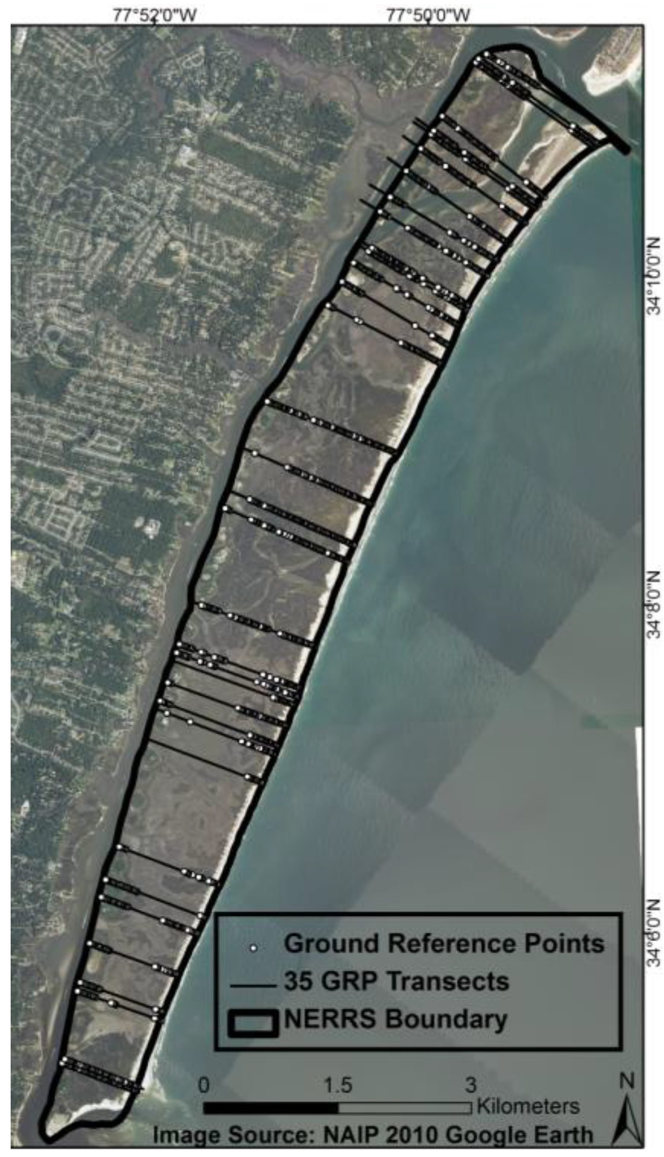
2.4. Accuracy Assessment

Accuracy assessment is compulsory to sound remote sensing classification analysis because it reveals how effectively pixels were grouped into the correct classes by validating them with ground-truth data [35]. Georeferenced GRPs are used with the classification map to generate a confusion matrix that summarizes the number and percentage of points correctly and incorrectly classified for each class, the errors of omission and commission, overall accuracy, and Kappa coefficient. User’s accuracy (also known as commission error) refers to the number or percentage of points included in a class that should not have been. Producer’s accuracy (or omission error) refers to the points that should have been included in a class, but were not. These accuracy statistics are useful in determining how well each class was correctly classified, whereas overall accuracy refers to the percent of pixels correctly classified for the image as a whole. Kappa coefficient considers overall accuracy and individual class accuracy as a means of assessing actual agreement between classification and ground observation, and lies between 0 and 1, where 0 represents agreement due to chance only, and 1 represents complete agreement between the ground truth and the classified image. The Kappa statistic has traditionally been used as a statistically more sophisticated measure of classifier agreement, and may give better inter-class assessment than overall accuracy, but it has also received much controversy as to the true measure of map accuracy [35,36]. It is important to test for accuracy as change detection compares classified images, and, thus, depends on the classification accuracies of individual images [9].

Confusion matrices were generated for each of the classified images. In order to test whether the heterogeneity of the classified images may be influencing the accuracy, a majority 3 × 3 filter was applied to each classified image. This approach replaces isolated cells with the class that corresponds to the majority of cells within a 3 × 3 matrix. Each filtered classified image was then tested for accuracy.

All unsupervised and supervised, all band combinations, and the three types of images were assessed for accuracy. The non-parametric McNemar test was used to compare the classification maps because this technique has been shown to be simple yet robust [36,37]. The McNemar test is similar to the chi squared test where the numbers of incorrectly classified pixels (based on ground reference points) are compared between two classification maps. Research has shown that the McNemar test is a better indicator of map accuracy than the commonly used Kappa statistic [36]. Rozenstein and Karnieli [36] also prefer the McNemar test using this equation:

(1)

where b and c are the off-diagonals, which means these are the number of incorrectly classified pixels in one map versus correctly classified in the other.

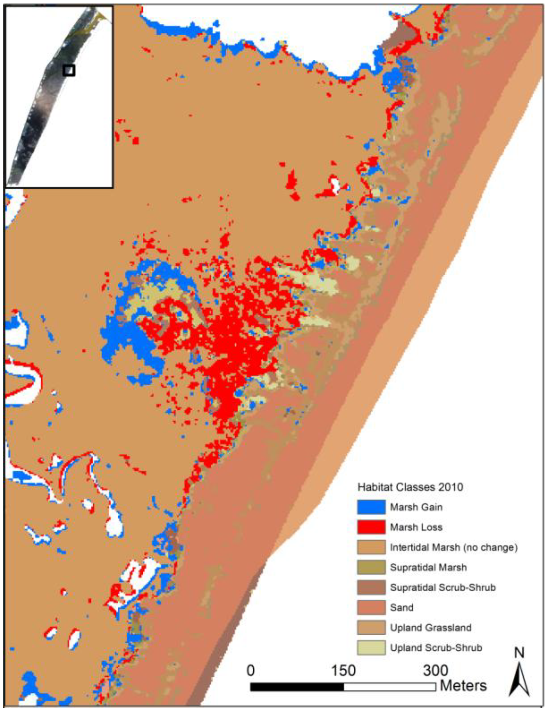
2.5. Habitat Change Detection

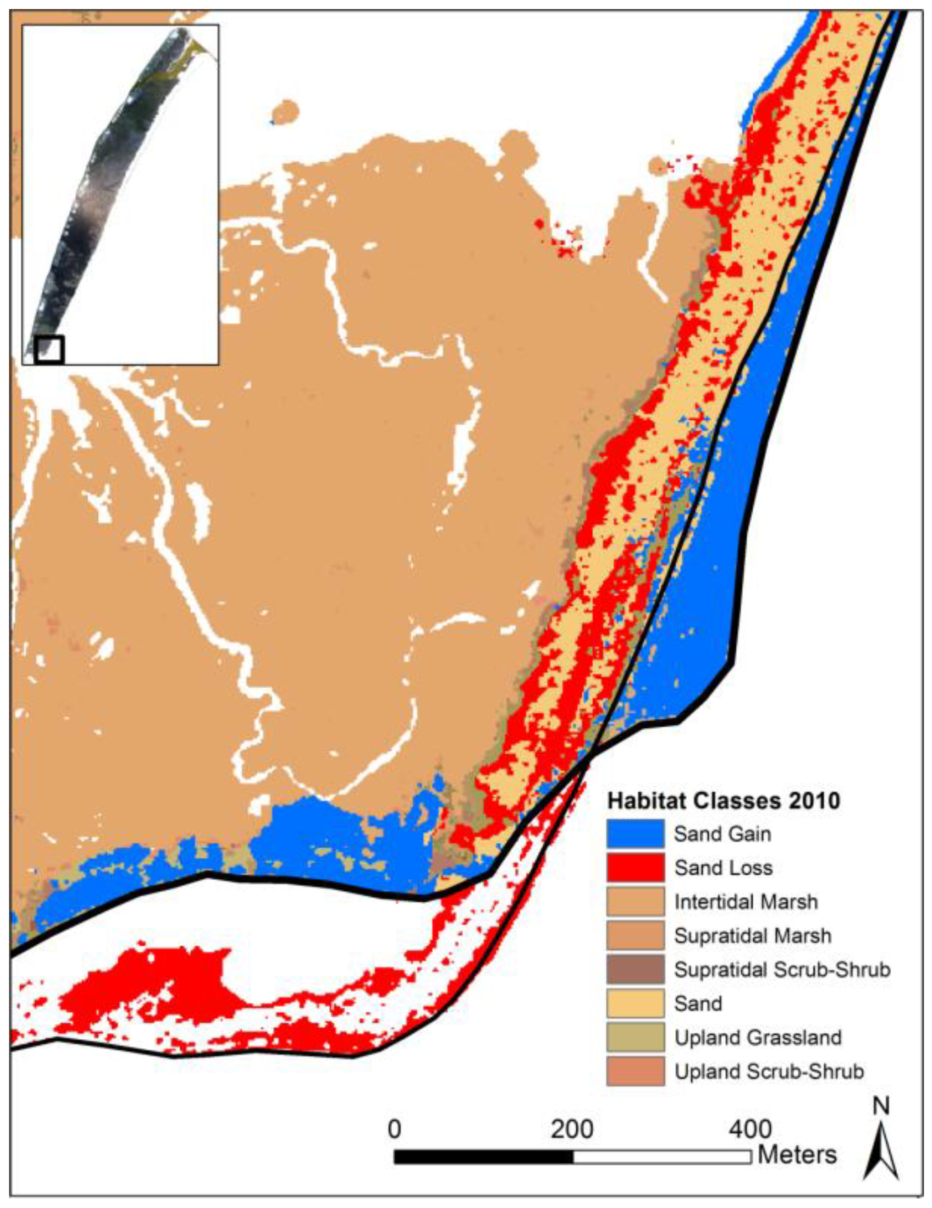
Change detection analysis is useful for identifying where habitat classes have changed through time. Results provide amount and rate of change, spatial distribution of changes, and potentially change trajectories can be calculated [38]. Post-classification change detection compares classified multi-temporal thematic maps, cell by cell. ArcMap tools were used to tabulate change on the best 2002 and 2010 NERRS and Masonboro Island maps. To compare dates, maps were resampled to the coarser map when the two maps were of different spatial resolutions. The conventional method of assessing change using a change detection or classification matrix is widely used, but fails to provide an estimate of the probability that the observed results could have been obtained by chance (i.e., statistical significance). Therefore, Pontius et al. [39] developed methods to extend the classification matrix to changes that are significant, or more than expected.

3. Results

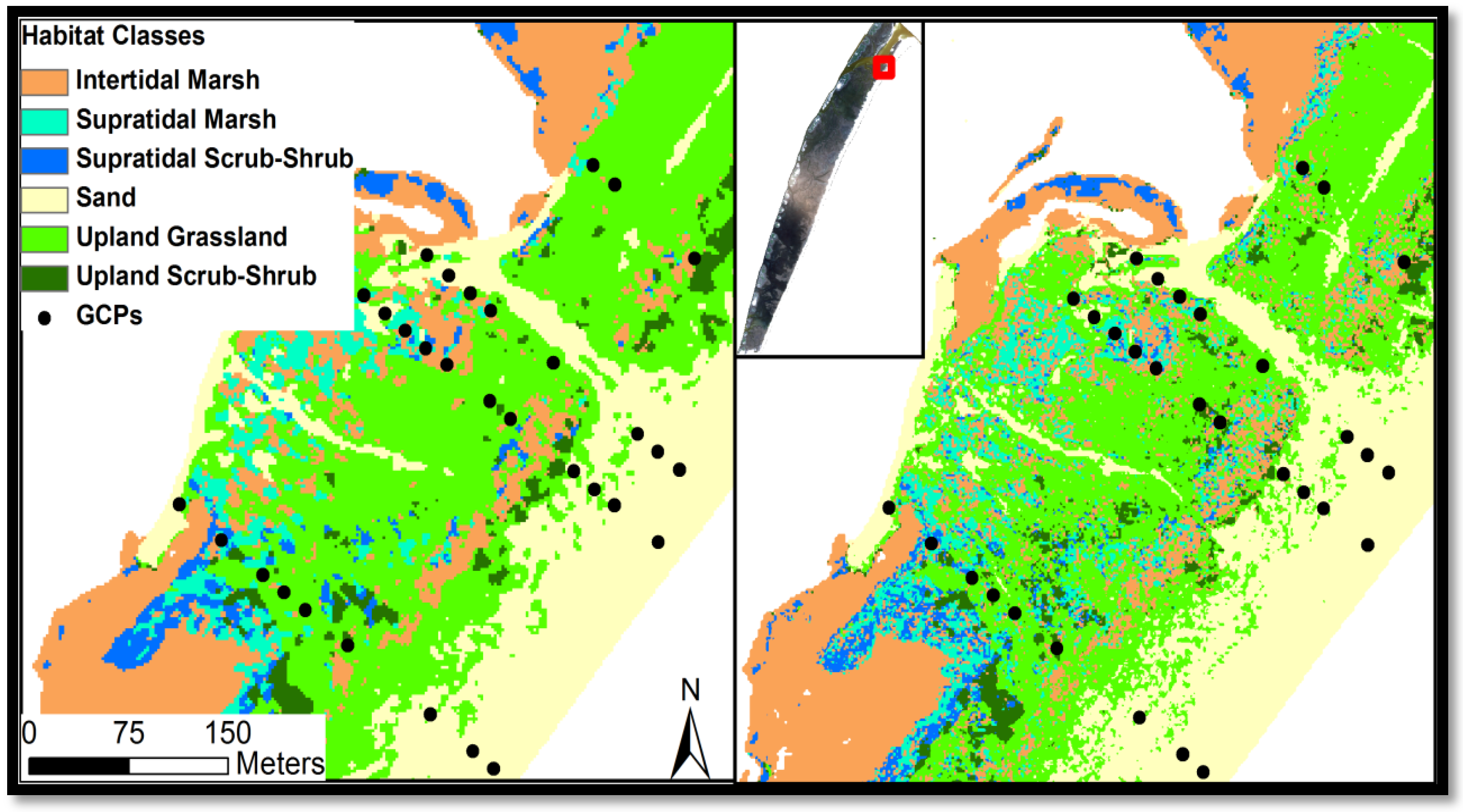
3.1. Masonboro NERRS Study Area

A total of 44 classification maps were generated for the larger NERRS study area and 124 maps were generated for just the Masonboro Island area (including the LiDAR elevation and texture analysis). All maps were assessed for classification accuracy using half the GRPs that were collected for each habitat class. In comparing the WV-2, QB, and IK imagery the most accurate sensor was WV-2, based on overall accuracies and Kappa coefficients (Table 3). IK imagery performed most poorly due to the haze in the imagery, the lowest pan-sharpened spatial resolution, and the lack of a near-infrared band. WV-2’s new spectral bands had mixed results, but generally improved the results. Most supervised classifications were more accurate than the corresponding unsupervised (Figure 4). Pan-sharpening improved map accuracy in only 40% of the maps (Figure 5) while smoothing the classified imagery using a 3 × 3 majority filter improved the classification accuracy in almost all of the maps (77%) (Figure 6).

Table 3. Accuracy assessment (in percent correct) and Kappa coefficients for unsupervised and supervised classifications *.

Sensor	Sharpen	BandCombinations	UNSUPERVISED	Kappa	Majority Filter	Kappa	SUPERVISED	Kappa	Majority Filter	Kappa
WV2 2010	No	NIR, G, B	63.32	0.554	64.71	0.5721	69.21	0.62	71.34	0.646
		All 8	64.01	0.568	64.01	0.5676	66.77	0.59	72.56	0.664
	Pan	NIR, G, B	60.9	0.521	62.28	0.5388	59.15	0.508	60.06	0.52
		All 8	62.63	0.548	64.01	0.566	65.24	0.573	65.85	0.582
	No	Red Edge, yellow, coast	58.48	0.497	59.17	0.5046	70.43	0.635	71.95	0.653
	Pan	Red Edge, yellow, coast	63.67	0.556	63.67	0.5567	59.45	0.511	59.76	0.516
QB 2002	Non	NIR, G, B	57.04	0.485	58.8	0.5028	57.14	0.471	60.25	0.507
		All 4	58.1	0.496	55.99	0.4716	62.11	0.531	61.8	0.527
	Pan	NIR, G, B	57.75	0.487	57.75	0.4862	60.87	0.512	61.8	0.524
		All 4	60.92	0.525	62.32	0.5405	59.63	0.502	60.25	0.51
IK 2002	Pan	R, G, B	40.49	0.257	41.55	0.2679	40.99	0.277	41.3	0.28

* Maps in bold were compared using McNemar tests.

Table 3. Accuracy assessment (in percent correct) and Kappa coefficients for unsupervised and supervised classifications *.

Sensor	Sharpen	BandCombinations	UNSUPERVISED	Kappa	Majority Filter	Kappa	SUPERVISED	Kappa	Majority Filter	Kappa
WV2 2010	No	NIR, G, B	63.32	0.554	64.71	0.5721	69.21	0.62	71.34	0.646
		All 8	64.01	0.568	64.01	0.5676	66.77	0.59	72.56	0.664
	Pan	NIR, G, B	60.9	0.521	62.28	0.5388	59.15	0.508	60.06	0.52
		All 8	62.63	0.548	64.01	0.566	65.24	0.573	65.85	0.582
	No	Red Edge, yellow, coast	58.48	0.497	59.17	0.5046	70.43	0.635	71.95	0.653
	Pan	Red Edge, yellow, coast	63.67	0.556	63.67	0.5567	59.45	0.511	59.76	0.516
QB 2002	Non	NIR, G, B	57.04	0.485	58.8	0.5028	57.14	0.471	60.25	0.507
		All 4	58.1	0.496	55.99	0.4716	62.11	0.531	61.8	0.527
	Pan	NIR, G, B	57.75	0.487	57.75	0.4862	60.87	0.512	61.8	0.524
		All 4	60.92	0.525	62.32	0.5405	59.63	0.502	60.25	0.51
IK 2002	Pan	R, G, B	40.49	0.257	41.55	0.2679	40.99	0.277	41.3	0.28

* Maps in bold were compared using McNemar tests.

Figure 4. Supervised and unsupervised classification maps for an example spoil island. On the left is WV-2 supervised, non-sharpened, 8 bands, majority filtered (72.56% accurate) and on the right is WV-2 unsupervised, non-sharpened, 8 bands, majority filtered (64.01% accurate).

Figure 4. Supervised and unsupervised classification maps for an example spoil island. On the left is WV-2 supervised, non-sharpened, 8 bands, majority filtered (72.56% accurate) and on the right is WV-2 unsupervised, non-sharpened, 8 bands, majority filtered (64.01% accurate).

Figure 5. Pan-sharpened and non-sharpened maps for a portion of the northern beach area. On the left is WV-2 supervised, 8 band, majority filtered, non-sharpened at 1.8 m spatial resolution (72.56% accurate) and on the right is the same image processing with pan-sharpening at 0.5 m spatial resolution (65.85% accurate).

Figure 5. Pan-sharpened and non-sharpened maps for a portion of the northern beach area. On the left is WV-2 supervised, 8 band, majority filtered, non-sharpened at 1.8 m spatial resolution (72.56% accurate) and on the right is the same image processing with pan-sharpening at 0.5 m spatial resolution (65.85% accurate).

Figure 6. Non-filtered and filtered maps with a 3 × 3 majority filter for an example back barrier area. On the left is WV-2 supervised, non-filtered, non-sharpened, 8 band (66.77% accurate) and on the right is the same classification with a majority filter (72.56% accurate).

Figure 6. Non-filtered and filtered maps with a 3 × 3 majority filter for an example back barrier area. On the left is WV-2 supervised, non-filtered, non-sharpened, 8 band (66.77% accurate) and on the right is the same classification with a majority filter (72.56% accurate).

McNemar statistics were computed for each of the highest accuracy classification results in order to determine which maps best represent the study area. For WV-2, the three best classifications (all supervised) were compared, and only one combination showed a significant difference. The highest accuracy map was the WV-2 using all 8 bands (72.56%) but it was not significantly different, (at the 95% level) from the NIR/G/B map (at 71.34%), nor the Red Edge/Yellow/Coastal Blue map (at 71.95%). However, the all-8 map had significantly fewer incorrectly classified GRPs at 25 versus the Red Edge/Yellow/Coastal Blue map at 42 incorrect GRPs and the NIR/G/B at 35 incorrect GRPs. Therefore, the all-8 map was chosen as the best map to represent the 2010 date.

In contrast, all QB map comparisons were significantly different at 95% confidence. Of these, the 4 bands, supervised, non-sharpened, majority filtered map (at 61.8% accurate) had the fewest incorrect GRPs. Therefore, it was chosen as the map that best represented the NERRS study area in 2002.

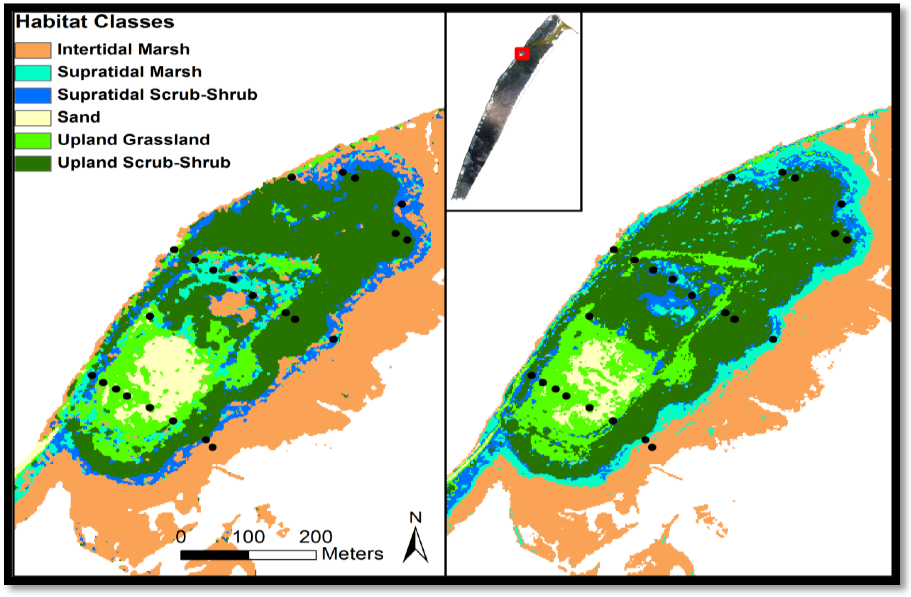
3.2. Masonboro Island Study Area

Given that the LiDAR data was only available for Masonboro Island, these image classifications were assessed using GRPs that were located on the island (Table 4). Similarly to the entire NERRS area, the supervised technique produced more accurate results in comparison to the unsupervised classification maps. The best result was WV-2’s supervised, non-sharpened, majority filtered, 8-band image (80.39%, 0.7417 Kappa). The most accurate sensor for Masonboro Island was WV-2 (Figure 7) and QB had higher accuracy results compared to IK.

Pan-sharpening improved classification accuracy in only 46% of the WV-2 maps and 58% of the QB maps. These results are better in comparison to the entire NERRS study area, which is due to the addition of the LiDAR data. The combination of LiDAR and the new WV-2 spectral bands led to improved results when the images were pan-sharpened. Smoothing the Masonboro Island classifications using a 3 × 3 majority filter also improved overall accuracy. The addition of the LiDAR elevation and texture data sometimes improved the overall classification accuracy, but not in all cases. For example, with WV-2, clearly the better technique was supervised, and the addition of elevation improved the accuracy in 75% of the maps. However, when maps that included elevation data were majority filtered the results are mixed with only half improving with the elevation data. Importantly, the highest accuracy map (at 80.39%) did not use the LiDAR data.

Texture data clearly did not improve the results and in fact had worse results with all maps. Interestingly, the elevation data improved the accuracy with the IK images. Given the overall poor performance of the IK imagery it is small consolation that the elevation data helped the results. Therefore, it is clear from these results that the LiDAR data did not substantially or consistently improve the accuracy of the maps. However, it is worth further investigation since it improved the classification accuracy of the WV-2 imagery.

Table 4. Accuracy assessment (in percent correct) and Kappa coefficients for unsupervised and supervised classifications for the Masonboro Island portion of the NERRS study area.

Sensor	Sharpen	Band Combinations	UNSUPERVISED	Kappa	Majority Filter	Kappa	SUPERVISED	Kappa	Majority Filter	Kappa
WV2 2010	No	NIR, G, B	71.90	0.6263	71.24	0.6188	71.24	0.6206	71.24	0.6196
		All 8	75.16	0.6736	72.55	0.6393	77.12	0.6992	80.39	0.7417
	Pan	NIR, G, B	66.01	0.5439	67.32	0.5616	70.59	0.6185	69.93	0.6104
		All 8	68.63	0.5862	70.59	0.612	71.90	0.6343	73.20	0.6507
	No	Red Edge, yellow, coast	69.28	0.5912	65.36	0.5413	75.16	0.6743	75.82	0.681
	Pan	Red Edge, yellow, coast	69.28	0.5881	69.93	0.5981	70.59	0.6177	71.24	0.6265
	No	NIR, G, Elevation	69.93	0.6017	67.97	0.578	73.20	0.6478	75.16	0.6736
		All 8 + Elevation	66.67	0.5512	67.32	0.5601	68.63	0.57	69.28	0.5758
	Pan	NIR, G, Elevation	69.28	0.5954	67.97	0.5766	72.55	0.6435	70.59	0.5971
		All 8 + Elevation	68.63	0.5855	69.93	0.6017	77.12	0.7026	71.90	0.6142
	No	NIR, G, Texture	67.97	0.5782	67.97	0.5785	68.63	0.5907	72.55	0.6406
		All 8 + Texture	71.90	0.6276	71.24	0.618	70.59	0.599	71.90	0.6162
	Pan	NIR, G, Texture	71.90	0.6293	71.24	0.6208	66.67	56.77	66.67	0.5698
		All 8 + Texture	73.86	0.6540	74.51	0.6623	71.90	0.6178	72.55	0.6242
QB 2002	No	NIR, G, B	60.58	0.4856	60.58	0.4849	60.58	0.4856	68.61	0.5893
		All 4	58.39	0.4551	59.12	0.4649	58.39	0.4551	70.07	0.6074
	Pan	NIR, G, B	59.12	0.4613	59.12	0.4606	59.12	0.4613	70.80	0.6199
		All 4	62.77	0.5103	63.5	0.5187	62.77	0.5103	72.26	0.6389
	No	NIR, G, Elevation	59.85	0.4785	59.12	0.4617	63.50	0.534	65.69	0.5619
		All 4 + Elevation	59.12	0.4620	59.85	0.4688	64.96	0.5559	69.34	0.6074
	Pan	NIR, G, Elevation	60.58	0.4767	59.85	0.4652	61.31	0.5099	66.42	0.5725
		All 4 + Elevation	59.12	0.4618	57.66	0.4425	69.34	0.6057	75.18	0.6764
	No	NIR, G, Texture	59.85	0.4706	59.12	0.4595	60.58	0.4956	60.58	0.4952
		All 4 + Texture	59.12	0.4623	59.85	0.4703	65.69	0.5645	64.96	0.5509
	Pan	NIR, G, Texture	61.31	0.4892	61.31	0.4862	56.93	0.4482	63.50	0.5311
		All 4 + Texture	59.12	0.4607	60.58	0.4795	64.23	0.5378	70.07	0.610
IK 2002	Pan	R, G, B	46.72	0.2801	48.18	0.2995	46.72	0.2801	51.82	0.3798
	Pan	R, G, Elevation	65.38 *	0.5403	67.69 *	0.5678	64.23	0.5339	67.88	0.5833
		All 3 + Elevation	63.08 *	0.5033	65.38 *	0.5315	64.23	0.5345	66.42	0.5657
	Pan	R,G, Texture	62.31 *	0.4924	65.38 *	0.532	49.64	0.3592	52.55	0.397
		All 3 + Texture	63.08 *	0.5050	66.15 *	0.5429	51.09	0.3793	53.28	0.4019

* These images were only able to classify 5 classes (Intertidal Marsh, Supratidal Marsh, Supratidal Scrub-Shrub, Sand, and Upland Grassland). Maps in bold were compared using McNemar tests.

Table 4. Accuracy assessment (in percent correct) and Kappa coefficients for unsupervised and supervised classifications for the Masonboro Island portion of the NERRS study area.

Sensor	Sharpen	Band Combinations	UNSUPERVISED	Kappa	Majority Filter	Kappa	SUPERVISED	Kappa	Majority Filter	Kappa
WV2 2010	No	NIR, G, B	71.90	0.6263	71.24	0.6188	71.24	0.6206	71.24	0.6196
		All 8	75.16	0.6736	72.55	0.6393	77.12	0.6992	80.39	0.7417
	Pan	NIR, G, B	66.01	0.5439	67.32	0.5616	70.59	0.6185	69.93	0.6104
		All 8	68.63	0.5862	70.59	0.612	71.90	0.6343	73.20	0.6507
	No	Red Edge, yellow, coast	69.28	0.5912	65.36	0.5413	75.16	0.6743	75.82	0.681
	Pan	Red Edge, yellow, coast	69.28	0.5881	69.93	0.5981	70.59	0.6177	71.24	0.6265
	No	NIR, G, Elevation	69.93	0.6017	67.97	0.578	73.20	0.6478	75.16	0.6736
		All 8 + Elevation	66.67	0.5512	67.32	0.5601	68.63	0.57	69.28	0.5758
	Pan	NIR, G, Elevation	69.28	0.5954	67.97	0.5766	72.55	0.6435	70.59	0.5971
		All 8 + Elevation	68.63	0.5855	69.93	0.6017	77.12	0.7026	71.90	0.6142
	No	NIR, G, Texture	67.97	0.5782	67.97	0.5785	68.63	0.5907	72.55	0.6406
		All 8 + Texture	71.90	0.6276	71.24	0.618	70.59	0.599	71.90	0.6162
	Pan	NIR, G, Texture	71.90	0.6293	71.24	0.6208	66.67	56.77	66.67	0.5698
		All 8 + Texture	73.86	0.6540	74.51	0.6623	71.90	0.6178	72.55	0.6242
QB 2002	No	NIR, G, B	60.58	0.4856	60.58	0.4849	60.58	0.4856	68.61	0.5893
		All 4	58.39	0.4551	59.12	0.4649	58.39	0.4551	70.07	0.6074
	Pan	NIR, G, B	59.12	0.4613	59.12	0.4606	59.12	0.4613	70.80	0.6199
		All 4	62.77	0.5103	63.5	0.5187	62.77	0.5103	72.26	0.6389
	No	NIR, G, Elevation	59.85	0.4785	59.12	0.4617	63.50	0.534	65.69	0.5619
		All 4 + Elevation	59.12	0.4620	59.85	0.4688	64.96	0.5559	69.34	0.6074
	Pan	NIR, G, Elevation	60.58	0.4767	59.85	0.4652	61.31	0.5099	66.42	0.5725
		All 4 + Elevation	59.12	0.4618	57.66	0.4425	69.34	0.6057	75.18	0.6764
	No	NIR, G, Texture	59.85	0.4706	59.12	0.4595	60.58	0.4956	60.58	0.4952
		All 4 + Texture	59.12	0.4623	59.85	0.4703	65.69	0.5645	64.96	0.5509
	Pan	NIR, G, Texture	61.31	0.4892	61.31	0.4862	56.93	0.4482	63.50	0.5311
		All 4 + Texture	59.12	0.4607	60.58	0.4795	64.23	0.5378	70.07	0.610
IK 2002	Pan	R, G, B	46.72	0.2801	48.18	0.2995	46.72	0.2801	51.82	0.3798
	Pan	R, G, Elevation	65.38 *	0.5403	67.69 *	0.5678	64.23	0.5339	67.88	0.5833
		All 3 + Elevation	63.08 *	0.5033	65.38 *	0.5315	64.23	0.5345	66.42	0.5657
	Pan	R,G, Texture	62.31 *	0.4924	65.38 *	0.532	49.64	0.3592	52.55	0.397
		All 3 + Texture	63.08 *	0.5050	66.15 *	0.5429	51.09	0.3793	53.28	0.4019

* These images were only able to classify 5 classes (Intertidal Marsh, Supratidal Marsh, Supratidal Scrub-Shrub, Sand, and Upland Grassland). Maps in bold were compared using McNemar tests.

McNemar statistics were computed for each of the highest accuracy classification results in order to determine which maps best represent the Masonboro study area from 2010 (WV-2) and 2002 (QB). For WV-2, the most accurate map (supervised, non-sharpened, majority filtered, 8 bands, 80.39%) was compared to the other six maps and none of them were significantly different at the 95% confidence level. Given that there were no significant differences between the best classification maps the highest accuracy map was chosen for the change detection analysis as it also had the fewest incorrectly mapped GRPs.

The most accurate QB map (supervised, 4 bands + elevation, pan-sharpened, majority filtered, at 75.18%) was compared with the four next best maps and again none were significantly different at the 95% confidence level. The most accurate map tied for the fewest incorrect GRPs, and was chosen as the best 2002 map due to its higher overall accuracy.

Figure 7. Supervised classification maps using WorldView-2, QuickBird, and IKONOS for an example area of Masonboro Island.

Figure 7. Supervised classification maps using WorldView-2, QuickBird, and IKONOS for an example area of Masonboro Island.

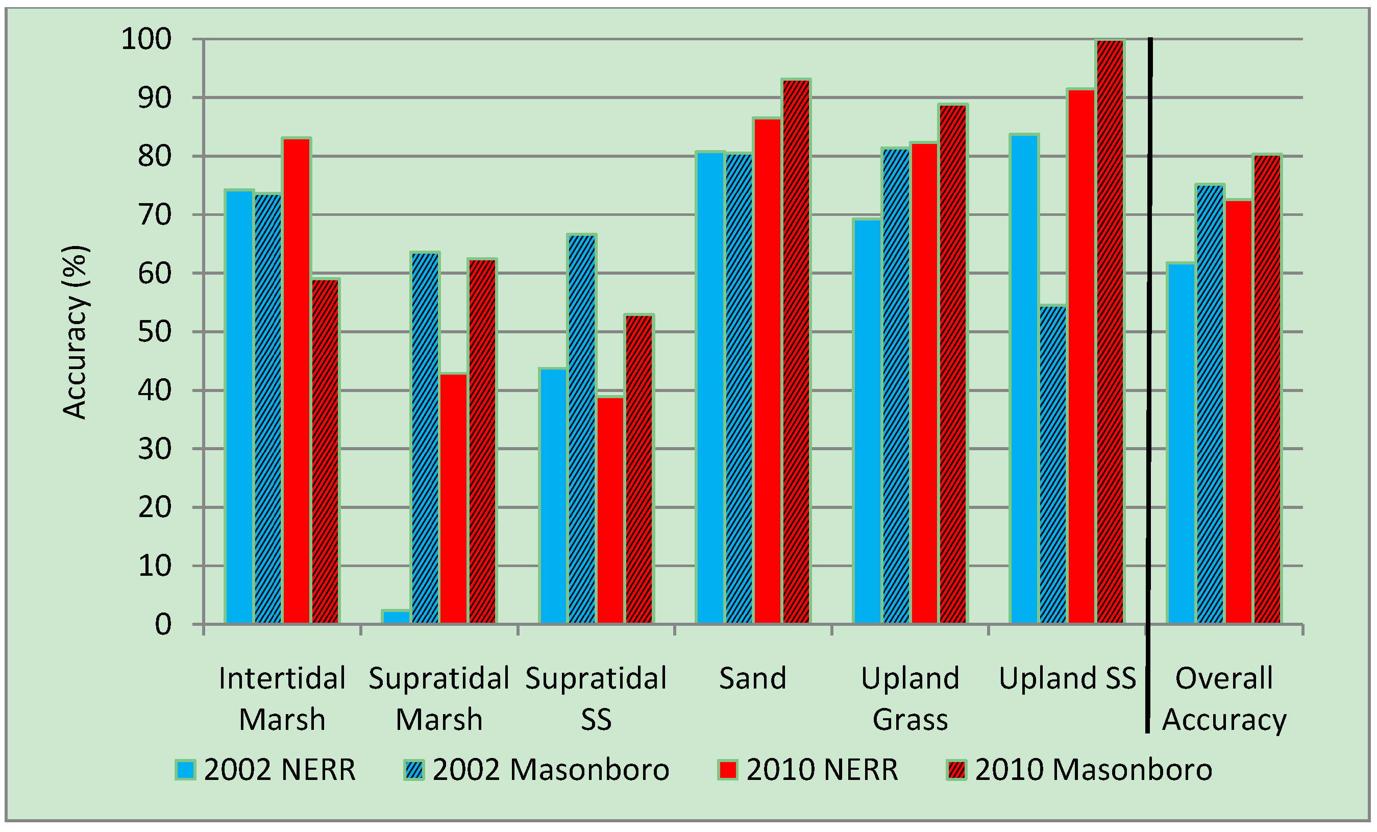
3.3. Habitat Class Accuracies

Accuracy assessment statistics for the best 2002 and 2010 maps reveal that individual class accuracies varied (Figure 8). While the overall map accuracy was lower for the NERRS maps, individual habitat class accuracies varied between the two study areas. For example, the 2010 NERRS intertidal marsh was mapped at 83% accuracy as opposed to only 59% accuracy at Masonboro Island. However, the Masonboro Island map had higher accuracy in every other habitat class. Sand was consistently more than 80% accurate in the best maps. Supratidal marsh and scrub-shrub were poorly classified in the NERRS maps when compared to the Masonboro Island maps. This may be because the back-barrier marsh habitats tended to form in discrete regions adjacent to the water, making them more easily classified than the smaller and more linear marsh habitats surrounding the spoil islands. Emergent wetland grasses tended to be found among the scrub-shrub habitat, and were often taller than the scrub, but not dense enough to dominate the immediate area. It is recommended that NERRS and future analysts use a mixed class for these areas that are a combination of intertidal and supratidal habitats that consist of both grasses and woody scrub to help alleviate this problem. The classification scheme used in this study had no option to designate a “mixed” class.

The higher-resolution (1.8 m) WV-2 NERRS map was more accurate than the QB NERRS map (2.4 m) in all habitat classes except supratidal scrub-shrub. The greatest discrepancy was in the supratidal marsh class, which was misclassified mostly as upland grassland in QB. For Masonboro Island, WV-2 (1.8 m resolution) was more accurate than QB (1 m) in only three habitat classes: sand, upland grassland, and upland scrub-shrub.

Figure 8. Habitat class accuracies for the best maps for 2002 and 2010 for both the NERRS study area and Masonboro Island.

Figure 8. Habitat class accuracies for the best maps for 2002 and 2010 for both the NERRS study area and Masonboro Island.

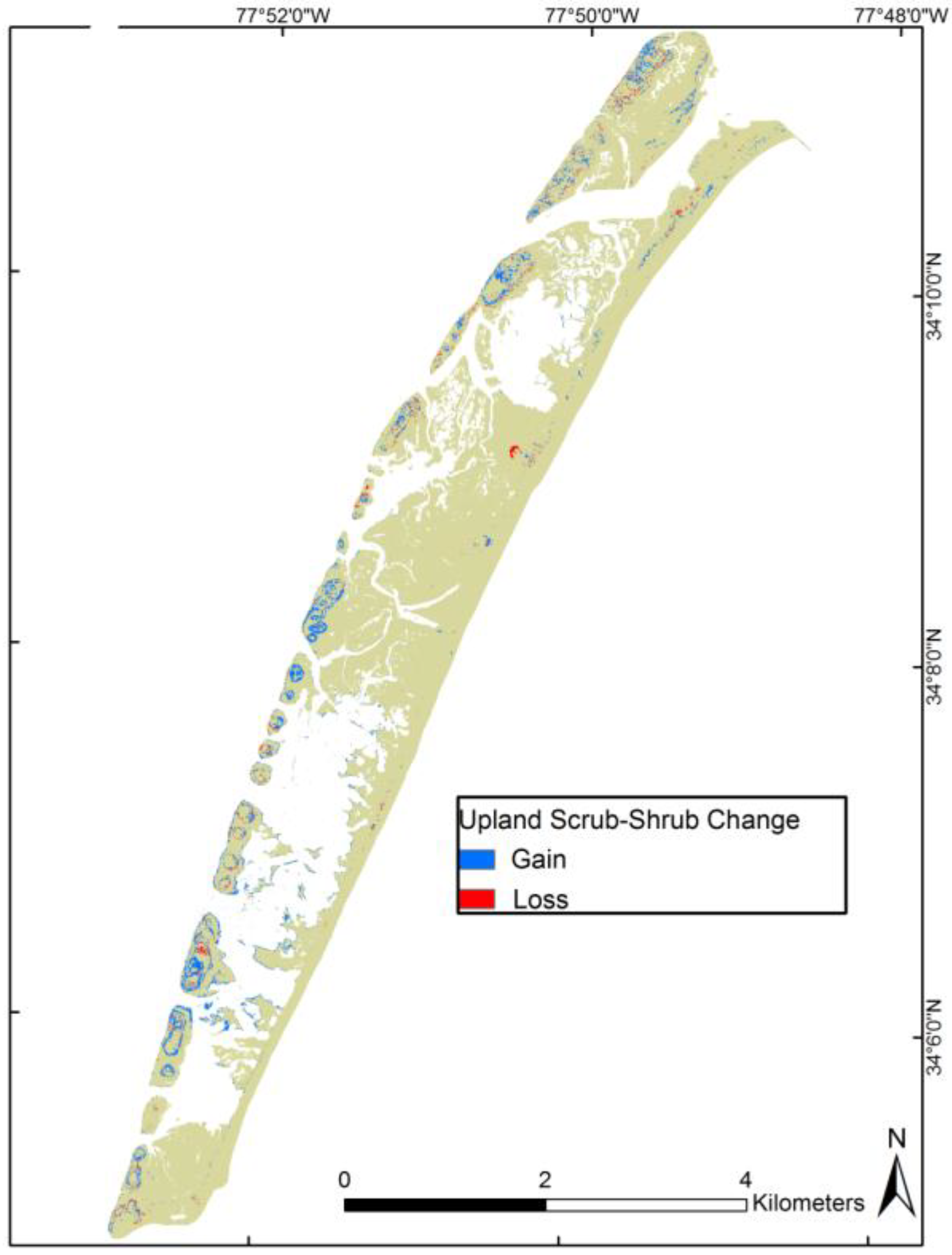
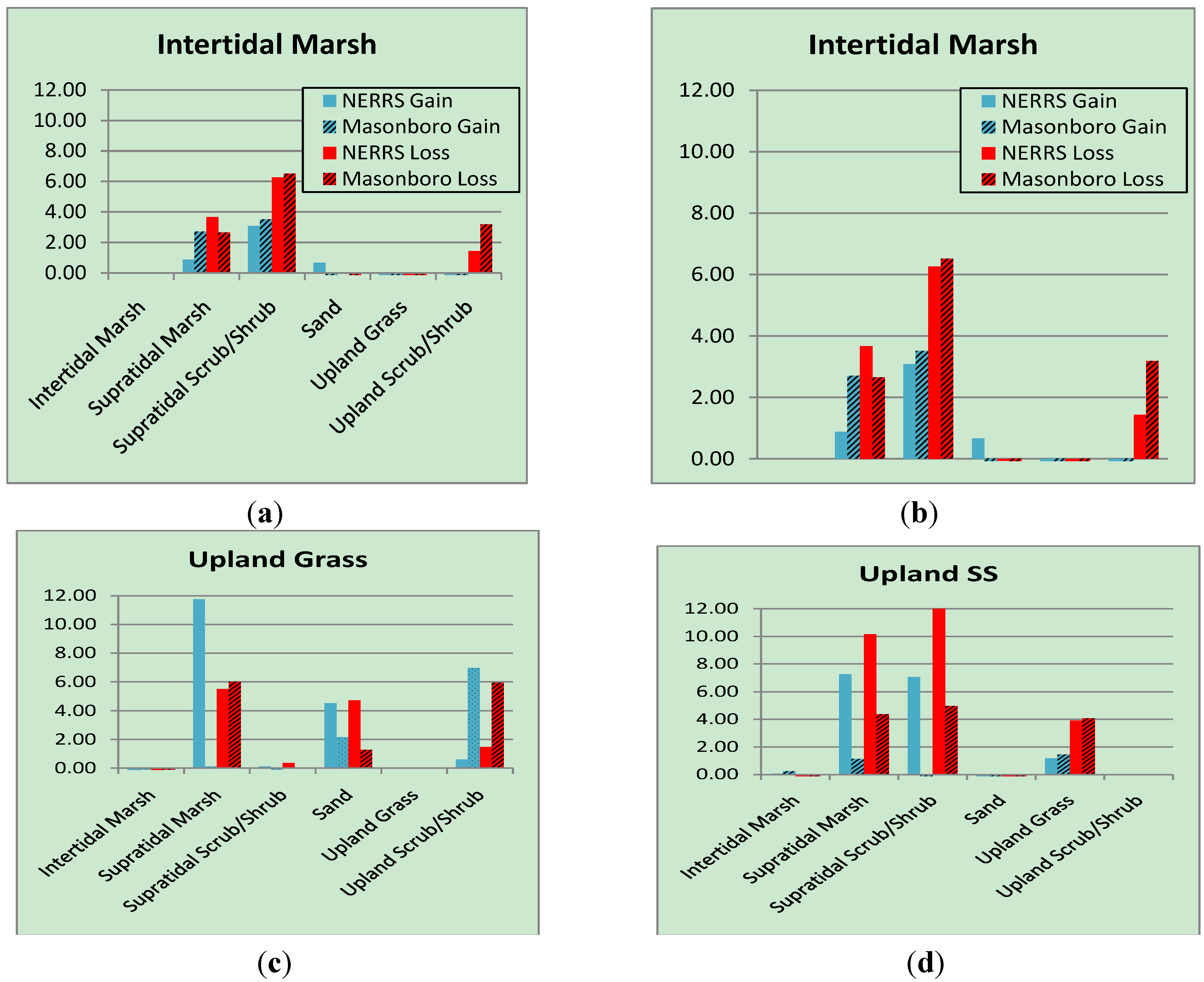
3.4. Habitat Change Analysis

The best classification images for each date (2010 and 2002) and each area (the entire NERRS study area and the Masonboro Island area) were compared using change detection analysis. The higher spatial resolution WV-2 map (1.8 m) was resampled to match the spatial resolution of QB (2.4 m). ArcGIS was used to map the changes and compute change detection statistics from the earlier image (QB 2002) to later (WV-2 2010). Each change matrix displays the change from each class to each other class, as well as how much of each class did not change. Total change is the sum of gains and losses (both numbers are positive), net change is the difference of gains and losses (absolute value of this is only used for study area change, not individual class change).

Change detection results indicate that almost 20% of the NERRS study area experienced changed from 2002 to 2010 (Table 5). Net change (absolute value of the difference of gains and losses) was only 5% of the NERRS, but swap change (difference of total change and net change) accounted for more than 14%. Habitat classes changed in the following order of decreasing total area and total percent change (excluding water): intertidal marsh (2.25 km², 11.50%), sand (1.11 km², 5.70%), upland grassland (0.79 km², 4.02%), supratidal scrub-shrub (0.78 km², 4.01%), supratidal marsh (0.59 km², 3.02%), and upland scrub-shrub (0.57 km², 2.93%) (Table 6).

The most total change, net change and swap change occurred in the intertidal marsh habitat class measured by both individual class area (2.25 km² total, +0.44 km² net, and 1.81 km² swap change) and percent (11.5% total, 2.26% net, and 9.24% swap change) of the NERRS that changed. Intertidal marsh gained most from water (0.71 km²), followed by sand (0.27 km²) and supratidal scrub-shrub (0.21 km²).

With the exception of water, intertidal marsh is the largest habitat class in the study area (6.39 km² in 2010) and changed the most. Sand covered the next largest area (1.21 km² in 2010) and experienced the next most total and net change (1.11 km² or 5.7%, and −0.40 km² or −2.05%, respectively), losing ground mostly to water and intertidal marsh (0.26 km² and 0.21 km², respectively). Upland scrub-shrub increased in area by 84% from 0.57 km² to 0.95 km². Most of this change occurred along the spoil islands, which have been largely inactive as dredge spoil deposition sites during this time period (Figure 9).

Table 5. Percent change of each habitat type across the NERRS study area and at Masonboro Island.

	Gain		Loss		Total Change		Swap		Net (Absolute Value)
	NERRS	Masonboro	NERRS	Masonboro	NERRS	Masonboro	NERRS	Masonboro	NERRS	Masonboro
Intertidal Marsh	6.875	13.243	4.620	4.103	11.495	17.347	9.240	8.206	2.255	9.140
Supratidal Marsh	0.705	0.819	2.314	5.257	3.019	6.076	1.411	1.637	1.608	4.439
Supratidal Scrub/Shrub	2.088	2.378	1.926	6.518	4.014	8.896	3.853	4.756	0.161	4.140
Sand	1.821	5.790	3.874	4.420	5.695	10.211	3.642	8.840	2.053	1.370
Upland Grass	2.328	5.498	1.693	1.903	4.021	7.401	3.386	3.806	0.635	3.595
Upland Scrub/Shrub	2.445	0.974	0.485	1.621	2.929	2.595	0.969	1.948	1.960	0.647
Water	3.342	1.874	4.692	6.754	8.035	8.628	6.685	3.747	1.350	4.881
Total	19.605	30.576	19.605	30.576	19.605	30.576	14.593	16.471	5.012	14.105

Table 5. Percent change of each habitat type across the NERRS study area and at Masonboro Island.

	Gain		Loss		Total Change		Swap		Net (Absolute Value)
	NERRS	Masonboro	NERRS	Masonboro	NERRS	Masonboro	NERRS	Masonboro	NERRS	Masonboro
Intertidal Marsh	6.875	13.243	4.620	4.103	11.495	17.347	9.240	8.206	2.255	9.140
Supratidal Marsh	0.705	0.819	2.314	5.257	3.019	6.076	1.411	1.637	1.608	4.439
Supratidal Scrub/Shrub	2.088	2.378	1.926	6.518	4.014	8.896	3.853	4.756	0.161	4.140
Sand	1.821	5.790	3.874	4.420	5.695	10.211	3.642	8.840	2.053	1.370
Upland Grass	2.328	5.498	1.693	1.903	4.021	7.401	3.386	3.806	0.635	3.595
Upland Scrub/Shrub	2.445	0.974	0.485	1.621	2.929	2.595	0.969	1.948	1.960	0.647
Water	3.342	1.874	4.692	6.754	8.035	8.628	6.685	3.747	1.350	4.881
Total	19.605	30.576	19.605	30.576	19.605	30.576	14.593	16.471	5.012	14.105

Table 6. Percent change in habitats at NERRS from 2002 to 2010.

Area (% of 2002)	Habitat Class in 2010 (Perent)							Class Total (2002)
	Intertidal Marsh	Supratidal Marsh	Supratidal Scrub/Shrub	Sand	Upland Grass	Upland Scrub/Shrub	Water
Intertidal Marsh	25.81	0.33	1.43	0.40	0.19	0.82	1.46	30.43
Supratidal Marsh	0.49	0.31	0.33	0.06	0.81	0.55	0.07	2.63
Supratidal Scrub/Shrub	1.09	0.15	0.77	0.03	0.07	0.55	0.03	2.70
Sand	1.36	0.04	0.02	4.39	1.11	0.04	1.31	8.26
Upland Grass	0.20	0.12	0.07	0.63	2.22	0.21	0.46	3.91
Upland Scrub/Shrub	0.11	0.06	0.19	0.01	0.11	2.44	0.01	2.92
Water	3.63	0.01	0.05	0.68	0.03	0.29	44.46	49.15
Class Total (2010)	32.69	1.02	2.86	6.21	4.54	4.88	47.80	100.00

Table 6. Percent change in habitats at NERRS from 2002 to 2010.

Area (% of 2002)	Habitat Class in 2010 (Perent)							Class Total (2002)
	Intertidal Marsh	Supratidal Marsh	Supratidal Scrub/Shrub	Sand	Upland Grass	Upland Scrub/Shrub	Water
Intertidal Marsh	25.81	0.33	1.43	0.40	0.19	0.82	1.46	30.43
Supratidal Marsh	0.49	0.31	0.33	0.06	0.81	0.55	0.07	2.63
Supratidal Scrub/Shrub	1.09	0.15	0.77	0.03	0.07	0.55	0.03	2.70
Sand	1.36	0.04	0.02	4.39	1.11	0.04	1.31	8.26
Upland Grass	0.20	0.12	0.07	0.63	2.22	0.21	0.46	3.91
Upland Scrub/Shrub	0.11	0.06	0.19	0.01	0.11	2.44	0.01	2.92
Water	3.63	0.01	0.05	0.68	0.03	0.29	44.46	49.15
Class Total (2010)	32.69	1.02	2.86	6.21	4.54	4.88	47.80	100.00

Change detection results focused on the Masonboro Island region of the NERRS show that more than 30% of this area experienced change from 2002 to 2010 (Table 7). To compare the two maps, the pan-sharpened QB map (1.0 m) was resampled to the resolution of the coarser WV-2 map (1.8 m). Of that, more than 16% is attributable to swap change, and 14% due to net change. Habitat classes changed in the following order of decreasing total area and total percent change (excluding water): intertidal marsh (0.99 km², 17.35%), sand (0.58 km², 10.21%), supratidal scrub-shrub (0.51 km², 8.90%), upland grassland (0.42 km², 7.40%), supratidal marsh (0.35 km², 6.08%), and upland scrub-shrub (0.15 km², 2.59%).

Intertidal marsh experienced the most total change and net change (0.99 km² or 17.35%, and 0.52 km² or 9.14%, respectively) with 0.47 km² (8.21%) of swap change (Figure 10). Sand saw the most swap change (0.50 km² or 8.84%), gaining about 0.22 km² from water, while losing about 0.21 km² to upland grassland. Much of the sand gained in 2010 from 2002 water occurred at the southern end of the island along Carolina Beach Inlet where the southeastern tip of Masonboro eroded as much as about 200 meters, and accreted sand along the east-facing beach (Figure 11).

Figure 9. Gain (blue) and loss (red) in upland scrub/shrub for the entire study area *.

Figure 9. Gain (blue) and loss (red) in upland scrub/shrub for the entire study area *.

* Areas in beige are the rest of the study area, and not just persistent scrub-shrub.

Table 7. Percent change in habitats at Masonboro Island from 2002 to 2010.

Area (% of 2002)	Habitat Class in 2010 (Percent)							Class Total (2002)
	Intertidal Marsh	Supratidal Marsh	Supratidal Scrub/Shrub	Sand	Upland Grass	Upland Scrub/Shrub	Water
Intertidal Marsh	25.10	0.29	1.52	0.64	0.23	0.36	1.07	29.21
Supratidal Marsh	3.89	0.36	0.41	0.17	0.37	0.12	0.28	5.62
Supratidal Scrub/Shrub	6.05	0.11	0.65	0.16	0.09	0.05	0.06	7.17
Sand	0.20	0.14	0.02	13.31	3.74	0.03	0.29	17.73
Upland Grass	0.39	0.18	0.07	0.93	5.56	0.19	0.15	7.47
Upland Scrub/Shrub	0.25	0.10	0.30	0.02	0.92	0.32	0.03	1.94
Water	2.45	0.01	0.06	3.87	0.14	0.21	24.11	30.86
Class Total (2010)	38.35	1.18	3.03	19.10	11.06	1.30	25.98	100.00

Table 7. Percent change in habitats at Masonboro Island from 2002 to 2010.

Area (% of 2002)	Habitat Class in 2010 (Percent)							Class Total (2002)
	Intertidal Marsh	Supratidal Marsh	Supratidal Scrub/Shrub	Sand	Upland Grass	Upland Scrub/Shrub	Water
Intertidal Marsh	25.10	0.29	1.52	0.64	0.23	0.36	1.07	29.21
Supratidal Marsh	3.89	0.36	0.41	0.17	0.37	0.12	0.28	5.62
Supratidal Scrub/Shrub	6.05	0.11	0.65	0.16	0.09	0.05	0.06	7.17
Sand	0.20	0.14	0.02	13.31	3.74	0.03	0.29	17.73
Upland Grass	0.39	0.18	0.07	0.93	5.56	0.19	0.15	7.47
Upland Scrub/Shrub	0.25	0.10	0.30	0.02	0.92	0.32	0.03	1.94
Water	2.45	0.01	0.06	3.87	0.14	0.21	24.11	30.86
Class Total (2010)	38.35	1.18	3.03	19.10	11.06	1.30	25.98	100.00

Figure 10. Change in intertidal marsh from 2002 to 2010 at an example back barrier location. Gains in marsh (blue) and losses in marsh (red) tend to occur in close proximity.

Figure 10. Change in intertidal marsh from 2002 to 2010 at an example back barrier location. Gains in marsh (blue) and losses in marsh (red) tend to occur in close proximity.

Figure 11. Change in sand at the southern end of Masonboro Island adjacent to Carolina Beach Inlet. Sand erosion (red) and accretion (blue) can be seen along with overall change from 2002 (thin black line) to 2010 (thick black line).

Figure 11. Change in sand at the southern end of Masonboro Island adjacent to Carolina Beach Inlet. Sand erosion (red) and accretion (blue) can be seen along with overall change from 2002 (thin black line) to 2010 (thick black line).

The change detection results can be further investigated by deriving the difference between observed change and change that would be expected to occur [39]. For gain and loss, expected change was calculated, respectively, as:

(2)

(3)

The analysis is very similar to a chi squared test where the observed and expected are compared. The data are first converted to percentages of change from time 1 to time 2 (e.g., 2002 to 2010) and then the percentage of gain and the percentage of loss are calculated.

Figure 12. The ratio of deviation to expected change for gain (blue) and loss (red) for selected habitat classes. The class in the title gained and lost more than expected over the classes along the x-axis.

Figure 12. The ratio of deviation to expected change for gain (blue) and loss (red) for selected habitat classes. The class in the title gained and lost more than expected over the classes along the x-axis.

Classification change matrices are useful for quantifying change but they do not identify significance of these changes. Therefore, additional computation is required to derive changes that are more or less than expected. The expected percentages of loss and gain are calculated by comparing the observed percentages of each habitat type in time 1 (e.g., 2002). The chi-square statistic is then derived by calculating the difference between observed and expected percentages (termed the deviation), and taking the ratio of this value to the expected percentage. When the ratio of deviation/expectation is greater than 3.84 the gain or loss is significant at the 95% confidence level. These values deviate significantly from expected gain or loss, and are highlighted for the four classes of greatest unexpected change (Figure 12).

Across the study area, there was substantially higher than expected loss than there was gain. For example, with Intertidal Marsh, there was more loss than expected to Supratidal Marsh, Supratidal Scrub-Shrub, and Upland Scrub-Shrub. Conversely, there was almost no significantly greater than expected gain in Intertidal Marsh. Supratidal Marsh and Upland Scrub-Shrub had the largest overall changes and most of the largest gain and loss were from swapping of Supratidal Marsh, Supratidal Scrub-Shrub, and Upland Grass. These results indicate the greater than expected gain and loss from Supratidal Marsh, which is logical considering the fringing location of this habitat type. Upland Grass also had greater than expected change to Supratidal Marsh, Sand and Upland Scrub-Shrub. With sediment accretion around the spoil islands and back barrier of Masonboro (overwash fans) this raises the elevation just enough to expand the Scrub-Shrub habitat and shrink the Supratidal Marsh and Upland Grass. In comparing the losses of all habitat types, it is interesting that the upland classes had more significant loss at Masonboro in comparison to the NERRS as a whole, which experienced significant losses across all habitat types except for upland grassland and intertidal marsh. This suggests that Masonboro Island is more sensitive to erosional forces such as large storm activity.

4. Discussion and Conclusions

It was hypothesized that WV-2 would be the most accurate imagery and it significantly produced more accurate results compared to both QB and IK. The primary factors that distinguished this sensor’s greater map accuracy were a combination of the number of spectral bands, narrow widths of the bands (higher spectral resolution), higher spatial resolution, and greater radiometric resolution. The NIR bands for WV-2, QB and IK cover very similar bandwidths, but the green and especially blue bands are narrower, which may enable WV-2 to more precisely distinguish the vegetation reflectance value. These results confirm the earlier work with QB imagery where the sensor produced map accuracy of only 62% in coastal marsh habitats [20]. The mapping of complex marsh species is problematic with QB due to the lower spectral and spatial resolution. Marsh vegetation is often interspersed with other classes and high spatial resolution is more important in coastal vegetation mapping than high spectral resolution [20]. A study comparing the capabilities of WV-2 and QB sensors to map coastal mangrove species found better spectral separability using WV-2 [40]. A similar study comparing WV-2 and QB land cover classification capabilities found that, in 10 out of 16 classifications, the new WV-2 bands helped achieved higher Kappa values [41]. Spectral un-mixing may be used to assess sub-pixel habitat composition for future studies, but the NERRS classification scheme generally allows for at least 25% of the area, and up to 75%, (i.e., of each pixel) to be mixed with other classes. Two primary reasons for the unsatisfactory classification results with the IK imagery were the lack of a NIR band, and an atmospheric haze that could not be removed from the imagery.

It is important to note that the images were not all acquired at the same calendar dates (see Table 2) and therefore the overall map accuracy and resulting change analysis may be influenced by slightly different phenological periods. This potential issue did not appear to influence image classification or change detection results, but it is recommended that when possible it is best to use images that correspond to the same season. It is also important, when mapping intertidal habitat classes, to acquire images at the same tidal amplitude, make sure to account for tidal datums, and to consider recent precipitation events and how they may affect water levels and standing water on and around the study area. In this study the images were all taken at very close tidal regimes (see Table 2) and did not have any large precipitation event prior to the images being acquired. The tide levels during the capture of images were 1.10 m (QB), and 1.06 m and 1.18 m (both WV-2 images). Given the low relief of the island, however, even a small tidal difference between images could potentially influence habitat mapping. Therefore, the tide elevation and habitat classification was compared using LiDAR data that matched closest with the acquisition dates of the imagery (Figure 13). The LiDAR data had a vertical accuracy of ±0.15 m so the percentage of habitat within the tide levels and accounting for vertical accuracy resulted in a very small percentage of the habitat area mapped. In fact, it is important to remember that the marsh habitats in this study area are emergent, not submerged, and therefore this type of vegetation is mapped at and below sea level given that it extends several meters above the water surface. Given that the habitat type can be mapped when the tide level is well above mean sea level, the tidal regimes were the same given the tolerances for vertical accuracy, and the very small percentage of the area that is located within this elevation, it is concluded that the tidal regime during image acquisition had no effect on the results of the habitat mapping and change detection.

Figure 13. LiDAR elevation data for 2005 (top left) and 2010 (top right) show changes in elevation relative to sea level during this period for a selected area of Masonboro Island. The difference in tidal range (0.08 m; “Tidal Range”) between images used in change detection is overlaid on top of 2010 elevation (bottom left), and on top of the final change detection map (bottom right). This area comprised only 0.36% of the example region, and highlights why tidal differences were considered to not affect the results of the study.

Figure 13. LiDAR elevation data for 2005 (top left) and 2010 (top right) show changes in elevation relative to sea level during this period for a selected area of Masonboro Island. The difference in tidal range (0.08 m; “Tidal Range”) between images used in change detection is overlaid on top of 2010 elevation (bottom left), and on top of the final change detection map (bottom right). This area comprised only 0.36% of the example region, and highlights why tidal differences were considered to not affect the results of the study.

It was hypothesized that the supervised classification technique would provide a more accurate mapping result in comparison to the unsupervised method. Most supervised classifications were more accurate than the corresponding unsupervised. McNemar tests were run on the best maps for each sensor and 10 of 14 (71%) comparisons between supervised and unsupervised maps were significant at the 95% confidence level. Therefore, in this coastal setting and with these sensors the optimal image processing technique was supervised classification. Supervised classification requires in-depth knowledge of the study area, but produces significantly improved classification maps over unsupervised methods. Supratidal marsh and scrub-shrub were poorly classified in the NERRS maps when compared to the Masonboro Island maps. This may be because the back-barrier marsh habitats tended to form in discrete regions adjacent to the water, making them more easily classified than the smaller and more linear marsh habitats surrounding the spoil islands. Emergent wetland grasses tended to be found among the scrub-shrub habitat, and were often taller than the scrub, but not dense enough to dominate the immediate area. It is recommended that NERRS and future analysts use a mixed class for these areas that are a combination of intertidal and supratidal habitats that consist of both grasses and woody scrub to help alleviate this problem. The classification scheme used in this study had no option to designate a “mixed” class.

Future research should combine various methods that identify the optimal image processing technique for each class rather than using only one method, which may identify some classes well while compromising the accuracy of others. By integrating other techniques with the supervised classification technique it is likely that the accuracy can be increased from the highest which is currently just over 80%.

It was hypothesized that LiDAR data (elevation and texture) for Masonboro Island would improve the classification accuracy. The use of LIDAR data for habitat classifications has proved useful in similar projects [42], however, in this study the results were mixed among the three sensors. The LiDAR elevation data substantially improved most of the WV-2 maps and more research should be done with LiDAR data to further evaluate the potential to enhance coastal habitat classification. The texture data had less success compared with elevation but there were some interesting accuracy improvements in some of the techniques so this should be investigated further. One of the reasons the LiDAR may have had limited success is as it was geographically constrained to the Masonboro Island portion of the study area and the range of elevations on Masonboro isn’t as great as the elevation range on the spoil islands.

Change detection results indicate that almost 20% of the NERRS study area and more than 30% of Masonboro Island experienced change from 2002 to 2010. Net change was 5% of the NERRS and 14% of the barrier island, but swap change accounted for more than 14% of the NERRS and 16% of the barrier island total change. This is a substantial amount of change over a relatively short time period. One study found that beach dunes, to which vegetation will soon recruit, can increase in size and extent rapidly—from 13 m² to 3000 m² in 10 years—with interannual fluctuations [42]. Previous research using change detection analysis had net change of less than 7%, but total change from one class to another was greater than 28% [43]. These results are comparable to this study and confirm that it is important when conducting a change analysis to investigate not just the overall change, but class, or swap, changes that can indicate larger changes in the landscape.

The habitat classes that changed most in overall percentage of the study area were intertidal marsh and sand, but these two habitat classes also dominated the study area. They tended to swap with water, indicating erosion, accretion, and perhaps sea level rise. Upland scrub-shrub increased by approximately 84%, mostly along the spoil islands. These spoil islands feature diverse vegetation habitats that have had limited study and should be monitored in the future as scrub and forest continue to develop.

Clearly the Masonboro barrier island habitats change differently than those of the spoil islands. The two primary changes that occurred on the barrier island were erosion of sand and recruitment of vegetation to overwash fans and dunes. The most prevalent changes on the spoil island areas involved marsh changing to other classes. Throughout the entire NERRS, intertidal marsh appears to have gained area mostly in the center of the study area between the upland barrier island and the spoil islands, however, this habitat seems to have lost the most along the spoil islands and back barrier marsh where it existed in close proximity to higher elevation. The intertidal marsh habitat had the most amount of swap change and therefore more research needs to be conducted to isolate the reason for these changes. As others have documented in previous habitat mapping projects, the intertidal marsh habitat is a difficult area to map given the complexity of the water levels, density of plants, and potentially exposed substrate [20].

This study investigated a variety of remote sensing and GIS analytical techniques using new imagery and LiDAR data that can be applied to other coastal areas. Results are directly applicable to coastal management and future habitat mapping projects. It is recommended that WorldView-2 imagery is superior to IKONOS and QuickBird in this coastal setting and if collection of ground reference points is possible it is best to use the supervised method of habitat classification.

References

1. National Oceanic Atmospheric Administration. Barrier Islands: Formation and Evolution. Available online: http://www.csc.noaa.gov/beachnourishment/html/geo/barrier.htm (accessed on 12 April 2011).
2. Sallenger, A.H., Jr. Storm impact scale for barrier islands. J. Coast. Res. 2000, 16, 890–895. [Google Scholar]
3. Andrews, B.D.; Gares, P.A.; Colby, J.D. Techniques for GIS modeling of coastal dunes. Geomorphology 2002, 48, 289–308. [Google Scholar] [CrossRef]
4. Fear, J. A Comprehensive Site Profile for the North Carolina National Estuarine Research Reserve, 2008. Available online: http://www.nerrs.noaa.gov/Doc/PDF/Reserve/NOC_SiteProfile. (accessed on 10 September 2010).
5. Stutz, M.L.; Pilkey, O.H. Open-ocean barrier islands: Global influence of climatic, oceanographic, and depositional settings. J. Coast. Res. 2011, 27, 207–222. [Google Scholar] [CrossRef]
6. Stallings, J.A.; Parker, A.J. The influence of complex systems interactions on barrier island dune vegetation pattern and process. Ann. Assoc. Am. Geogr. 2003, 93, 13–29. [Google Scholar] [CrossRef]
7. Kutcher, T.E. Habitat and Land Cover Classification Scheme for the National Estuarine Research Reserve System, 2008. Available online: http://nerrs.noaa.gov/Doc/PDF/Stewardship/NERRClassificationSchemeDoc.pdf (accessed on 1 May 2011).
8. Sellars, J.D.; Jolls, C.L. Habitat modeling for Amaranthus pumilus: An application of light detection and ranging (LIDAR) data. J. Coast. Res. 2007, 23, 1193–1202. [Google Scholar] [CrossRef]
9. Gratton, C.; Denno, R. Restoration of arthropod assemblages in a Spartina salt marsh following removal of the invasive plant Phragmites australis. Restor. Ecol. 2005, 13, 358–372. [Google Scholar] [CrossRef]
10. Laba, M.; Downs, R.; Smith, S.; Welsh, S.; Neider, C.; White, S.; Richmond, M.; Philpot, W.; Baveye, P. Mapping invasive wetland plants in the Hudson River National Estuarine Research Reserve using Quickbird satellite imagery. Remote Sens. Environ. 2008, 112, 286–300. [Google Scholar] [CrossRef]
11. Pengra, B.; Johnston, C.; Loveland, T. Mapping an invasive plant, Phragmites australis, in coastal wetlands using the EO-1 Hyperion hyperspectral sensor. Remote Sens. Environ. 2007, 108, 74–81. [Google Scholar] [CrossRef]
12. Zhou, H.; Jian, H.; Zhou, G.; Song, X.; Yu, S.; Chang, J.; Liu, S.; Jiang, Z.; Jiang, B. Monitoring the change of urban wetland using high spatial resolution remote sensing data. Int. J. Remote Sens. 2010, 31, 1717–1731. [Google Scholar] [CrossRef]
13. Gesch, D.B. Analysis of LIDAR elevation data for improved identification and delineation of lands vulnerable to sea-level rise. J. Coast. Res. 2009, 53, 49–58. [Google Scholar] [CrossRef]
14. Chust, G.; Galparsoro, I.; Borja, A.; Franco, J.; Uriarte, A. Coastal and estuarine habitat mapping, using LIDAR height and intensity and multi-spectral imagery. Estuar. Coast. Shelf Sci. 2008, 78, 633–643. [Google Scholar] [CrossRef]
15. Zharikov, Y.; Skilleter, G.A.; Loneragan, N.R.; Taranto, T.; Cameron, B.E. Mapping and characterizing subtropical estuarine landscapes using aerial photography and GIS for potential application in wildlife conservation and management. Biol. Conserv. 2005, 125, 87–100. [Google Scholar] [CrossRef]
16. Brock, J.C.; Wright, C.W.; Sallenger, A.H.; Krabill, W.B.; Swift, R.N. Basin and methods of NASA airborne topographic mapper LiDAR surveys for coastal studies. J. Coast. Res. 2002, 18, 1–13. [Google Scholar]
17. Belluco, E.; Camuffo, M.; Ferrari, S.; Modenese, L.; Silvestri, S.; Marani, A.; Marini, M. Mapping salt-marsh vegetation by multispectral and hyperspectral remote sensing. Remote Sens. Environ. 2006, 105, 54–67. [Google Scholar] [CrossRef]
18. DigitalGlobe. The Benefits of the 8 Spectral Bands of WorldView-2. Available online: http://www.digitalglobe.com (accessed on 20 September 2012).
19. DigitalGlobe. QuickBird: Data Sheet. Available online: http//:www.digitalglobe.com (accessed on 20 September 2012).
20. Ghioca-Robrecht, D.M.; Johnston, C.A.; Tulbure, M.G. Assessing the use of multiseason Quickbird imagery for mapping invasive species in a Lake Erie coastal marsh. Wetlands 2008, 28, 1028–1039. [Google Scholar] [CrossRef]
21. Phinn, S.; Roelfsema, C.; Dekker, A.; Brando, V.; Anstee, J. Mapping seagrass species, cover and biomass in shallow waters: An assessment of satellite multi-spectral and airborne hyper-spectral imaging systems in Moreton Bay (Australia). Remote Sens. Environ. 2008, 112, 3413–3425. [Google Scholar] [CrossRef]
22. Wang, Y.; Traber, M.; Milstead, B.; Stevens, S. Terrestrial and submerged aquatic vegetation mapping in fire island national seashore using high spatial resolution remote sensing data. Mar. Geod. 2007, 30, 77–95. [Google Scholar] [CrossRef]
23. Dial, G.; Bowen, H.; Gerlach, F.; Grodecki, J.; Oleszczuk, R. IKONOS satellite, imagery, and products. Remote Sens. Environ. 2003, 88, 23–36. [Google Scholar] [CrossRef]
24. Chust, G.; Grande, M.; Galparsoro, I.; Uriarte, A.; Borja, A. Capabilities of the bathymetric Hawk Eye LIDAR for coastal habitat mapping: A case study within a Basque estuary. Estuar. Coast. Shelf Sci. 2010, 89, 200–213. [Google Scholar] [CrossRef]
25. Lee, S.D.; Shan, J. Combining LIDAR elevation data and IKONOS multispectral imagery for coastal classification mapping. Mar. Geol. 2003, 26, 117–127. [Google Scholar]
26. Woolard, J.W.; Colby, J.D. Spatial characterization, resolution, and volumetric change of coastal dunes using airborne LIDAR: Cape Hatteras, North Carolina. Geomorphology 2002, 48, 269–287. [Google Scholar] [CrossRef]
27. Onojeghuo, A.O.; Blackburn, G.A. Optimising the use of hyperspectral and LIDAR data for mapping reed bed habitats. Remote Sens. Environ. 2011, 115, 2025–2034. [Google Scholar] [CrossRef]
28. Lu, D.; Batistella, M.; Moran, E. Land-cover classification in the Brazilian Amazon with the integration of Landsat ETM+ and Radarsat data. Int. J. Remote Sens. 2007, 28, 5447–5459. [Google Scholar] [CrossRef]
29. Mitasova, H.; Overton, M.F.; Recalde, J.J.; Bernstein, D.J.; Freeman, C.W. Raster-based analysis of coastal terrain dynamics from multitemporal LIDAR data. J. Coast. Res. 2009, 25, 507–514. [Google Scholar]
30. Wu, J.; Wang, D.; Bauer, M.E. Image-based atmospheric correction of QuickBird imagery of Minnesota cropland. Remote Sens. Environ. 2005, 99, 315–325. [Google Scholar]
31. Lillesand, T.; Kiefer, R.; Chipman, J. Remote Sensing and Image Interpretation, 6th ed.; John Wiley & Sons, Inc.: Hoboken, NJ, USA, 2008. [Google Scholar]
32. Chen, S.; Chen, L.; Liu, Q.; Li, X.; Tan, Q. Remote sensing and GIS-based integrated analysis of coastal changes and their environmental impacts in Lingding Bay, Pearl River Estuary, South China. Ocean Coast. Manag. 2004, 48, 65–83. [Google Scholar] [CrossRef]
33. Krause, G.; Bock, M.; Weiers, S.; Braun, G. Mapping land-cover and mangrove structures with remote sensing techniques: A contribution to synoptic GIS in support of coastal management in north Brazil. Environ. Manag. 2004, 34, 429–440. [Google Scholar] [CrossRef]
34. R Core Team. R: A Language and Environment for Statistical Computing; R foundation for statistical computing: Vienna, Austria, 2013. [Google Scholar]
35. Ismail, M.H.; Jusoff, K. Satellite data classification accuracy assessment based from reference dataset. Int. J. Comput. Inf. Sci. Eng. 2008, 2, 96–102. [Google Scholar]
36. Leeuw, J.D.; Jia, H.; Yang, L.; Liu, X.; Schmidt, K.; Skidmore, A.K. Comparing accuracy assessments to infer superiority of image classification methods. Int. J. Remote Sens. 2006, 27, 223–232. [Google Scholar] [CrossRef]
37. Rozenstein, O.; Karnieli, A. Comparison of methods for land-use classification incorporating remote sensing and GIS inputs. Appl. Geogr. 2011, 31, 533–544. [Google Scholar] [CrossRef]
38. Lu, D.; Mausel, P.; Brondizio, E.; Moran, E. Change detection techniques. Int. J. Remote Sens. 2003, 25, 2365–2407. [Google Scholar]
39. Pontius, R.G.; Shusas, E.; McEachern, M. Detecting important categorical land changes while accounting for persistence. Agric. Ecosyst. Environ. 2004, 101, 251–268. [Google Scholar] [CrossRef]
40. Heumann, B. An object-based classification of mangroves using a hybrid decision tree-support vector machine approach. Remote Sens. 2011, 3, 2440–2460. [Google Scholar] [CrossRef]
41. Novack, T.; Esch, T.; Kux, H.; Stilla, U. Machine learning comparison between worldview-2 and quickbird-2-simulated imagery regarding object-based urban land cover classification. Remote Sens. 2011, 3, 2263–2282. [Google Scholar] [CrossRef]
42. Montreuil, A.; Bullard, J.; Chandler, J.; Millet, J. Decadal and seasonal development of embryo dunes on an accreting macrotidal beach: North Lincolnshire, UK. Earth Surf. Processes Landf. 2013, 38, 1851–1868. [Google Scholar] [CrossRef]
43. Manandhar, R.; Odeh, I.O.A.; Pontius, G.R. Analysis of twenty years of categorical land transitions in the Lower Hunter of New South Wales, Australia. Agric. Ecosyst. Environ. 2010, 135, 336–346. [Google Scholar] [CrossRef]