Article

Evaluation of Model Validation Techniques in Land Cover Dynamics

1
School of Geography & Environmental Science, Building 11, Clayton Campus, Monash University, Melbourne, Victoria 3800, Australia
2
Department of Geography & Environmental Studies, University of Rajshahi, Rajshahi 6205, Bangladesh
*
Author to whom correspondence should be addressed.
ISPRS Int. J. Geo-Inf. 2013, 2(3), 577-597; https://doi.org/10.3390/ijgi2030577
Submission received: 30 April 2013 / Revised: 17 June 2013 / Accepted: 19 June 2013 / Published: 26 June 2013

Abstract

:
This paper applies different methods of map comparison to quantify the characteristics of three different land change models. The land change models used for simulation are termed as “Stochastic Markov (St_Markov)”, “Cellular Automata Markov (CA_Markov)” and “Multi Layer Perceptron Markov (MLP_Markov)” models. Various model validation techniques such as per category method, kappa statistics, components of agreement and disagreement, three map comparison and fuzzy methods have then been applied. A comparative analysis of the validation techniques has also been discussed. In all cases, it is found that “MLP_Markov” gives the best results among the three modeling techniques. Fuzzy set theory is the method that seems best able to distinguish areas of minor spatial errors from major spatial errors. Based on the outcome of this paper, it is recommended that scientists should try to use the Kappa, three map comparison and fuzzy methods for model validation. This paper facilitates communication among land change modelers, because it illustrates the range of results for a variety of model validation techniques and articulates priorities for future research.

Graphical Abstract

1. Introduction

A typical approach to land-use and land-cover change (LUCC) modeling is to investigate how different variables relate to historic land transitions, and to then use those relationships to build models to project future land transitions [1,2]. Moreover, in general the spatially-explicit models of LUCC begin with a digital map of an initial time and then simulate transitions in order to produce a prediction map for a subsequent time [3]. Upon seeing the prediction results, questions may arise about the accuracy of the base maps, the performance of the model and whether this predicted map represents the real scenario [4]. In this regard, it is necessary to quantify the map errors, the amount of differences among the maps and to validate the models used for prediction.
With the growth of high-resolution spatial modeling, geographic information systems (GIS) and remote sensing the need for map comparison methods increases. Good comparison methods are needed to perform calibration and validation of spatial results in a structured manner [5]. The importance of map comparison methods is recognized and has growing interest among researchers [6,7]. In general maps are compared for a number of reasons: (1) to compare maps generated by models under different scenarios and assumptions, (2) to detect temporal/spatial changes, (3) to calibrate/validate land-use models, (4) to perform uncertainty and sensitivity analyses and (5) to assess map accuracy. In fact, map comparison may be seen as finding a goodness-of-fit measure [8].
There has been tremendous interest in validation of simulation models that predict changes over time [9,10]. However, there is usually less than perfect agreement between the change predicted by the model and the change observed in the reference maps, which is no surprise, since scientists usually do not anticipate that a model’s prediction will be perfect. Furthermore, scientists rarely believe that the data are perfect. Therefore, a natural question is, “What accounts for the most important disagreements between the prediction and the data: (1) error in the prediction map, or (2) error in the reference maps?” [11]. If precise information on accuracy and error structure is available, then there could be a method to incorporate information concerning data quality into measures of model validation [12,13].
Assessing model performance is a continuous challenge for modelers of landscape dynamics. A common approach is historical validation where a predicted map is compared to an actual map [14]. However, many types of land-use models simulate land-use changes starting from an original land-use map, such as Markov models, cellular automata, logistic regression models, neural networks, etc. Since most locations do no change their land use over the length of a typical simulation period, the similarity between the simulated land-use map and the actual land-use map will be high for most calibrated models [15]. Therefore, to rigorously assess the accuracy of the simulated land-use map, a meaningful reference level is required [16].
The evaluation of spatial similarities and land use change between two raster maps is traditionally based on pixel-by-pixel comparison techniques. This kind of change detection procedure is called the post-classification comparisons [17]. A problem with this traditional approach is that, because they are based on a pixel-by-pixel comparison, they do not necessarily capture the qualitative similarities between the two maps. This problem becomes important when map comparisons (e.g., of actual and predicted land use) are used to evaluate the output of predictive spatial models such as cellular automata based land use models [18]. The lack of appropriate comparison techniques, specially, the ones that can handle qualitative comparisons of complex land use maps for the purpose of evaluating model output, is currently a major problem in the area of predictive simulation modeling [19].
Recently, numerous map comparison methods have been proposed that take into account the spatial relation between cells, as opposed to simple cell-by-cell overlap [20]. These new methods consider, for example, proximity [21], the presence of recognizable structures, i.e., features [22], moving windows [23] or wavelet decomposition [24]. Others have evaluated model performance based on metrics summarizing the whole landscape [25,26].
This is how different methods have been introduced and new software packages are being developed, for the sake of map comparison/validation of models that predict LUCC change from a map of initial time to a map of a subsequent time [2]. This paper addresses these issues and illustrates some methods through a case study from Khulna, Bangladesh to validate the predicted maps. The main objective of this paper is to find out whether the simulation is giving any abrupt result or not and to compare among the different model validation techniques. Therefore, in this paper, we will discuss the advantages and disadvantages of some commonly-used map comparison techniques to assess the agreement between the simulated maps and the actual land-cover maps.
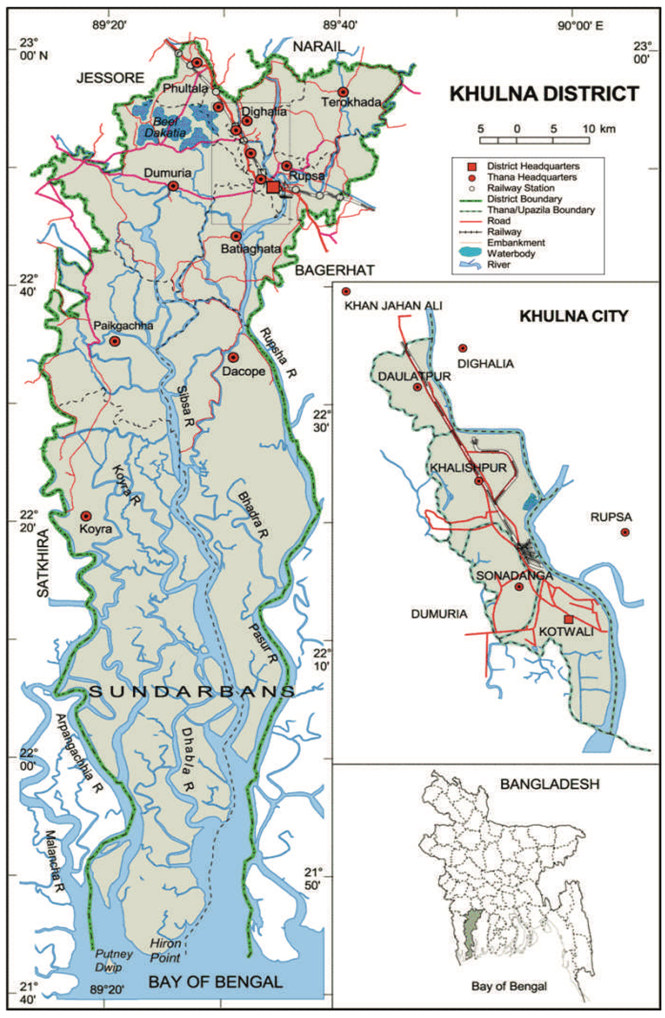
Figure 1. Location of Khulna City in Bangladesh. Source: Banglapedia, National Encyclopedia of Bangladesh, 2012.
Ijgi 02 00577 g001

2. Materials and Methods

2.1. Study Area

The proposed study area is Khulna City Corporation (KCC) and its surrounding impact areas (Figure 1, Figure 2). Geographically, Khulna lies at 22°49'N and 89°34'E. Its mean elevation is seven feet above Mean Sea Level. Khulna is a linear shaped city [27].
Figure 2. Location of the study area (areas of Khulna City Corporation (KCC) and adjoining fringe areas) on Landsat satellite images. (Image source: US Geological Survey (USGS), 2012 and Shapefile source: Khulna City Corporation, 2012).
Ijgi 02 00577 g002
Within the KCC core area, there are roughly 11,280 acres of land. Nearly 10% of this land is not yet in urban use. It means that about 1,100 acres of land are available within KCC for future urban growth [27].

2.2. Remote Sensing Data

To prepare the base maps, the Landsat satellite images (1989, 1999 and 2009) have been collected from the official website of US Geological Survey (USGS). Landsat Path 137 and Row 44 cover the whole study area. The map projection of the satellite images is set as the Universal Transverse Mercator (UTM) within Zone 46 N– Datum World Geodetic System (WGS) 1984. The pixel size of the images is 30 × 30 m.
The following five land cover types have been identified for this research (Table 1) [28]:
Table 1. Land cover types.
Land Cover TypeDescription
Built-up AreaAll residential, commercial and industrial areas, villages, settlements and transportation infrastructure.
Water BodyRiver, sea, permanent open water, lakes, ponds, canals and reservoirs.
VegetationTrees, shrub lands and semi natural vegetation: deciduous, coniferous, and mixed forest, palms, orchard, herbs, climbers, gardens, inner-city recreational areas, parks and playgrounds, grassland and vegetable lands.
Low LandPermanent and seasonal wetlands, low-lying areas, marshy land, rills and gully, swamps, mudflats, all cultivated areas including urban agriculture; crop fields and rice-paddies.
Fallow LandFallow land, earth and sand land in-fillings, construction sites, developed land, excavation sites, solid waste landfills, open space, bare soils.

2.3. Base Map Preparation

A supervised classification method using “Fisher hard classifier” has been applied to prepare the base maps. Fisher classifier performs well when there are very few areas of unknown classes [28]. This is why fisher classifier is selected. Then a mode filter is applied to generalize the fisher classified land cover images. This kind of filtering helps minimizing the isolated pixels. Later the generalized images are reclassified to produce the final version of land cover maps of three different years (Figure 3). The combination is adopted for generating the best possible classification results in this particular context.
After performing change detection analysis, it is found that “builtup area” is increasing while “water body”, “low land” and “fallow land” cover types are decreasing gradually (Figure 4). This is the general trend of land cover change that will be used for simulating the future scenario.

2.4. Accuracy Assessment

The next stage of image classification process is accuracy assessment. It is not typical to ground truth in every pixel of the classified image. Therefore, at first, some reference pixels are generated. A total of 250 reference pixels are generated for each classification image to perform accuracy assessment. The detailed historical base maps (1988, 1999 and 2008) of KCC area are collected from “Survey of Bangladesh” for performing the accuracy assessment. The collected base maps have then been used to find the land cover types of the reference points.
Figure 3. Landcover maps of the study area.
Ijgi 02 00577 g003
Figure 4. Percentages of presence of land cover types (1989–2009).
Ijgi 02 00577 g004
It is known that user’s accuracy for category K is the percent of category K in the reference information, given that the map shows category K. Producer’s accuracy for category K is the percent of category K in the map, given that the reference information shows category K [28]. The overall accuracy represents the percentage of correctly classified pixels [29]. At the end, the producer’s and user’s accuracy for all the years are found ranging approximately from 76% to 95%. While the overall accuracies for 1989, 1999 and 2009 are found 84.20%, 88.80% and 93.60% respectively.

2.5. Simulating Land Cover Maps

In the next stage three different models, using IDRISI Selva® software, are implemented to simulate the land cover maps of Khulna of 2009 [28]. For this purpose, the base maps of 1989 and 1999 are used in all three cases. The first model that has been implemented is given the name as “Stochastic Markov Model (St_Markov)” [30], because this model combines both the Stochastic processes as well Markov Chain analysis techniques [31,32].
Figure 5. Simulated land cover maps of Khulna City (2009).
Ijgi 02 00577 g005
The second model is termed as “Cellular Automata Markov Model (CA_Markov)” [30]. CA_Markov combines the concepts of Markov Chain [32], Cellular Automata [33], Multi-Criteria Evaluation [34] and Multi-Objective Land Allocation [30]. The third model is named as “Multi Layer Perceptron Markov Model (MLP_Markov)” [28]. MLP_Markov combines the concepts of Markov Chain [32], Artificial Neural Network [35] and the Feed-Forward concept of Multi Layer Perceptron Neural Network [36]. The “St_Markov”, “CA_Markov” and “MLP_Markov” methods have been adopted from Ahmed and Ahmed (2012) [28]. The simulated land cover maps are shown in Figure 5.

3. Results and Discussion

Traditionally model validation refers to comparing the simulated and reference maps [37]. Sometimes the simulated maps can give misleading results. In that case, it is necessary to validate the projected/simulated map with the base/reference map. In this section, the comparisons between the actual base map (2009) and the simulated maps (St_Markov, CA_Markov and MLP_Markov) of year 2009 have been performed. The main objective of model validation is to find out whether the simulation is giving any abrupt result or not. This justifies the modeling output in terms of reality.
For validating the simulated maps, two different approaches are adopted. The first one is pixel-based visual approach. This approach helps to reveal the spatial patterns in a quick look. The visual approach is subjective. Another one is statistical approach. This approach is important because it explains the scenario in a quantitative way. There is a general trend in choosing the wrong technique for the purpose of model validation in remote sensing and GIS analysis. This article will help the researchers in selecting the proper model validation technique.

3.1. Per Category Method

The per category comparison method performs a cell-by-cell comparison with respect to one (user selected) category. It simultaneously gives the user information about the occurrence of the selected category in both maps [37]. Figure 6, Figure 7, Figure 8 show the method that performs cell-by-cell comparison for each land cover category. The outputs are depicted in four different legends indication different states of comparison. The more there will be the amount of “both maps”, the better the simulation result.
This is how all the possible combinations (Base Map 2009 vs. St_Markov 2009, Base Map 2009 vs. CA_Markov 2009 and Base Map 2009 vs. MLP_Markov 2009) are taken into consideration. It is then found that the simulated map of “MLP_Markov 2009” shows the best results for all the land cover categories in terms of the highest amount of the legend “in both maps” (Figure 8). This kind of pixel-based per category map comparison method is calculated based on the “Contingency Table”, which details the cross-distribution of categories on the two maps. The table is expressed in number of cells (Table 2, Table 3, Table 4). Three statistics are compared in each confusion matrix: overall accuracy, producer’s accuracy, and user’s accuracy. But this kind of map comparison method cannot perform and formulate the concepts of “error due to quantity” and “error due to location”, in order to partition the total error when comparing maps that show the same categorical variable [38,39].
Figure 6. Per category comparison method (Base Map (2009) vs. St_Markov (2009)).
Ijgi 02 00577 g006
Figure 7. Per category comparison method (Base Map (2009) vs. CA_Markov (2009)).
Ijgi 02 00577 g007
Figure 8. Per category comparison method (Base Map (2009) vs. MLP_Markov (2009)).
Ijgi 02 00577 g008
Table 2. Per category map comparison (Map 1 = Base Map (2009) and Map 2 = St_Markov (2009)).
Land Cover TypeIn both MapsIn none of the MapsOnly in Map 1Only in Map 2
Builtup Area60,574386,747154,00586,098
Water Body12,799655,9638,24010,422
Vegetation87,432497,67143,09159,230
Low Land103,479336,88698,116148,943
Fallow Land60,265509,55459,42358,182
Table 3. Per category map comparison (Map 1 = Base Map (2009) and Map 2 = CA_Markov (2009)).
Land Cover TypeIn both MapsIn none of the MapsOnly in Map 1Only in Map 2
Builtup Area137,182463,41977,3979,426
Water Body17,637660,7363,4025,649
Vegetation126,870537,0143,65319,887
Low Land192,860426,4128,73559,417
Fallow Land107,069556,30912,61911,427
Table 4. Per category map comparison (Map 1 = Base Map (2009) and Map 2 = MLP_Markov (2009)).
Land Cover TypeIn both MapsIn none of the MapsOnly in Map 1Only in Map 2
Builtup Area217,071445,33713,50811,508
Water Body20,018664,3262,0711,009
Vegetation127,789552,1674,7382,730
Low Land194,399477,5339,2966,196
Fallow Land118,568565,2672,2871,302

3.2. Location and Quantity Accuracies Using Kappa Statistics

Kappa is a member of family of indices that have the following desirable properties: (1) if classification is perfect, then Kappa = 1; (2) if observed proportion correct is greater than expected proportion correct due to chance, then Kappa > 0; (3) if observed proportion correct is equal to expected proportion correct due to chance, then Kappa = 0; and (4) if observed proportion correct is less than expected proportion correct due to chance, then Kappa < 0 [38,40].
But Pontius (2000, 2002) proved that standard Kappa (Cohen’s Kappa) offers almost no useful information because it confounds quantification error with location error [38,39]. Therefore, four kappa statistics are presented here (Table 5): the traditional kappa (Kstandard), a revised general kappa defined as kappa for no ability (Kno), and two more detailed kappa statistics to distinguish accuracies in quantity and location (Kquantity and Klocation). The Kno statistic is an improved general statistic over Kstandard as it penalizes large quantity errors and rewards further correct location classifications, while Kquantity and Klocation are able to distinguish clearly between quantification error and location error, respectively [38].
Table 5. Summary of kappa statistics for the models on validation data (2009).
Kappa IndicesSt_MarkovCA_MarkovMLP_Markov
Kstandard0.30010.79590.9320
Kno0.34020.80760.9363
Klocation0.34620.91840.9457
Kquantity0.86720.90210.9744
Pontius (2000, 2002) tried to prove that standard Kappa is not giving proper information. However, that concept has not yet been recognized globally by the international scientists. The land-use modelers extensively use Kappa, as a simple index to evaluate the accuracy of base maps and for map comparison purposes [41,42]. Therefore, still Kappa is a very popular and well recognized map comparison index [43].
After analyzing Table 5, it can be concluded that “MLP_Markov” is showing the highest values of kappa coefficients among the three models. The assumption is like—the higher the kappa values, the better the model.

3.3. Errors Due to Quantity and Allocation

For the practical applications in remote sensing, Pontius and Millones (2011) explained how these Kappa metrics are misleading for the purposes of accuracy assessment and map comparison [44]. It is more helpful to summarize the cross-tabulation matrix in terms of quantity disagreement and allocation disagreement, as opposed to proportion correct or the various Kappa indices [44].
Chen and Pontius (2010) now recommend using the term “error due to allocation” rather than “error due to location”, in order to clarify its meaning [2,45]. Both error due to quantity and error due to allocation are measured in terms of the percent of the landscape and the two types of errors sum to the total error [2]. For a two-map comparison, error due to allocation measures how much less than optimal is the match in the spatial allocation of the changes, given the specification of the quantities of the changes in the observed and predicted change maps [4].
Pontius and Millones (2011) suggested that the two simple measures of quantity disagreement and allocation disagreement are much more useful to summarize a cross-tabulation matrix than the various Kappa indices [44]. Therefore, a variety of statistical summaries of a cross-tabulation matrix that is called “PontiusMatrix20.xlsx” has been recommended [44]. It offers one comprehensive statistical analysis that answers simultaneously two important questions: (1) How well do a pair of maps agree in terms of the quantity of cells in each category? and (2) How well do a pair of maps agree in terms of the allocation of cells in each category? The statistics indicate how well the comparison map agrees with the reference map [4].
Results show that the values of disagreement components are found lowest while the values of agreement components are highest for MLP_Markov (Table 6).
However, this method compares the simulation for 2009 to the reference map for 2009, which is a flawed comparison, because it fails to distinguish agreement, due to persistence from agreement resulting from change. Therefore, it is important to perform a three maps comparison of reference 1999, reference 2009 and simulation 2009 [46].
Table 6. Components of agreement and disagreement for model validation.
Name of ComponentSt_MarkovCA_MarkovMLP_Markov
Disagreement due to Quantity0.10060.10060.0074
Disagreement at Grid Cell Level0.42730.05330.0428
Agreement at Grid Cell Level0.22630.60030.6991
Agreement due to Quantity0.04580.04580.0507
Agreement due to Chance0.20000.20000.2000

3.4. Comparison of Three Maps

In this section, a method of comparing three maps (a reference map of time 1, a reference map of time 2 and a simulation/prediction map of time 2) has been implemented for model validation [46]. In this case, the base map of 1999, the base map of 2009 and the simulated maps of time 2009 (St_Markov, CA_Markov and MLP_Markov) have been used. The three map comparison for each modeling application specifies the amount of the prediction’s accuracy that is attributable to land persistence versus land change [1].
Comparison between the reference map of time 1 and the reference map of time 2 characterizes the observed change in the maps, which reflects the dynamics of the landscape. Comparison between the reference map of time 1 and the prediction map of time 2 characterizes the model’s predicted change, which reflects the behavior of the model. Comparison between the reference map of time 2 and the prediction map of time 2 characterizes the accuracy of the prediction, which is frequently a primary interest [1].
However, an additional validation technique, considering the overlay of all three maps (the three-map comparison), allows one to distinguish between the pixels that are correct due to persistence and the pixels that are correct due to change [1].
The three maps comparison method consists of two components of agreement and three components of disagreement. According to Pontius et al. (2011), the components of agreement are persistence simulated correctly and change simulated correctly; the components of disagreement are change simulated as persistence (the entries where reference t1 matches simulation t2 but does not match reference t2), persistence simulated as change (the entries where reference t1 matches reference t2 but does not match simulation t2) and change simulated as change to wrong category (the entries where all three maps disagree) [46].
Figure 9 shows the results from an overlay of the three maps (the base map of 1999, the base map of 2009 and the St_Markov/CA_Markov/MLP_Markov simulated maps of 2009). From this figure, it is possible to get a clear idea about the nature of the prediction errors visually. Results show that the percentages of disagreement components are lowest (28.066%) while the percentages of agreement components (71.934%) are highest for MLP_Markov model (Table 7).

3.5. Fuzzy Set Theory

The aim of traditional pairwise pixel-by-pixel comparison is to identify areas of categorical disagreement between two maps, by determining the pixels with a difference in theme [18]. Several authors have expressed the need for a better post-classification change detection or map similarity procedure because of the limitations of a pixel-by-pixel comparison [47,48]. First, the procedure is sensitive to the existence of mixed pixels. A pixel-by-pixel comparison of multi-temporal maps will interpret any misalignment of one or both of the maps as change [49]. Second, the comparison techniques will often produce results that are significantly different from the actual land use. This is due to their inability to account for the inaccuracies in the maps throughout the comparison operation [50].
Figure 9. Maps of the components of agreement and disagreement.
Ijgi 02 00577 g009
Table 7. Components of agreement and disagreement of three map comparison method.
Name of ComponentSt_Markov (%)CA_Markov (%)MLP_Markov (%)
Persistence Simulated Correctly19.8800222.4400194.9062
Change Simulated Correctly12.524731.3712062.187733
Total Agreement32.40474523.811297.09393
Change Simulated As Persistence38.9864246.728510.359167
Persistence Simulated As Change19.388339.3712182.187733
Change Simulated As Change to Wrong Category9.2205120.089060.359167
Total Disagreement67.595276.18872.90606
The comparison method presented in this section was primarily developed to be of use in the calibration and validation process of cellular models for land-use dynamics [5]. The method is based on fuzzy set theory [51,52]. Several authors addressed the potential of fuzzy set theory for geographical applications and it has been used before to assess the accuracy of map representations and for map comparisons [53,54].
The flexibility of fuzzy representation of spatial data offers potential for avoiding the problems of traditional comparison procedures [18]. First of all, misregistration and locational inaccuracies can be accounted for by fuzzifying the boundaries of the pixels or polygons of the input maps. Second, fuzzy set theory provides a method of dealing and comparing maps containing a complex mixture of spatial information. A fuzzy map is more appropriate for representing a complex land use type. Therefore, the degrees and types of categorical differences between maps should be determined by a fuzzy post classification comparison [18].
The main purpose of the fuzzy map comparison/fuzzy Kappa map comparison is to take into account that there are grades of similarity between pairs of cells in two maps. This method takes the neighborhood of a cell in account to express similarity of that cell in a value between 0 (fully distinct) and 1 (fully identical) [55]. The resulting map is called the fuzzy similarity map (Figure 10).
Figure 10. Fuzzy similarity comparison maps.
Ijgi 02 00577 g010
Figure 10 gives the results of the fuzzy cell-by-cell method (comparing each of the three different simulations with the base map of 2009). The fuzzy membership function is that of exponential decay with a halving distance of two cells and a neighborhood with a four-cell radius. Later the fuzzy output maps have been categorized into three levels of agreement: identical, medium similarity and low similarity (Figure 10). Both fuzzy Kappa and average similarity is found highest for “MLP_Markov” and lowest for “St_Markov” model (Figure 10 and Table 8).
Table 8. Agreements of fuzzy similarity maps for model validation.
Modeling Method Ijgi 02 00577 i001 Fuzzy Kappa (KFuzzy)Average Similarity
St_Markov0.3040.701
CA_Markov0.8620.924
MLP_Markov0.9530.974

4. Conclusions

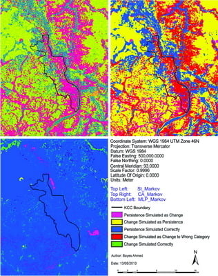
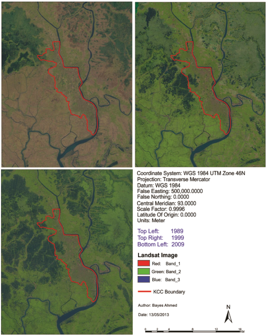
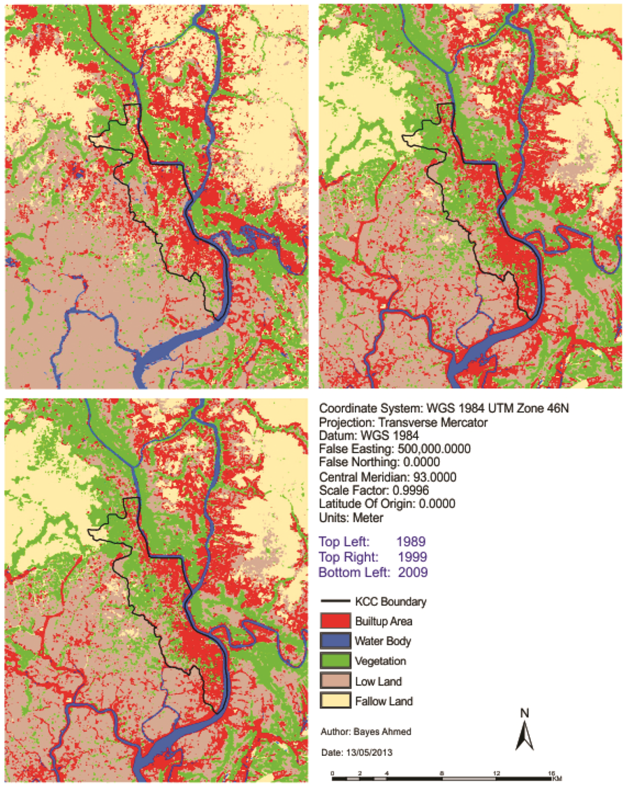
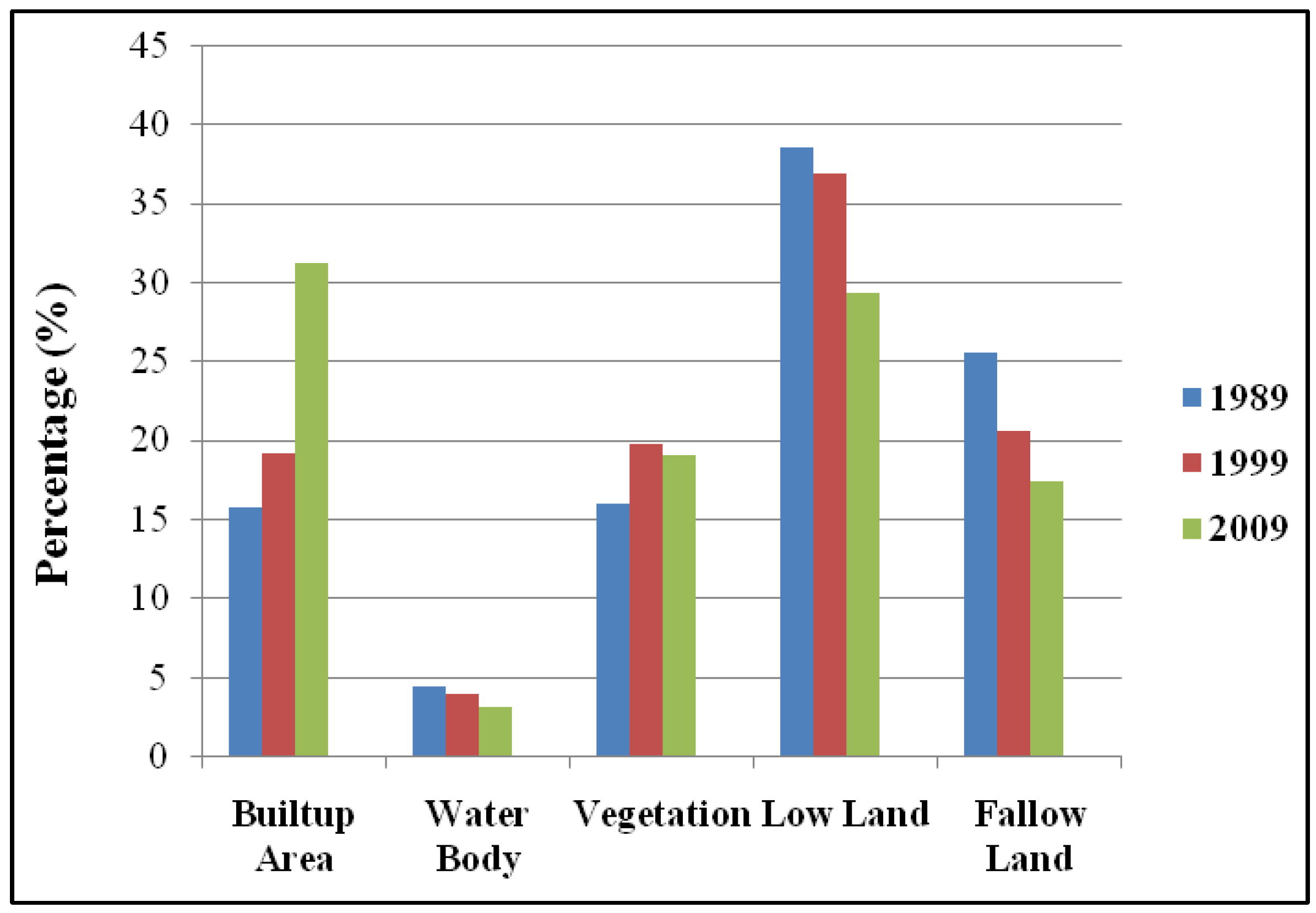
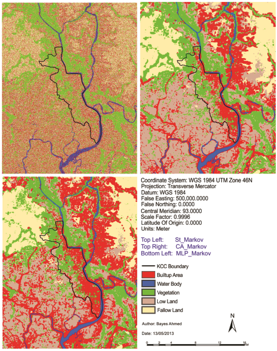
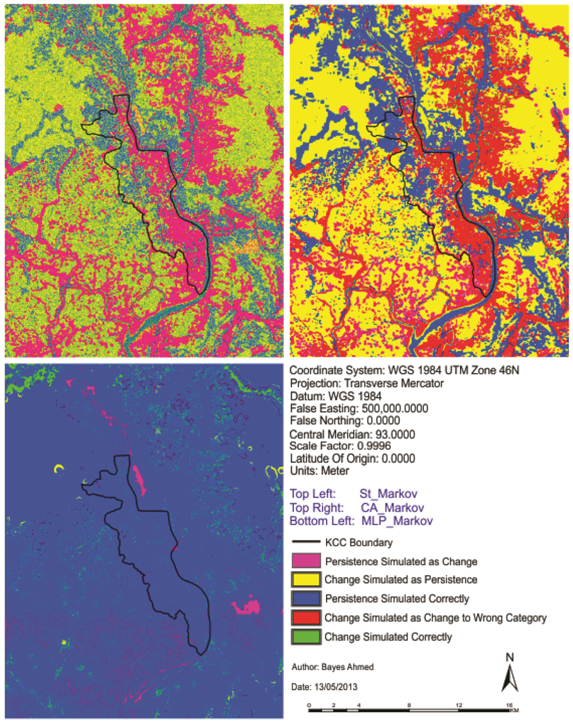
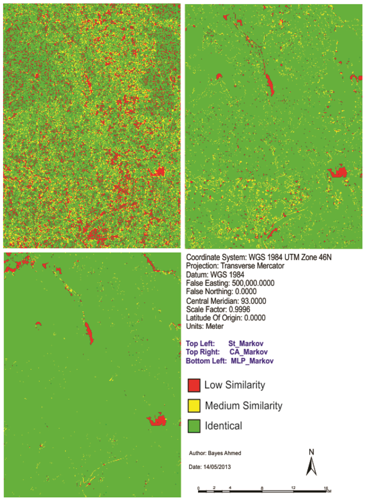
At the beginning of this paper, a fisher supervised classification method is applied to prepare the base maps of Khulna City with five land cover classes. After performing accuracy assessment and quantifying map errors, it is found that the errors in the maps are not much larger than the amount of land change between the two points in time (1989–1999 and 1999–2009). Later, being persistent with the inherent changing characteristics, three different methods are implemented to simulate the land cover maps of Khulna City (2009). The methods are named as “Stochastic Markov (St_Markov)”, “Cellular Automata Markov (CA_Markov)” and “Multi Layer Perceptron Markov (MLP_Markov)” model.
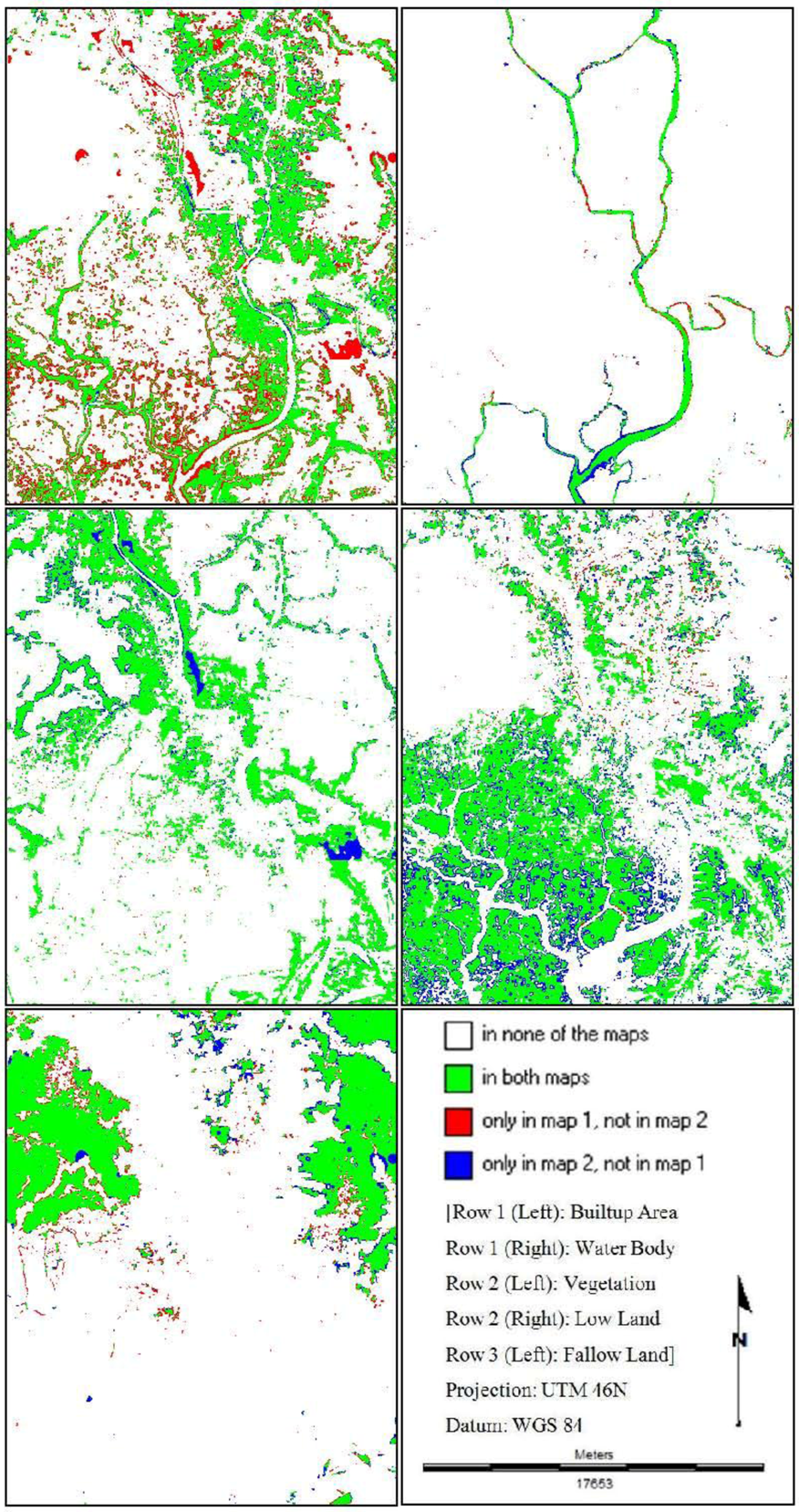
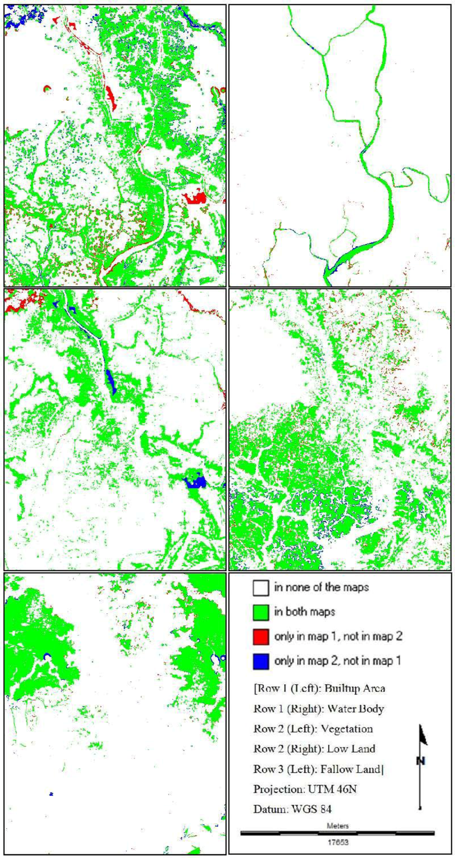
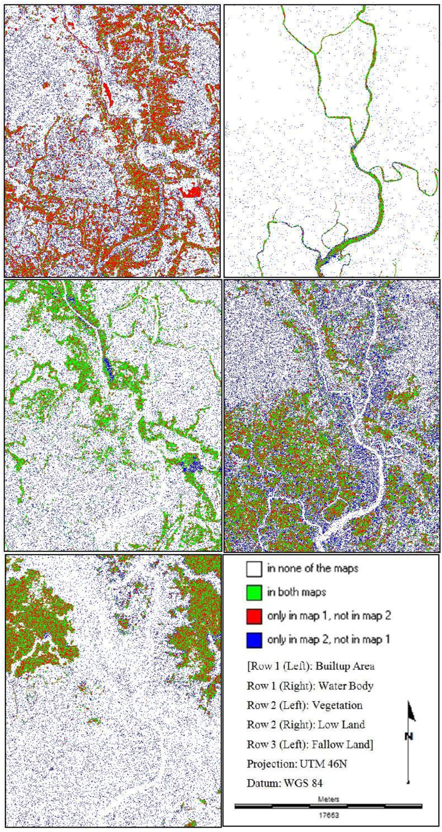
Then different model validation techniques like per category method, kappa statistics, components of agreement and disagreement, three map comparison and fuzzy method are applied. A comparative analysis, in terms of concerned advantages and disadvantages, on the validation techniques has also been discussed. Fuzzy set theory is found best able to distinguish areas of minor spatial errors from major spatial errors. In all cases, it is found that “MLP_Markov” is giving the best results among the three modeling techniques. This is how, it is possible to compare different models and choose which modeling technique is giving better results.
In order to compare the predicted change to the observed change and to perform validation for predictive land change models; it is recommended that scientists should use Kappa, three map comparison and fuzzy method based on the outcome of this paper.
Our hope might be realized if the error in the base maps is reduced to the point where the error becomes smaller than apparent change in land. This paper will help the researchers deciding whether the most important errors are in the model or in the data. Moreover, it is our belief that this kind of research has a high potential to contribute towards learning about the different available validation techniques and to choose the right one by the researchers working on different case studies.
We have designed this article in such an order so that it produces helpful information for other scientists whose goals are to validate a model’s performance and to set an agenda for future research.

5. Future Research

For any kind of model validation or map comparison, the accuracy of the base maps is very important. However, maintaining accuracy of the base maps is difficult due to lack of availability of historical data or verification of the older maps. Moreover, there are different image classification (e.g., supervised, unsupervised, object-based, hybrid, etc.) methods, which can give different results. Even the use of different filtering techniques (e.g., median, mode, mean, Gaussian), filter size, classifier (e.g., hard, soft, segmentation) and reclassification methods can give variant results. The spatial and temporal resolution of the remotely sensed images can also put impact while identifying training sites for signature development. All these factors can play important role in assessing the accuracy of maps or model validation purposes. This is why future research can be conducted incorporating all these relevant issues.
There are many available map comparison techniques. Each has its own advantages and disadvantages. Therefore, it is very important to distinguish which technique is suitable for a particular context or case study. This can be another dimension for future research. Finally, future research must address the spatial dependency between the maps to be compared.

Acknowledgments

The authors would like to express gratitude to the Department of Geography & Environmental Studies, Rajshahi University, Bangladesh for providing the GIS software ArcGIS 10® and IDRISI Selva®.
The corresponding author would also like to thank Monash University, Australia for proving necessary fund and other facilities to conduct this research. The fund has been allocated through Monash International Postgraduate Research Scholarship (MIPRS) and Monash Graduate Scholarship (MGS).
Finally, we thank the three anonymous reviewers and the editors of ISPRS IJGI for their constructive comments that improved the quality of this paper.

Conflict of Interest

The authors declare no conflict of interest.

References

  1. Pontius, R.G., Jr.; Boersma, W.; Castella, J.-C.; Clarke, K.; de Nijs, T.; Dietzel, C.; Duan, Z.; Fotsing, E.; Goldstein, N.; Kok, K.; et al. Comparing the input, output, and validation maps for several models of land change. Ann. Reg. Sci. 2008, 42, 11–47. [Google Scholar] [CrossRef]
  2. Chen, H.; Pontius, R.G., Jr. Diagnostic tools to evaluate a spatial land change projection along a gradient of an explanatory variable. Landsc. Ecol. 2010, 25, 1319–1331. [Google Scholar] [CrossRef]
  3. Visser, H.; de Nijs, T. The map comparison kit. Environ. Model. Softw. 2006, 21, 346–358. [Google Scholar] [CrossRef]
  4. Pontius, R.G., Jr.; Walker, R.; Yao-Kumah, R.; Arima, E.; Aldrich, S.; Caldas, M.; Vergara, D. Accuracy assessment for a simulation model of Amazonian deforestation. Ann. Assn. Amer. Geogr. 2007, 97, 677–695. [Google Scholar] [CrossRef]
  5. Hagen, A. Fuzzy set approach to assessing similarity of categorical maps. Int. J. Geogr. Inf. Sci. 2003, 17, 235–249. [Google Scholar] [CrossRef]
  6. Metternicht, G. Change detection assessment using fuzzy sets and remotely sensed data: An application of topographic map revision. ISPRS J. Photogramm. 1999, 54, 221–233. [Google Scholar] [CrossRef]
  7. Boots, B.; Csillag, F. Categorical maps, comparisons, and confidence. J. Geograph. Syst. 2006, 8, 109–118. [Google Scholar] [CrossRef]
  8. Hagen-Zanker, A. An improved Fuzzy Kappa statistic that accounts for spatial autocorrelation. Int. J. Geogr. Inf. Sci. 2009, 23, 61–73. [Google Scholar] [CrossRef]
  9. Richter, O.; Söndgerath, D. Parameter Estimation in Ecology: The Link between Data and Models; VCH Publishers: New York, NY, USA, 1990. [Google Scholar]
  10. Gardner, R.; Urban, D. Model Validation and Testing: Past Lessons, Present Concerns, Future Prospects. In Models in Ecosystem Science; Canham, C.D., Cole, J.J., Lauenroth, W.K., Eds.; Princeton University Press: Princeton, NJ, USA, 2004; pp. 184–203. [Google Scholar]
  11. Pontius, R.G., Jr.; Silvia, H.P. Assessing a predictive model of land change using uncertain data. Environ. Model. Softw. 2010, 25, 299–309. [Google Scholar] [CrossRef]
  12. Van Rompaey, A.J.J.; Govers, C. Data quality and model complexity for regional scale soil erosion prediction. Int. J. Geogr. Inf. Sci. 2002, 16, 663–680. [Google Scholar] [CrossRef]
  13. Foody, G.M. The impact of imperfect ground reference data on the accuracy of land cover change estimation. Int. J. Remote Sens. 2009, 30, 3275–3281. [Google Scholar] [CrossRef]
  14. Rykiel, E.J. Testing ecological models: The meaning of validation. Ecol. Model. 1996, 90, 229–244. [Google Scholar] [CrossRef]
  15. Vliet, J.V.; Bregt, A.K.; Hagen-Zanker, A. Revisiting Kappa to account for change in the accuracy assessment of land-use change models. Ecol. Model. 2011, 222, 1367–1375. [Google Scholar] [CrossRef]
  16. Hagen-Zanker, A.; Martens, P. Map Comparison Methods for Comprehensive Assessment of Geosimulation Models. In Proceedings of the International Conference on Computational Science and Its Applications, Perugia, Italy, 30 June–3 July 2008; Gervasi, O., Murgante, B., Lagana, A., Taniar, D., Mun, Y., Gavrilova, M., Eds.; Springer: Berlin, Germany; pp. 194–209.
  17. Jensen, J.R.; Ramsey, E.W.; Halkard, E.M.; Christensen, E.J.; Sharitz, R.R. Inland wetland change detection using aircraft MSS data. Photogramm. Eng. Remote Sensing 1987, 53, 521–529. [Google Scholar]
  18. Power, C.; Simms, A.; White, R. Hierarchical fuzzy pattern matching for the regional comparison of land use maps. Int. J. Geogr. Inf. Sci. 2001, 15, 77–100. [Google Scholar] [CrossRef]
  19. White, R.; Engelen, G.; Injee, I. The use of constrained cellular automata for high-resolution modelling of urban land use dynamics. Environ. Plan. 1997, 24, 323–343. [Google Scholar]
  20. Hagen-Zanker, A.; Lajoie, G. Neutral models of landscape change as benchmarks in the assessment of model performance. Landscape Urban Plan. 2008, 86, 284–296. [Google Scholar] [CrossRef]
  21. Fewster, R.M.; Buckland, S.T. Similarity indices for spatial ecological data. Biometrics 2001, 57, 495–501. [Google Scholar] [CrossRef]
  22. Ebert, E.E.; McBride, J.L. Verification of precipitation in weather systems: Determination of systematic errors. J. Hydrol. 2000, 239, 179–202. [Google Scholar] [CrossRef]
  23. Pijanowski, B.C.; Brown, D.G.; Shellito, B.A.; Manik, G.A. Using neural networks and GIS to forecast land use changes: A land transformation model. Comput. Environ. Urban Syst. 2002, 26, 553–575. [Google Scholar] [CrossRef]
  24. Briggs, W.M.; Levine, R.A. Wavelets and field forecast verification. Mon. Weather Rev. 1997, 125, 1329–1341. [Google Scholar] [CrossRef]
  25. Barredo, J.I.; Demicheli, L. Urban sustainability in developing countries’ megacities: Modelling and predicting future urban growth in Lagos. Cities 2003, 20, 297–310. [Google Scholar] [CrossRef]
  26. Turner, M.G.; Costanza, R.; Sklar, F.H. Methods to evaluate the performance of spatial simulation-models. Ecol. Model 1989, 48, 1–18. [Google Scholar] [CrossRef]
  27. Urban Strategy. In Structure Plan, Master Plan and Detailed Area Plan (2001–2020) for Khulna City; Aqua-Sheltech Consortium, Khulna Development Authority: Khulna, Bangladesh, 2002; Volume I.
  28. Ahmed, B.; Ahmed, R. Modeling urban land cover growth dynamics using multi-temporal satellite images: A case study of Dhaka, Bangladesh. ISPRS Int. J. Geo-Inf. 2012, 1, 3–31. [Google Scholar] [CrossRef]
  29. Liu, H.; Zhou, Q. Accuracy analysis of remote sensing change detection by rule-based rationality evaluation with post-classification comparison. Int. J. Remote Sens. 2004, 5, 1037–1050. [Google Scholar] [CrossRef]
  30. Eastman, J.R. IDRISI Taiga Guide to GIS and Image Processing, Manual Version 16.02 (Software); Clark Labs: Worcester, MA, USA, 2009. [Google Scholar]
  31. Basharin, G.P.; Langville, A.N.; Naumov, V.A. The life and work of A.A. Markov. Linear Algebr. Appl. 2004, 386, 3–26. [Google Scholar] [CrossRef]
  32. Weng, Q. Land use change analysis in the Zhujiang Delta of China using satellite remote sensing, GIS and stochastic modelling. J. Environ. Manage. 2002, 64, 273–284. [Google Scholar] [CrossRef]
  33. Maerivoet, S.; Moor, B.D. Cellular automata models of road traffic. Phys. Rep. 2005, 419, 1–64. [Google Scholar] [CrossRef]
  34. Malczewski, J. GIS-based land-use suitability analysis: A critical overview. Prog. Plan. 2004, 62, 3–65. [Google Scholar] [CrossRef]
  35. Karul, C.; Soyupak, S. A Comparison between Neural Network Based and Multiple Regression Models for Chlorophyll-A Estimation. In Ecological Informatics; Recknagel, F., Ed.; Springer: Berlin, Germany, 2006; pp. 309–323. [Google Scholar]
  36. Atkinson, P.M.; Tatnall, A.R.L. Introduction neural networks in remote sensing. Int. J. Remote Sens. 1997, 18, 699–709. [Google Scholar] [CrossRef]
  37. Vliet, J.V. Map Comparison Kit 3 User Manual, Manual Version 3.2 (Software); Research Institute for Knowledge Systems BV: Maastricht, The Netherlands, 2009. [Google Scholar]
  38. Pontius, R.G., Jr. Quantification error versus location error in the comparison of categorical maps. Photogramm. Eng. Remote Sensing 2000, 66, 1011–1016. [Google Scholar]
  39. Pontius, R.G., Jr. Statistical methods to partition effects of quantity and location during comparison of categorical maps at multiple resolutions. Photogramm. Eng. Remote Sensing 2002, 68, 1041–1049. [Google Scholar]
  40. Cohen, J. A coefficient of agreement for nominal scales. Educ. Psychol. Meas. 1960, 20, 37–46. [Google Scholar] [CrossRef]
  41. Kitada, K.; Fukuyama, K. Land-use and land-cover mapping using a gradable classification method. Remote Sens. 2012, 4, 1544–1558. [Google Scholar] [CrossRef]
  42. Ahmed, B. Modelling spatio-temporal urban land cover growth dynamics using remote sensing and GIS techniques: A case study of Khulna City. J. Bangladesh Instit. Plan. 2011, 4, 16–33. [Google Scholar]
  43. Long, J.B.; Giri, C. Mapping the Philippines’ mangrove forests using landsat imagery. Sensors 2011, 11, 2972–2981. [Google Scholar] [CrossRef]
  44. Pontius, R.G., Jr.; Millones, M. Death to Kappa: Birth of quantity disagreement and allocation disagreement for accuracy assessment. Int. J. Remote Sens. 2011, 32, 4407–4429. [Google Scholar] [CrossRef]
  45. Pontius, R.G., Jr.; Millones, M. Problems and Solutions for Kappa-Based Indices of Agreement. In Proceedings of the Conference Studying, Modeling and Sense Making of Planet Earth, Mytilene, Greece, 1–6 June 2008.
  46. Pontius, R.G., Jr.; Peethambaram, S.; Castella, J.C. Comparison of three maps at multiple resolutions: A case study of land change simulation in Cho Don District, Vietnam. Ann. Assn. Amer. Geogr. 2011, 101, 45–62. [Google Scholar] [CrossRef]
  47. Singh, A. Digital change detection using remote-sensing data. Int. J. Remote Sens. 1989, 10, 989–1003. [Google Scholar] [CrossRef]
  48. Mas, J.F. Monitoring land-cover changes: A comparison of change detection techniques. Int. J. Remote Sens. 1999, 20, 139–152. [Google Scholar] [CrossRef]
  49. Jensen, J.R. Urban change detection mapping using Landsat digital data. Amer. Cartographer 1981, 8, 127–147. [Google Scholar] [CrossRef]
  50. Macleod, R.D.; Congalton, R.G. A quantitative comparison of change detection algorithms for monitoring eelgrass from remotely sensed data. Photogramm. Eng. Remote Sensing 1998, 64, 207–216. [Google Scholar]
  51. Zadeh, L.A. Fuzzy sets. Inf. Control 1965, 8, 338–353. [Google Scholar] [CrossRef]
  52. Bandemer, H.; Gottwald, S. Fuzzy Sets, Fuzzy Logic, Fuzzy Methods with Applications; Wiley: New York, NY, USA, 1995. [Google Scholar]
  53. Cheng, T.; Molenaar, M.; Lin, H. Formalizing fuzzy objects from uncertain classification results. Int. J. Geogr. Inf. Sci. 2001, 15, 27–42. [Google Scholar] [CrossRef]
  54. Lewis, H.G.; Brown, M. A generalized confusion matrix for assessing area estimates from remotely sensed data. Int. J. Remote Sens. 2001, 22, 3223–3235. [Google Scholar] [CrossRef]
  55. Hagen-Zanker, A. Comparing Continuous Valued Raster Data: A Cross Disciplinary Literature Scan; Research Institute for Knowledge Systems BV: Maastricht, The Netherlands, 2006. [Google Scholar]

