1. Introduction
In recent decades, people are more likely to use digital media or mobile devices in their daily life which consists of a series of activities, such as working, rest, shopping and recreation [
1]. The increasing pervasiveness and proliferation of location-aware sensors in these devices has left behind a massive dataset of human mobility providing a potential chance for analyzing and mining interest patterns of human activities. These patterns play an important role in our society. They help in the understanding of contemporary urbanism, and particularly they strengthen our understanding of society in place [
2]. Most importantly, they facilitate the issues of urban planning [
3], transportation [
4], infectious disease control and emergency management [
5]. Therefore, extensive research, both theoretical and empirical, is being focused on this topic.
Theoretically, as an antecedent of activity analysis, the time geography postulated by [
6] is useful in revealing the pattern of interaction between individuals and place with time, but it lacks the ability to present a more sensual and richer picture of these synchronic activities [
7]. Consequently, Edensor [
7] recommended using Rhythmanalysis [
8] to explore the everyday activities in space-time, mainly to examine how rhythms shape human activities. By observing the characteristics of activities in urban space, Gehl [
9] suggested three categories: timed social activity, optional social activity and resultant activity. Among these categories, the timed social activity constitutes a large proportion and refers to an individual constrained by institutional timetables and schedules [
10], such as going to work in the morning. Furthermore, these constraints lead to two possible patterns of human activity, namely the non-identical repetition in time and the particular place related as described by [
8]. Therefore, the purposely related taxicab data provides a good source for investigating the timed social activity.
Empirically, paper-based activity diaries [
11,
12,
13] have been adopted for obtaining information on human spatial-temporal behaviors and activities. These diaries provide detailed information on the type of activity, but are time-consuming, offering only small data samples and have a memory bias [
14]. On the other hand, voluminous mobility data can be collected by devices equipped with GPS or GSM. This inspires a renaissance on the investigation of this issue since these data are massive, convenient and even objective. For example, several previous studies [
15,
16,
17] examined the space-time dynamic of urban life for a better understanding of how a city functions. In addition, based on the aggregated level, Krygman
et al. [
14] showed the daily urban dynamic using a small sample of participants, whereas Ahas
et al. [
18] found the diurnal rhythm of city life and its spatial difference in Tallinn using a relatively large sample of participants. Furthermore, Neuhaus [
19] captured the pulse of city life in London from the perspective of an individual level. Apart from the mobile phone data, Liu
et al. [
20] also studied the space-time urban mobility patterns in Shenzhen by using the GPS based taxicab data and public transportation data.
This research differs from the above studies in two main ways. Firstly, the emphasis is put on the static points (SPs) instead of the entire tracking records, and secondly, the patterns of human activities are investigated from both the aggregated and individual level. SPs refer to locations with zero speed along the tracking trajectory. They are the locations where taxicabs stop for a while along route to the customer destination, e.g., traffic intersection, parking lot,
etc. From this point, it allows a good proxy of activities since in most cases they are associated with different types of activities. Note that we are not concerned with the type of activity associated to the location ([
12,
13,
14,
18]) but simply consider it as a general activity. With this generality, we examine the activity patterns in the case from both aggregated and individual levels. On the aggregated level, we report the findings from the temporal, spatial and scaling analysis. The temporal analysis enables us to understand the pulse of activities within the entire study area; the spatial analysis allows us to detect the pattern of activities drifting which is a topic that receives little attention; and the scaling analysis examines the diffusion characteristic of activities. On the individual level, this paper firstly examines the activity pattern of each taxicab, and then we report findings on predictability, for example, how much information is needed to describe the next activity location.
The remainder of this paper is organized as follows. In
Section 2, we describe the data adopted and the corresponding procedure to extract the SPs. In
Section 3, we report the main findings, namely the patterns of human activities from the temporal, spatial and scaling analyses. In
Section 4, we present the pattern and the ensuing predictability of individual taxicabs. Finally, we draw a conclusion in
Section 5.
3. Analysis of Human Activities from the Aggregated Perspective
This section aims to examine the overall patterns of human activities in the study area. We firstly report the result of the temporal pattern in the entire study region, and thereafter we present the spatial drifting pattern from one district to another. Finally, we carry out a scaling analysis on the diffusion pattern of activities in the study region.
3.1. Temporal Analysis
Time cycles regularly in terms of 24 h a day for all individuals in every part of the world. Following this regularity, everyone participates in a series of activities (e.g., sleeping, waking,
etc.). However, this activity-sequence varies with different customs, albeit that there is little fluctuation among individuals in the same city. For example, the Swedes celebrate Christmas Eve with their families staying at home, whereas during the New Year Eve they, particularly the young people, are more likely to go out to count down to the coming new year with their friends (Source:
www.sweden.se). From this point, it can be seen that time plays an important role in shaping activities.
Besides, as noted by [
21] human society is formed by the sequence of activities performed by individuals, the aggregated individual activities reflect the overall pattern for a particular society. Bearing this idea in mind, we coin a term city time spectrum (CTS) illustrating activities changing with time. In CTS, the x-axis represents the hours in one day, the y-axis represents the dates and each cell reflects the intensity of activities which can be defined from the perspective of SPs volume or wait time, e.g.,
![Ijgi 01 00089 i008]()
or
![Ijgi 01 00089 i009]()
. This kind of analysis is similar to the concept of real time-use in time geography proposed by [
22], but with the emphasis on the entire urban area.
As shown in
Figure 4(a,b), the CTS clearly reveal the activity patterns. During the weekdays, we can observe that: (1) there is a burst of human activities from 07:00 to 17:00; and (2) there is a lull in human activities from 18:00 to 06:00. However, on the weekends, it displays the converse situation. Besides, CTS can uncover contextual information of a particular city which shows how it differs from others. For example, nights on the weekend is clearly depicted as high intensity in
Figure 4(a) while low intensity in
Figure 4(b), which generally reflects the distinct culture of the local society. Particularly, the red color cell in
Figure 4(a) at 02:00 on 28 October uncovers the burst of activities due to the Halloween weekend. Apart from the CTS analysis, we further illustrate this phenomenon in
Figure 4(c,d) where the periods of relative bursts or silences of human activities are identified for both weekdays and weekends. These specific periods not only reveal the regularity of activities, but also are useful for traffic control and management.
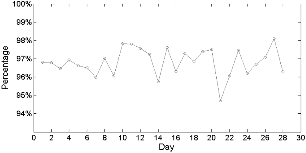
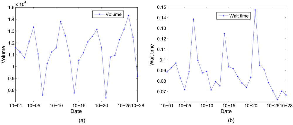
To further explore the pattern of human activities, we present the changes of the two properties, volume and wait time, with time on a daily basis in
Figure 5. It clearly shows that human activities repeat a high degree of regularity from one week to another: It reaches a peak on Friday but dips on a Sunday. The peak on Fridays can be attributed to extra outings, people go to the pub during the night or travel away for the weekend. On the other hand, the dip on Sunday is reasonable since we usually want to have a rest on this day, preparing for the coming week. However, a relative high value in SPs volume or low value in SPs wait time is observed on 28 October, which can also be attributed to the Halloween weekend.
Figure 4.
Human activities changing on an hourly basis (Note: (a) shows the CTS for SPs volume, where we can clearly observe the activities pattern of the local residents repeats daily and weekly. Worthy of note is that the date 07-10-07 was a Sunday; (b) demonstrates the CTS for SPs wait time, where the pattern exhibits the opposite characteristic as that shown in (a); (c) plots hourly based change of average SPs volume on weekdays and weekends respectively, and the dot-box represents the period of relative bursts or silence of activities; (d) plots the hourly based change of the average SPs wait time on weekdays and weekends respectively but displays an opposite trend to (c)).
Figure 5.
Plot of human activities changing on a daily basis (Note: These uncover the periodic regularity of activities on a daily basis. To be specific: (a) reflects this regularity from the SPs volume; (b) reveals this pattern from the SPs wait time, which depicts the same regularity from the opposite viewpoint).
3.2. Spatial Analysis
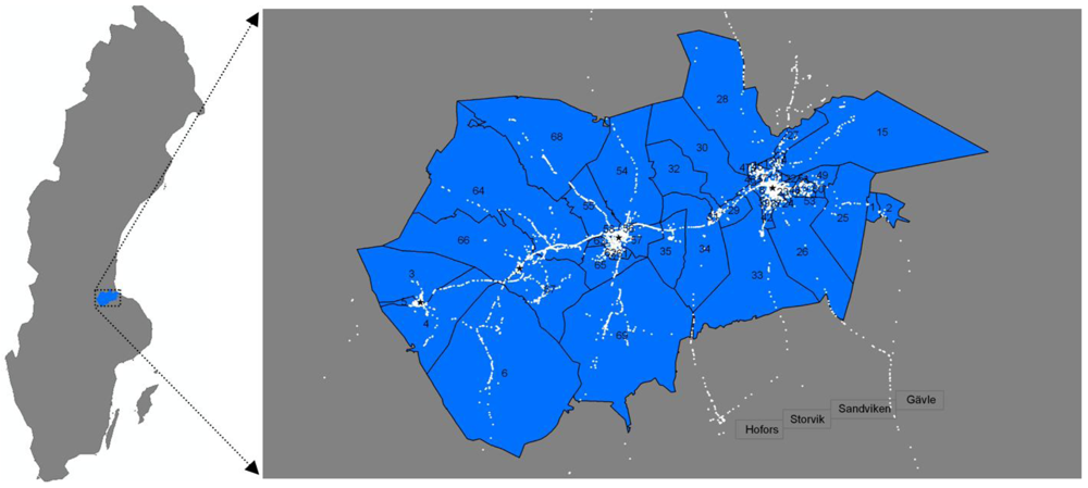
The temporal analysis shows that human activities surge during certain periods, whereas they disappear in others. However, this does not tell us which region of the city is in vitality or in silence. In other words, we need to explore how activities drift in space. To answer this question and for the simplicity of analysis, we adopt the 69 city districts in the study area as the basic spatial units. These spatial units represent an administrative demarcation of the study area, and they reflect the underlying contextual information of each district, such as land use type and population. Therefore, our problem has been simply converted to answer the question of how activities drift among the city districts.
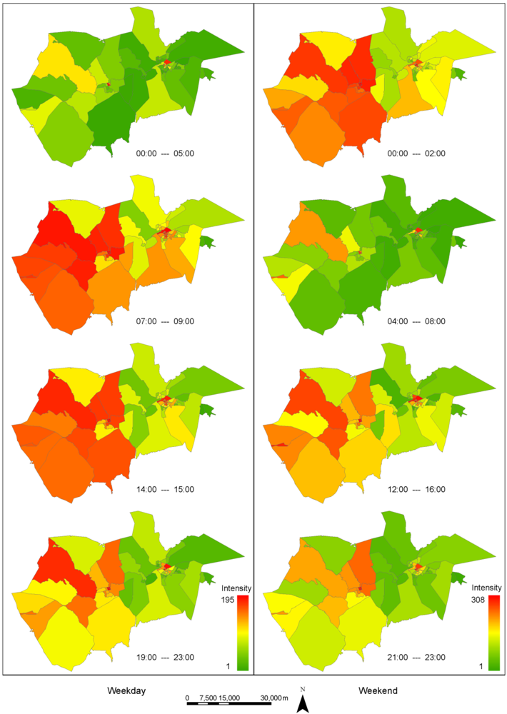
To cope with this problem, we assign the intensity of activities to each city district. The intensity value here is measured by the average volume of SPs for one month, and we firstly take a look at how the activities intensity changes in space on an hourly basis. As shown in
Figure 6, we present the map of the activities intensity drifting in 69 city districts within four peak periods on both weekdays and weekends. Note that different city districts are depicted by different colors according to the value of the intensity, and can be compared with each other across four different peak periods because of our uniform rendering strategy. The pattern of the weekday spatial drifting suggests that: the activities are mainly concentrated in the city central districts during the small hours, and then there is a burst and expansion towards the surrounding districts during the morning period, which can be observed easily in the three districts adjacent to the Sandviken central district in which the largest Swedish high-technology engineering company Sandvik (Source:
http://en.wikipedia.org/wiki/Sandvik) is located. In the afternoon, most districts remain stable except for a small decrease around the Gävle central districts, and then a major decrease in all city central districts in the evening.
However, the pattern of the weekend spatial drifting tells a different story. The activities surge and spread across the central and surrounding districts from 00:00 to 02:00, which reflects the night life of the local residents, followed by a reduction and contraction to a few central districts from 04:00 to 08:00. During the afternoon, there is an increase and expansion in the neighboring districts, which is followed by a minor decrease in the central districts in the evening. From the above description, two facts can be identified. First, the spatial drifting pattern is different from weekdays to weekends, which is highly associated with the life style of the local residents. Second, the total intensity of human activities is proportional to the extent of spatial diffusion and is mainly concentrated on very few central districts.
Figure 6.
Map of the intensity of activities changing with time on an hourly basis.
Figure 6.
Map of the intensity of activities changing with time on an hourly basis.
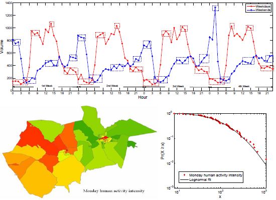
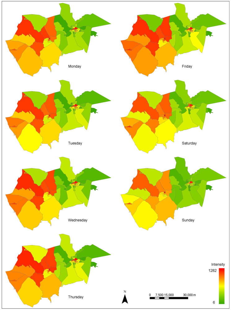
To take the investigation a step further, we examine the spatial drifting pattern on a daily basis from Monday to Sunday. As shown in
Figure 7, there is significant regularity of activities intensity for each district from Monday to Sunday, although there are small fluctuations in very few districts. Besides, each city or town has its own pattern of diffusion among its districts which keeps relatively stable on a daily basis from Monday to Sunday. For example, activities are more concentrated in the northern districts of Gävle city. Finally, we can observe that activities are more diffused on Friday and less diffused on Sunday, which is in agreement with our report in
Figure 5.
Figure 7.
Map of the intensity of activities changing with time on a daily basis.
Figure 7.
Map of the intensity of activities changing with time on a daily basis.
Unlike the temporal analysis which investigates the entire region, the spatial analysis allows us to delve into the individual spatial unit and examine the drifting of human activities from one unit to another. In this respect, it not only strengthens our understanding of the activities in place [
8], but also helps us in many other fields, such as disease control, traffic management and city planning. For example, an important issue in city planning is to investigate the mutual relationship between the human activities and the urban landscape, and our conjecture is that the spatial drifting pattern may help to establish this relationship: through the correlation analysis of the intensity of human activities within the spatial unit with the different landscape metrics of the spatial unit, it may be possible to build a mathematical model to explain this mutual relationship. Besides, our finding suggests that the activities are more concentrated in a few districts irrespective of their drifting in space with time. This fact hints that very few districts act as attractors of human activities whereas others are rarely visited, and this fact is further analyzed in the following section.
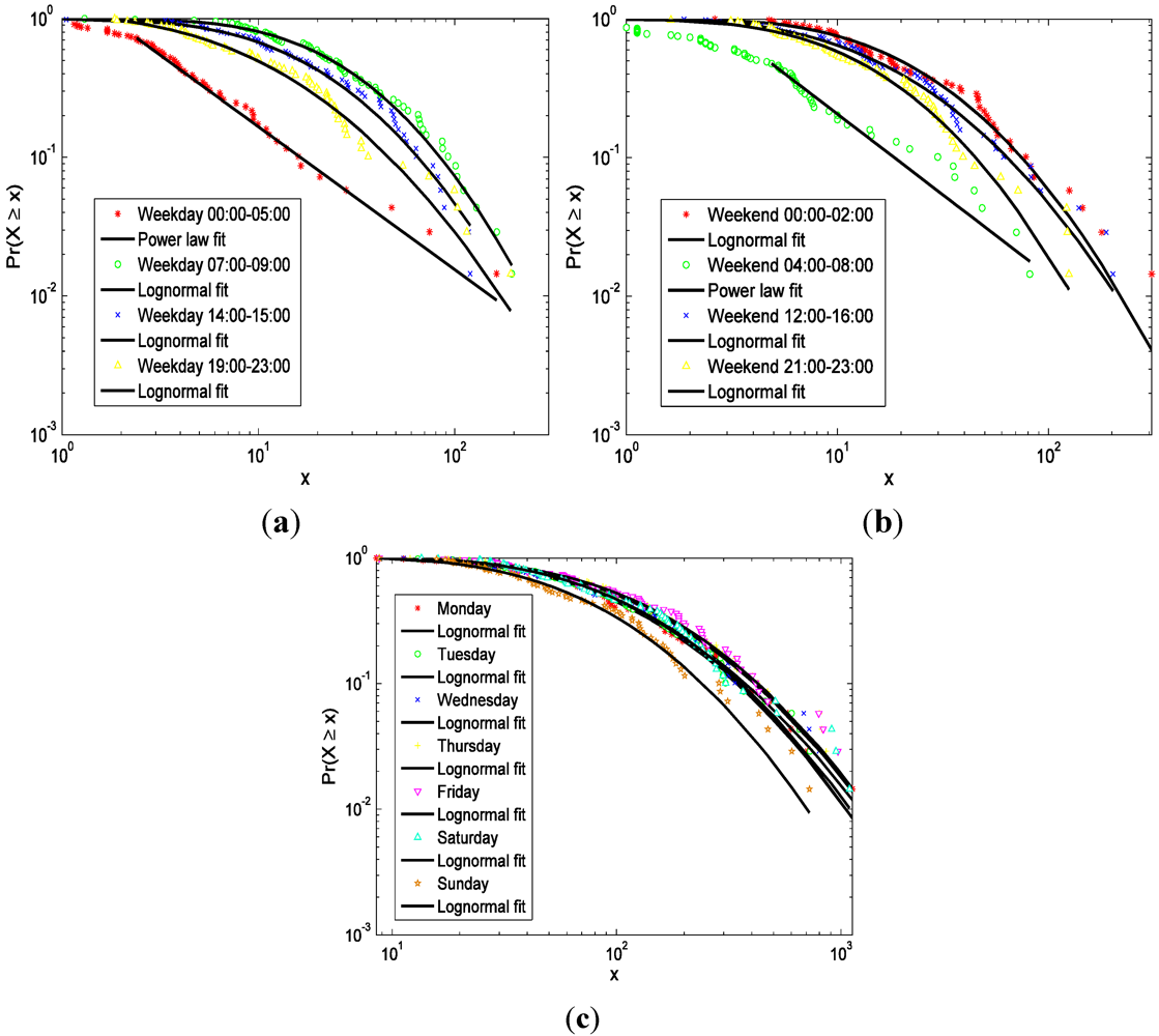
3.3. Scaling Analysis
To support the above viewpoint, we conducted a scaling analysis. The aim is to identify whether the property of a phenomenon follows a heavy-tailed distribution. The detailed procedure is specified in [
23,
24,
25]. A heavy-tailed distribution indicates that there are far more small ones than large things [
26], and includes the distributions of power law, lognormal, stretched exponential, power law with cutoff, and so on [
23]. In this study, we find that the intensity of human activities agrees well with the power law (
![Ijgi 01 00089 i010]()
) or lognormal (
![Ijgi 01 00089 i011]()
) distribution with high
p-value passing the KS test [
23] on either an hourly or a daily basis (
Figure 8,
Table 1 and
Table 2). Importantly, the intensity of human activities during the rest periods (from 00:00 to 05:00 on weekdays and from 04:00 to 08:00 on the weekend) can be well approximated by the power law distributions, whereas all others agree well with the lognormal distributions. Moreover, here the power law distribution appears much more heterogeneous than the lognormal distribution, which can also be well observed in
Figure 6.
Figure 8.
The plot for the heavy-tailed distribution of the intensity of human activities (Note: on an hourly basis, (a) shows weekdays; and (b) weekends; on a daily basis; (c) displays the plot from Monday to Sunday).
Figure 8.
The plot for the heavy-tailed distribution of the intensity of human activities (Note: on an hourly basis, (a) shows weekdays; and (b) weekends; on a daily basis; (c) displays the plot from Monday to Sunday).
Table 1.
Heavy-tailed distribution of human activities on an hourly basis.
Table 1.
Heavy-tailed distribution of human activities on an hourly basis.
| | Period | Model | Parameters | P |
|---|
| Weekday | 00:00–05:00 | power law | α = 2.03 | 0.7 |
| 07:00–09:00 | lognormal | μ = 3.16, σ = 0.99 | 0.7 |
| 14:00–15:00 | lognormal | μ = 2.79, σ = 1.08 | 0.1 |
| 19:00–23:00 | lognormal | μ = 2.11, σ = 1.28 | 0.1 |
| Weekend | 00:00–02:00 | lognormal | μ = 2.96, σ = 1.05 | 0.1 |
| 04:00–08:00 | power law | α = 2.17 | 0.2 |
| 12:00–16:00 | lognormal | μ = 2.67, σ = 1.15 | 0.7 |
| 21:00–23:00 | lognormal | μ = 2.51, σ = 1.01 | 0.7 |
Table 2.
Heavy-tailed distribution of human activities on a daily basis.
Table 2.
Heavy-tailed distribution of human activities on a daily basis.
| | Model | Parameters | P |
|---|
| Monday | lognormal | μ = 4.45, σ = 1.08 | 0.7 |
| Tuesday | lognormal | μ = 4.50, σ = 1.06 | 1.0 |
| Wednesday | lognormal | μ = 4.45, σ = 1.13 | 0.9 |
| Thursdays | lognormal | μ = 4.59, σ = 1.10 | 1.0 |
| Friday | lognormal | μ = 4.66, σ = 1.08 | 0.6 |
| Saturday | lognormal | μ = 4.47, σ = 1.08 | 0.3 |
| Sunday | lognormal | μ = 4.14, σ = 1.04 | 0.4 |
Until now we have reported the heavy-tailed distribution for the intensity of human activities, and it implies that few districts are highly visited whereas most are rarely visited. In fact, this phenomenon has also been reported from many other aspects of the geographical space, such as the city street [
27] and city block [
28]. However, the patterns from the aggregated perspective in terms of the temporal, spatial and scaling analysis do not tell the story of individual activities, for example, if they exhibit the same rhythm, if their activity pattern is random or regular, and so on.
4. Analysis of Human Activities from the Individual Perspective
To answer the questions proposed above, we concentrate our effort on the individual level in this section. Generally speaking, two issues around the patterns of individual activities are discussed. Firstly, we report the result for the pattern of individual activities. Secondly, we examine the issue of whether the mobility of individual taxicab is regular, and subsequently how much information it contains.
4.1. Pattern of Individual Taxicab
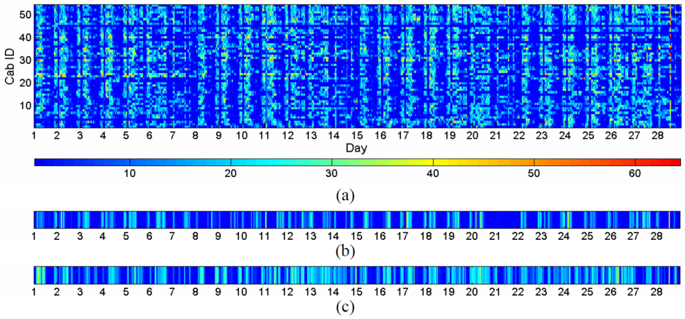
Based on the SPs of each taxicab, we derive their CTS graph as shown in
Figure 9. From the graph (
Figure 9(a)), it can be roughly seen that the activities from each taxicab show individual rhythms. For example, the activities of taxicab No.1 (
Figure 9(b)) roughly reaches its peak during the early morning but wanes in the afternoon. On the other hand, the activities of taxicab No.9 (
Figure 9(c)) surges every Friday or Saturday. In other words, a majority of taxicabs have different activity patterns from the temporal analysis.
Figure 9.
CTS for individual taxicabs (Note: in this graph, the x-axis is the time dimension with hourly units but labeled as day for clarity (e.g., 1 in x-axis is the date 2007-10-01 00:00), while y-axis represents the ID of each taxi cab; in particular, (a) shows the graph of CTS for all taxicabs; (b) is an enlarged graph of the CTS for taxicab No.1; (c) is an enlarged graph of the CTS for taxicab No.9).
To quantitatively assess the similarity among individual taxicabs, the Pearson correlation coefficient is employed on every pair of taxicabs. Here we assume the behavior of one individual taxicab is independent from another’s. As shown in
Figure 10(a), we can observe that most of the pixels appear as cool (dark or grey) colors except for a few hot (white) ones, which indicate that the R-Square values for most of taxicab pairs are very small with a few exceptions. Moreover, the empirical distribution function in
Figure 10(b) indicates that more than 90% of the total number of taxicab pairs has an R-Square value of less than 0.2. Therefore, it is concluded that most of the taxicabs have an activity pattern that is different another’s. This finding is self-evident because every taxicab driver has his or her own time schedule of running the business for the sake of competition. For example, a taxi driver during a certain period would chose places where they have a bigger chance of getting custom.
Figure 10.
R-Square values for the pairs of taxicabs (Note: (a) shows image of R-Square values for every pair of taxicabs, where both x-axis and y-axis denote the taxicab ID; (b) is the empirical distribution function for all the R-Square values).
Figure 10.
R-Square values for the pairs of taxicabs (Note: (a) shows image of R-Square values for every pair of taxicabs, where both x-axis and y-axis denote the taxicab ID; (b) is the empirical distribution function for all the R-Square values).
4.2. Information of Individual Taxicabs
The above analysis suggests that the activities of individual taxicabs obey a certain degree of temporal rhythm, but it does not tell the regularity of individual taxicabs moving in space. Exploring the pattern of individual activities in the spatial context is not only helpful for deeply understanding the rhythm of individual taxicabs, but also useful for public transportation design and management. However, it is extremely difficult to examine this issue on the granularity of latitude-longitude. In other words, this issue is highly related to the Modifiable Area Unit Problem (MAUP) [
29] which will not be evaluated here. For example, it is very easy to estimate the next location if the spatial unit is the entire study region, but the situation would be very hard if the spatial unit is at latitude-longitude level since we can never estimate the next location accurately. In this study, we adopt the 69 city districts as the basic spatial units, and particularly we also include the space beyond the study area as one spatial unit to cover all SPs. Thereafter, the entire space is divided into 70 spatial units covering 69 city districts and 1 outside space.
In addition, the activity path of taxicab
i can be described as an ordered string
![Ijgi 01 00089 i012]()
, where each item represents the coding symbol of the underlying spatial unit within which the current activity is taking place. To examine the patterns in the path string, the conventional method is based on Shannon [
30] entropy which is a measurement of information within a system. Here, three typical methods are employed to quantify the information within a sequence of symbols. The first one is called the random entropy which is defined as
![Ijgi 01 00089 i013]()
, where N is the number of distinct symbols (spatial units) a path string (taxicab) has (visited). The random entropy treats every spatial unit as having the same visiting probability but ignores both the spatial (visiting frequency) and the temporal (visiting sequence) order of the visited regions. The order entropy is defined as
![Ijgi 01 00089 i014]()
, where
pj is the probability of spatial unit j being visited. It considers the spatial order namely every region has different visiting probability, but it does not take into account the temporal order.
The latter, considering both the spatial and temporal order, is termed as real entropy which is based on the Lempel-Ziv data compression algorithm. It is a kind of lossless data compression method using a dictionary, and it is proven to converge to the true entropy of a time series by [
31]. Although there are many versions of definitions for this entropy, we adopt the definition given by [
32] for the similarity of research,
![Ijgi 01 00089 i015]()
where ki is the length of the path string for taxicab i, Li is the shortest length of substring starting from position j that does not match any substrings within the window from position 1 to j-1. Here, considering two extreme cases, in the case of the Path(i) with ki same symbols, the real entropy is calculated as 2*log2ki/ki + 1, which converges to 0 as ki→∞. In another case where the Path(i) with ki different symbols, the real entropy is Log2ki, which is the same as the random and order entropy. From this perspective, the real entropy is more reasonable in reality as it sets a lower boundary for the information.
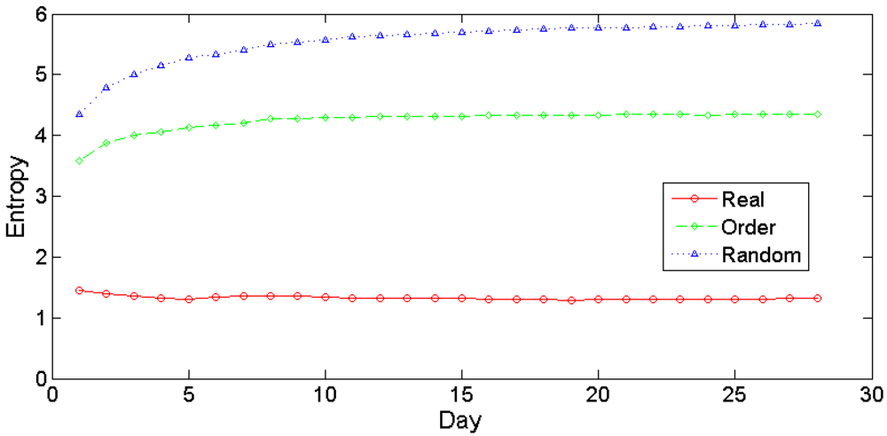
We show the changes of average entropy as the size of activity path culminates with time in
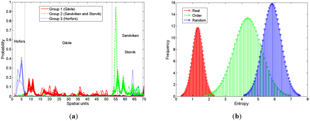
Figure 11, and it is observed that all three kinds of entropy reach equilibrium at the end of the month. This finding justifies the feasibility of using the size of one month data to examine the current issue. Based on this finding, we plot the activities probability distribution among the 70 spatial units for each taxicab in
Figure 12(a). From this figure, we can understand the activity behavior of individual taxicabs in space. One is that the taxicabs are demarcated into three groups: taxicabs servicing in Gävle, in Sandviken and Storvik, and in Hofors. The other one is that there is a large difference of visiting frequency among the 70 spatial units for each taxicab, e.g., few spatial units are highly visited while most are rarely visited. Generally, the two facts hint that the activities of individual taxicabs are highly regular in space, and hence it is theoretically predictable with little information.
Figure 11.
The plot for the trend of average entropy with time.
Figure 11.
The plot for the trend of average entropy with time.
Figure 12.
The plot for (a) activities distribution in space and (b) their entropy distributions.
Figure 12.
The plot for (a) activities distribution in space and (b) their entropy distributions.
To demonstrate the information obtained from individual taxicabs, we plot their entropy distributions in
Figure 12(b). It is found that all three distributions follow a Gaussian bell-shape, which indicates most taxicabs are more likely to visit the region which has been highly visited in history. Importantly, the distributions of real entropy, order entropy and random entropy are around the value of 1 bit, 3 bits and 5 bits respectively. The value of 1 bit information to estimate the next location of activity further demonstrates the significant regularity of individual taxicabs in space, although the rhythm for individual taxicabs in time differs from one to another as examined previously.
5. Conclusions
In this paper, we have investigated the human activity patterns through the adoption of taxicab SPs. Findings from the temporal analysis show that the overall patterns of activities exhibit an obvious regularity either on an hourly based evolution within a day or on a daily based evolution within a month. These temporal patterns not only uncover contextual knowledge of the local society, but also are useful for traffic control and management. Besides, results from the spatial analysis reveal the patterns of activities drifting across the 69 city districts, which strengthen our understandings on place and further helps urban planning and management. Moreover, we conducted a scaling analysis on the intensity of activities in each district, and we report its heterogeneous characteristics irrespective of the specified time periods. Interestingly, activities during the rest periods appear much more heterogeneous than in other periods.
This study further presents the regularity of activities of individual taxicabs. Based on the matrix of Pearson correlation coefficients, we report that there is a large diversity among the activity patterns of individual taxicabs in time, although each one has its own temporal rhythm suggesting a bottom up self-organizing procedure of the aggregated temporal rhythm. On the other hand, inspired by the temporal regularity of individual taxicabs, we find that the entropy distribution of all taxicabs follows a normal distribution, the mean value of which further reveals an average of 1 bit information is needed to estimate the next activity location.
The novel idea of adopting trajectory SPs as the proxy of human activities allows us to conveniently analyze and explore their patterns in geographical space. In this respect, our study adds another possible strategy apart from the conventional way of examination requiring the recording of human activity in space. Furthermore, it is our belief that the SPs should match well with the underlying spatial point of interests, and this reflects the basis of our future study.


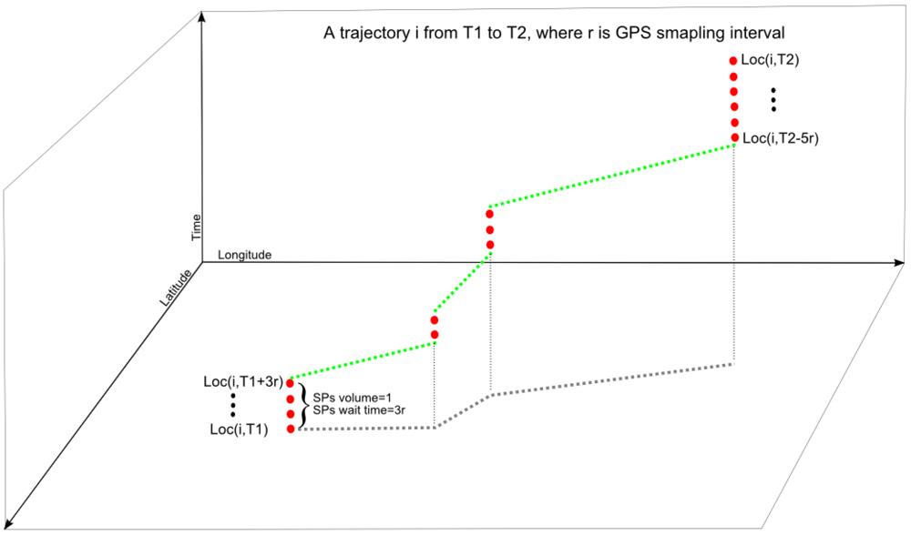
 , which is a sequence of time-stamped locations. It naively reflects all the mobility characteristics of a taxicab no matter whether it is in-service or out-of-service. Therefore, in this context, there are 54 trajectories since each object has only one trajectory within the period.
 , we devise two variables to describe them. One is the SPs volume
  , which represents the number of distinct static points for trajectory i from time T1 to T2. The other one is the SPs wait time
  which means the average time duration of the distinct static points of a trajectory i from T1 to T2. Obviously, both of the two properties can reflect the activity status but from a converse perspective. For example, a high value of SPs volume within a particular period reflects the burst of human activities while a high value of SPs wait time represents a silent situation. Generally, they are denoted as,
 is the jth static point for trajectory i, and ki is the number of static points of trajectory i.

 or
or  . This kind of analysis is similar to the concept of real time-use in time geography proposed by [22], but with the emphasis on the entire urban area.
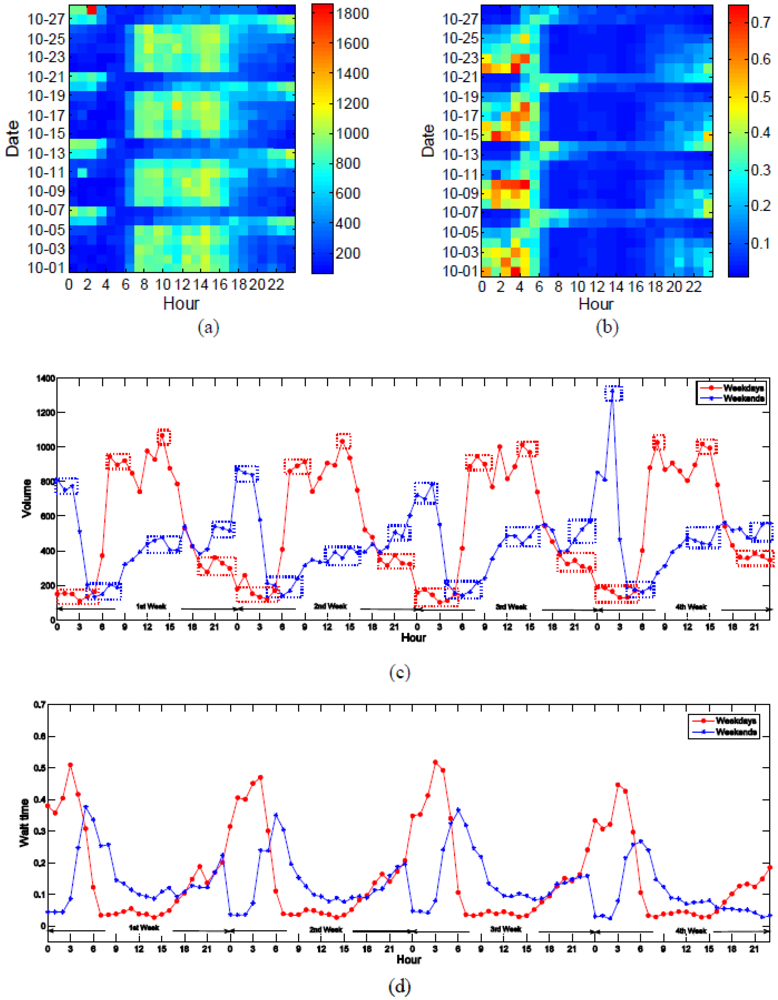


 ) or lognormal (
  ) distribution with high p-value passing the KS test [23] on either an hourly or a daily basis (Figure 8, Table 1 and Table 2). Importantly, the intensity of human activities during the rest periods (from 00:00 to 05:00 on weekdays and from 04:00 to 08:00 on the weekend) can be well approximated by the power law distributions, whereas all others agree well with the lognormal distributions. Moreover, here the power law distribution appears much more heterogeneous than the lognormal distribution, which can also be well observed in Figure 6.


 , where each item represents the coding symbol of the underlying spatial unit within which the current activity is taking place. To examine the patterns in the path string, the conventional method is based on Shannon [30] entropy which is a measurement of information within a system. Here, three typical methods are employed to quantify the information within a sequence of symbols. The first one is called the random entropy which is defined as
  , where N is the number of distinct symbols (spatial units) a path string (taxicab) has (visited). The random entropy treats every spatial unit as having the same visiting probability but ignores both the spatial (visiting frequency) and the temporal (visiting sequence) order of the visited regions. The order entropy is defined as
  , where pj is the probability of spatial unit j being visited. It considers the spatial order namely every region has different visiting probability, but it does not take into account the temporal order.

